HAL Id: hal-00267891
https://hal.archives-ouvertes.fr/hal-00267891
Submitted on 28 Mar 2008
Alain Ayong Le Kama, Katheline Schubert
To cite this version:
Alain Ayong Le Kama, Katheline Schubert. Growth, Environment and Uncertain Future Preferences. Environmental and Resource Economics, Springer, 2004, 28 (1), pp.31-53. �10.1023/B:EARE.0000023820.15522.a4�. �hal-00267891�
ALAIN AYONG LE KAMA
Université de Grenoble II, Commissariat général du Plan and EUREQua, Université de Paris I (adayong@univ-paris1.fr)
KATHELINE SCHUBERT
EUREQua, Université de Paris I (schubert@univ-paris1.fr)
Abstract. The attitude of future generations towards environmental assets may well be different from ours, and it is necessary to take into account this possibility explicitly in the current debate about environmental policy. The question we are addressing here is: should uncertainty about future preferences lead to a more conservative attitude towards environment? Previous literature shows that it is the case when society expects that on average future preferences will be more in favor of environment than ours, but this result relies heavily on the assumption of a separability between consumption and environmental quality in the utility function. We show that things are less simple when preferences are non-separable: the attitude of the society now depends not only on the expectation of the change in preferences but also on the characteristics of the economy (impatience, intertemporal flexibility, natural capacities of regeneration of the environment, relative preference for the environment), on its history (initial level of the environmental quality) and on the date at which preferences are expected to change (near or far future).
Keywords: Growth, Environment, Preferences, Uncertainty
1. Introduction
The attitude of future generations towards environmental assets may well be different from ours for many reasons, some of which are obvious and others unpredictable, since the formation of preferences involves complex and interlinked economic, social and moral determinants. It seems reasonable to think that we can infer future preferences from ours for the near future but not for the far distant one. However, environmental questions involve long-lasting phenomena, and current decisions will have long-lasting consequences. So it is necessary to take into account explicitly in the current debate about environmental policy the possibility of changes in preferences in the future. The question we are addressing here is: should uncertainty about future preferences lead to a more conservative attitude towards environment?1
Intuition could let us think that we should be more conservative now if we expect that future generations will value environment more than we do. Previous literature seems to confirm this intuition.
Beltratti, Chichilnisky and Heal (1993), Beltratti (1996) and Ayong Le Kama (2001) consider the evolution of an economy whose consump-tion is permitted by the depleconsump-tion of an exhaustible natural resource. Consumption is the sole source of welfare. A change in preferences may take place in the future at an unknown date and it modifies in an unknown way the level of utility associated to any level of con-sumption. The authors look at the consequences of this change on the optimal consumption path chosen by the central planner. They study the optimal preservation policy and show that uncertainty on future preferences leads to a more conservative use of the natural resource when the central planner expects that on average the preferences of future generations will be more in favor of environment than ours.
This paper studies more generally the optimal growth path of an economy facing a dilemma of consumption vs environmental quality. Consumption, which is a source of welfare, is permitted by the deterio-ration of environmental quality but this deteriodeterio-ration in turn diminishes welfare. Besides, consumption and environmental quality enter in a non-separable way into the utility function, and the relative weight of environmental quality is known with certainty only for the current generations and could be modified in the future at an unknown date and in an unknown direction. We then ask ourselves about the optimal management of environmental quality when facing this uncertainty. Beltratti, Chichilnisky and Heal (1998) also study the case in which the stock of exhaustible resource is a source of welfare and find the same intuitive result, but in a framework where the utility function is separable. This will prove to have important consequences because,
in the separable case, the marginal utility of consumption does not depend on the preference for the resource, and so is not affected by the change in preferences as it is in the non-separable case. Brasão and Cunha-e-Sâ (1998) extend the Beltratti, Chichilnisky and Heal (1998) framework to a capital-resource growth model, but retain the assumption of separable preferences. Their paper and this one taken together represent a complete extension of the previous results..
In order to be able to establish comparisons, we first study the case without any change in preferences (section 2). It will be our reference case. We then have a very simple model of growth with environment and the results are straightforward.
Section 3 explains the form taken by the change in preferences. Section 4 presents the case in which a change in preferences of an unknown direction occurs at a known date. We show that the optimal path satisfies the turnpike property. Before the change in preferences, the economy moves as long as possible near the optimal path when there is no change, and then the path of environmental quality is bended to reach its optimal target level at the time the change occurs. Under cer-tain circumstances, it can be optimal for the central planner to adopt a more conservative attitude from the beginning of the path to the date of the change in preferences, as it is the case in the Beltratti, Chichilnisky and Heal (1998) model. But whereas these circumstances depend only of the expectation of the change in preferences in Beltratti, Chichilnisky and Heal (1998), they are related here to the characteristics of the economy (impatience, intertemporal flexibility, natural capacities of re-generation of the environment, relative preference for the environment), to its history (initial level of the environmental quality) and also to the date at which preferences are expected to change (near or far future). Furthermore the optimal path, even if it is more conservative than the reference one, can only slightly be so for the near future, because of the turnpike property.
We study in section 5 the general case in which both the direction of the change and the time at which it will happen are unknown. We show that the turnpike property does not hold anymore. Depending on the initial level of environmental quality in relation to its stationary value and on the characteristics of the economy, the central planner will adjust consumption at the beginning of the optimal path upwards or downwards. He will then put the economy on a stationary equilibrium and wait there for the change in preferences to happen. In this case, it can therefore be optimal for the central planner to adopt a more conservative attitude at the beginning of the time horizon, as in the Beltratti, Chichilnisky and Heal (1993), Beltratti (1996) and Ayong Le Kama (2001) models. It may then also happen that consumption and
environmental quality decrease along the optimal path whereas they increase in the reference case.
Last, section 6 studies the special —and simpler— case of additively separable preferences and shows how the previous results are modified, and section 7 concludes.
2. The model without change in preferences
We study an economy in which environmental quality Q is depleted by consumption C, but regenerates itself at the constant rate ± > 0. Its evolution is then given by the following equation:
˙
Qt=±Qt− Ct: (1)
The central planner problem writes:
H(Q0) = maxR0∞e−½tu(Ct; Qt)dt s:t: ¯ ¯¯ ¯ ¯ ¯ ¯ ˙ Qt=±Qt− Ct Qt; Ct≥ 0 Q0 given ; ½ > 0
where ½ is the social discount rate.
We use a utility function u(C; Q) suitable with the existence of constant rate growth paths of consumption and environmental qual-ity. Smulders and Gradus (1996) show that a necessary condition for the existence of such paths is that preferences are characterized by a constant ratio of the value of environmental quality to the value of consumption, Q and C being valued at their marginal utility. This implies utility functions of the Cobb-Douglas form, such as:
u(C; Q) =
³
CQÁ´1−1¾
1 −¾1 ; (2)
where Á = QuCuQ
C > 0; which stands for the “relative preference for
environmental quality”, is constant in the course of time and ¾ is the intertemporal elasticity of substitution for consumption. We sup-pose that ¾ is strictly less than one2, which is sufficient to ensure that u (:) is concave and that the marginal utility of environmental quality decreases. Then the marginal utility of consumption increases when environmental quality deteriorates (uCQ < 0): utility exhibits a compensation effect, in the terminology of Michel and Rotillon (1996).
The current value Hamiltonian can be written as: H = u(C; Q) + ¸(±Q − C)
¸ being the shadow price of environmental quality. The first order necessary conditions are:
uC =¸ ˙¸ ¸ =½ − ± − uuQC ˙ Q Q =± − CQ (3)
and the transversality condition is: lim
t→∞e −½t¸
tQt= 0: (4)
By differentiating the first optimality condition and using the two others we easily find the growth rate of consumption g:
g = C˙ C =¾ · −½ + ± µ 1 +Á µ 1 − 1 ¾ ¶¶¸ +ÁC Q:
Let us define x = CQ; the previous equation allows us to write the following, in the stationary variablex:
˙ x
x = − [¾½ + (1 − ¾)(1 + Á)±] + (1 + Á)x: (5) The stationary solution of this equation is then given by:
x∗ = (1 − ¾)± + ¾½
1 +Á; (6)
which is strictly positive for ¾ < 1. The equation is unstable, so the economy will instantaneously switch to its stationary path at the beginning of the time horizon.
We then have an economy in which the CQ ratio is constant at the level x∗ andC and Q grow at the same rate g, with:
g = ± − x∗ =¾µ± − ½
1 +Á
: (7)
x∗ =± is the C
Q ratio that ensures the constancy of environmental
quality and consumption. If x∗ > ± i.e. if ½ > ±(1 + Á); the level
of consumption along the optimal path is relatively high vis-à-vis the level of environmental quality, and both decrease. This happens when the central planner is very impatient, or natural regeneration is low, or also the relative preference for environment is low. In the opposite case, consumption and environmental quality increase along the optimal path at the expense of a relatively small level of consumption.
Moreover, it is easy to show that the transversality condition is always satisfied and that the optimal value of the objective function is finite (see Appendix A (i)):
H(Q0) =
1
(1 +Á)x∗u(x∗Q0; Q0): (8)
3. The switch in preferences
A switch in preferences occurs once and for all and takes the form of a change in the relative preference for environment, the intertemporal elasticity of substitution¾ being given. We suppose that if this relative preference is initially Á, it can become:
à =
(
Á > Á with probability q ∈ [0; 1] Á < Á with probability 1 − q:
The corresponding utility functions are denoted by u(:) and u (:). Ã can be interpreted as the level of sensitivity to environment of the median consumer in an economy where a share q of consumers are likely to increase their preference for environment in the future while the others are likely to decrease it because of exogenous alterations of tastes. Or alternatively q can be seen as the probability of irreversible damage occurring to the environment in the future. This would enhance each agent’s preference for environment at the time the change takes place. 1−q is the probability of non-occurrence of this same damage, in which case concern for environment would decrease when uncertainty is resolved. We suppose Á ≥ 0; so that environmental quality cannot become a “bad” in the future.
For the central planner, the mathematical expectation of the new preference for environment of the representative consumer is:
E(Ã) = qÁ + (1 − q)Á: (9)
If E(Ã) = Á; the central planner expects that preferences will not change on average in the future. Following Beltratti (1996), Beltratti, Chichilnisky and Heal (1993) and (1998), this case is called symmetric uncertainty.
Moreover, it is important to notice that once the switch has oc-curred, the problem becomes identical with the previous one, the initial condition notwithstanding. So if the change in preferences appears at a given timeT > 0 the economy moves on a new growth path. It inherits
an environmental quality QT and, depending on the realization of Ã, it is then characterized by:
g = ¾³± − ½ 1+Á ´ x = (1 − ¾)± + ¾½ 1+Á or g = ¾µ± − 1+Á½ ¶ x = (1 − ¾)± +1+Á¾½
Thus if after time T the preference for environment increases the growth rate of the economy will be higher (g > g), and vice versa. This can be explained by the fact that a greater preference for environment translates into a relative decrease of consumption (level effect). This results in a greater accumulation of environmental quality and a greater growth rate (growth effect).
The value of the intertemporal welfare on the path followed after the change in preferences in each case is denoted byH(QT) orH(QT). 4. The model with an uncertain change in preferences at a
known date
We first study the case in which the central planner knows with cer-tainty that a change in the relative preference for environment will occur at a given time T , but does not know what change. This date can be broadly seen as the date at which the “present” generations are replaced by new generations, the “future” generations, about which we obviously lack informations because our life cycle does not overlap with theirs3.
4.1. The problem and its resolution: a turnpike property The central planner program writes (see Dasgupta and Heal (1974)):
maxR0T e−½tu(Ct; Qt)dt + e−½TE(H(QT)) ˙
Qt=±Qt− Ct
Qt; Ct≥ 0
Q0 given,
where the mathematical expectation of the remaining stock at the date of the change in preferences i.e. the expected bequest to the future generations is:
E(H(QT)) =qH(QT) + (1 − q)H(QT): (10)
The first order necessary conditions characterizing the evolution of the economy before the change in preferences are the same as when
preferences are unchanged. The dynamic equation in the stationary variable x is then still (5).
We must add to the first order conditions the following transversality condition:
¸T =E(H0(QT)) =qH0(QT) + (1 − q)H0(QT); (11)
which states that when the change in preferences occurs, the shadow price of environmental quality must be equal to the expected marginal value of the remaining stock.
We show (see Appendix A (ii)) that H0(QT) = uC(xQT; QT) and H0(QT) = u
C(xQT; QT), and besides we know from the first order
conditions that ¸T = uC(xTQT; QT); where xT is without ambiguity in notation the value of the ratio of consumption to environmental quality just before the change in preferences. So the expected marginal utility of consumption is the same immediately before the change in preferences and immediately afterwards:
uC(xTQT; QT) =quC(xQT; QT) + (1 − q)uC(xQT; QT):
This relationship allows us to obtain the value of the ratio of consump-tion to environmental quality just before the change occurs:
xT =F(QT); (12)
with:
F (Q) =hqx−¾1Q(Á−Á)(1−¾1) + (1 − q)x−¾1Q(Á−Á)(1−1¾)i−¾ > 0 ∀Q: (13) We will call equation (12) the No Expected Jump condition (NEJ).
The solution of the differential equation inx (5) is given by: 1 xt − 1 x∗ = µ 1 x0 − 1 x∗ ¶ e(1+Á)x∗t ∀t ∈ [0; T ] : (14)
This equation is unstable. So the only solution is to choose x0 as
close to x∗ as possible, then to stay as long as possible near the
refer-ence path, and finally to bend the path to hit the target xT: This is
reminiscent of the well-known turnpike property.
We easily show that the solution of the differential equation inQ is: Qt Q0 =e(±−x∗)t ·x 0 x∗ + µ 1 −x0 x∗ ¶ e(1+Á)x∗t¸ 1 1+Á ∀t ∈ [0; T] : (15)
Now, taking equations (14) and (15) at date T and eliminating x0
allows us to write the Euler condition:
with: Ψ(QT) =x∗ µ Qsup T QT ¶1+Á − 1 e(1+Á)x∗T − 1 ; (17)
where QsupT =Q0e±T is the maximal value that QT can reach4.
The Euler condition together with the Non Expected Jump condi-tion show us that the optimal level of environmental quality at the time the change occurs solves the following equation:
Ψ(QT) =F (QT): (18)
PROPOSITION 1. There is a unique solution to the problem with an uncertain change in preferences at a certain date.
Proof. We have Ψ(Q) > 0 ∀Q, lim
Q→0 Ψ(Q) = +∞; Ψ(Q sup
T ) = 0 and
Ψ0(Q) < 0.
So Ψ (:) is positive and strictly decreasing from +∞ to 0 on the interval [0; QsupT ]:
We also have, for any given q ∈ [0; 1] ; F(Q) > 0 ∀Q ∈ [0; QsupT ] and F(Qsup
T )> 0.
First, for q ∈ ]0; 1[ ; lim
Q→0F(Q) = 0; and F0 (Q) = (1 − ¾)F (Q) 1 ¾+1 Q : ³ (Á − Á)qx−¾1Q(Á−Á)(1−1¾)+ (Á − Á)(1 − q)x−1¾Q(Á−Á)(1−1¾)´;
with F0(Q)T 0 for Q SQ(q); unique, such that:e
e Q(q) = " (Á − Á)q (Á − Á)(1 − q) µx x ¶1 ¾# 1 (Á−Á)(1− 1¾ ) : (19)
So for q ∈ ]0; 1[ ; F (:) is positive, strictly increasing on the inter-val h0;Q(q)e h, and decreasing afterwards. As F(QsupT ) > 0, there is a unique intersection between the Ψ (:) and F (:) functions on the interval [0; QsupT ]:
Now for q = 1; F (:) is strictly increasing from 0 to F (QsupT ) > 0: So there is also a unique intersection between the Ψ (:) and F (:) functions on the interval [0; QsupT ]:
Last, for q = 0; F (:) is a concave function decreasing from infinity to zero. It can still easily be shown that there is a unique intersection
between the Ψ (:) and F (:) functions on the interval [0; QsupT ]: Equation (18) now writes: x∗ µ Qsup T QT ¶1+Á − 1 e(1+Á)x∗T − 1 =xQ (Á−Á)(1−¾) T ;
which is equivalent to: x∗
e(1+Á)x∗T
− 1
h
(QsupT )1+Á− Q1+ÁT i=xQ1+T Á+¾(Á−Á):
The LHS of this last equation is strictly decreasing from e(1+Á)x∗Tx∗ −1(QsupT )1+Á
to 0; while the RHS is strictly increasing from 0 to x (QsupT )1+Á+¾(Á−Á) on the interval [0; QsupT ].
Knowing the optimal value of QT, we can find the optimal paths of environmental quality and consumption before the change in prefer-ences:
− for environmental quality:
Qt=Q0egt ·x 0 x∗ + µ 1 − xx0∗ ¶ e(1+Á)x∗t¸ 1 1+Á ∀t ∈ [0; T ] (20) with x0 = x ∗ 1 + (x∗F (QT)−1− 1) e−(1+Á)x∗T (21) − for consumption: Ct=C0egt ·x 0 x∗ + µ 1 −xx0∗ ¶ e(1+Á)x∗t¸− Á 1+Á ∀t ∈ [0; T ] (22) withC0 =x0Q0.
Notice that it is possible to show, after a few manipulations, that u(Ct; Qt)
u(C0; Q0)
=e(1−1¾)(1+Á)gt ∀t ∈ [0; T ] :
the utility grows at a constant rate on the optimal path prior to the change in preferences, and this constant rate is identical to the growth rate reached when preferences do not change.
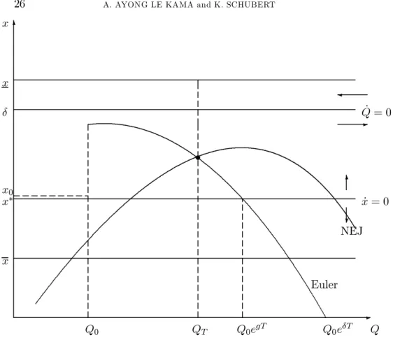
Figure 1 depicts the NEJ and Euler conditions in the (Q; x) plane and the phase diagram, and shows the paths followed by the economy before the change in preferences and afterwards, in the case where
the reference growth rate is positive and where the NEJ and Euler conditions cross abovex∗. When uncertainty about the direction of the
change resolves, consumption and the ratio of consumption to environ-mental quality jump upwards if there is a decrease in the preference for environment and downwards otherwise. In the first case, time T consumption and x ratio are high. This is due to the impatience of the economy associated with its low relative preference for environment, and finally leads to a decrease of consumption and environmental qual-ity in the course of time because of an insufficient accumulation of environmental quality. It is the opposite in the second case.
<figure 1 here> 4.2. A comparison with the reference path
We now come to the point that motivated this study: is the society more or less conservative in the presence of an uncertainty about future preferences?
4.2.1. The definition of a more conservative society
Let’s first define more precisely what we mean by conservative. DEFINITION. We will say that the society is more conservative in the presence of an uncertainty if the path of the ratio of consumption to environmental quality is under its reference path (its path without uncertainty), from the origin to the date at which preferences change. The society will be all the more conservative as the distance between the two trajectories will be great.
First of all, equation (21) shows that x0 < x∗ iff x∗ > F (QT)
i.e., with equation (12), iff xT < x∗. Moreover, the motion of x is
monotonous so, if the path of x is under the reference path at the origin and also when preferences change, it will be under it in between. Our definition of a more conservative society is thus meaningful.
Furthermore, we show in Appendix A (ii) that the marginal value of the bequest is, at the date of the change in preferences,
E¡H0(QT)¢=Q−¾1 T " q x1 ¾Q Á(1−1¾) T +1 − q x1 ¾ Q Á(1−1 ¾) T # ;
besides, the marginal utility of consumption is at the same date, on the reference path, uC(x∗QT; QT) = x∗ − 1 ¾ Q− 1 ¾+Á(1−1¾) T ;
so E(H0(QT)) uC(x∗QT; QT) = µ x∗ F(QT) ¶1 ¾ :
The central planner will thus be more conservative if the expected marginal value of the bequest is higher than the reference marginal utility of consumption at the time the change occurs.
Equation (21) also shows that if the date T at which preferences change is far from now x0 is very close to x∗ (turnpike property) so,
as the initial environmental quality Q0 is the same with and without
the change in preferences, the initial consumption is very close to its reference value. So, even if the central planner is more conservative, he will not be much more conservative at the beginning of the trajectory if the change is to happen in the far future.
We can verify that if the optimal path is more conservative than the reference one, society enjoys a higher environmental quality at the time the change in preferences occurs: using equation (18) it is easy to show, after some manipulations, that x∗> F (QT) ⇔ QT > Q0egT.
We can also show (see Appendix B) that if the optimal path is more conservative than the reference one consumption is smaller on the optimal path than on the reference one when the change in preferences occurs: CT < x∗Q0egT; that is not obvious because CT =xTQT; with
xT < x∗ but QT > Q0egT:
4.2.2. The conditions for a more conservative society
Now, if x∗ = F(QT) i.e. if QT = Q0egT; the optimal path is exactly
identical to the reference one before the change in preferences. Equation (18) shows that:
QT T Q0egT ⇔ Ψ(Q0egT)T F(Q0egT) ⇔ x∗ T F(Q0egT):
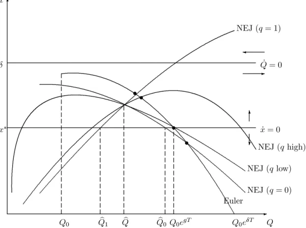
Figure 2 draws the F (Q) function for different values of the prob-ability q; in order to find the (qualitative) conditions for which the optimal path is more or less conservative than the reference one.
<figure 2 about here>
There exists a level of environmental quality denoted Q such thatb F(Q) is the same for every possible value of the probability q; and it isb
easy to find this level:
b Q =µxx¶ 1 (Á−Á)(1−¾) (23) We have:
F (Q) =b à xÁ−Á xÁ−Á ! 1 Á−Á
and we show in Appendix C thatF (Q) > xb ∗:
Besides, using equations (23) and (19), we can find the probability q for which the maximum of the F(Q) function is Q :b
b Q =Q(q) ⇐⇒e µx x ¶ 1 (Á−Á)(1−¾) = " (Á − Á)q (Á − Á)(1 − q) µx x ¶1 ¾# 1 (Á−Á)(1− 1¾ ) ⇐⇒ qÁ + (1 − q)Á = Á ⇐⇒ E(Ã) = Á ⇐⇒ q = Á − Á Á − Á and for qS Á−Á Á−Á we have Q(q)e SQ.b
Finally, when the central planner knows with certainty that the relative preference for environment will increase (q = 1), the F(Q) function is strictly increasing from zero to infinity, and we define Qb1
by:
F (Qb1)¯¯¯
q=1=x ∗
Symmetrically, when the central planner knows with certainty that the relative preference for environment will decrease (q = 0), the F(Q) function is strictly decreasing from infinity to zero, and we define Qb0
by:
F (Qb0)¯¯¯
q=0=x ∗
We easily show that:
b Q0= ¡x x∗ ¢ 1 (Á−Á)(1−¾) b Q1= ³x∗ x ´ 1 (Á−Á)(1−¾) b Q1<Q <b Qb0 (24)
We then see that ifQ0egT is low and, more precisely, ifQ0egT <Qb1;
the central planner will be all the more conservative than the probabil-ity of the change is high. We will call this case a case of “bad reference path”. A society experiencing a bad reference path has poor environ-mental conditions (the initial environenviron-mental qualityQ0is low and so is
the natural regeneration rate ±), is very impatient (the social discount rate ½ is high), and does not care very much about environment (Á is low); furthermore, it expects that the change in preferences will happen in the near future (T is small) and so uncertainty is pressing. Such a society will have incentives to be more conservative if the probability of a positive change of the relative preference for environment is very high. In this case, we will say that the central planner adopts a precautionary behavior.
If, on the contrary,Q0egT >Qb0; which is the case depicted in Figure
2 for different probabilities of a positive change in the relative prefer-ence for environment q, then the central planner will be all the more conservative than the probability of a positive change is low. This case is a case of “good reference path”. A society on a good reference path has fair environmental conditions, is patient and cares about environment. The central planner will have incentives to be more conservative only if he expects a decrease in the relative preference for environment in the far future. In this case, we will say that he adopts an insurance behavior against a worsening of environmental conditions.
Finally, if Qb1 ≤ Q0egT ≤Qb0; the society will never be more
conser-vative, whatever the probability q of a positive change in the relative preference for environment.
5. The problem with an uncertain change in preferences at an uncertain date
We now suppose that when he decides of the path followed by the economy the central planner knows neither what the future generations preferences will be nor the date at which a change in preferences could occur. The two types of uncertainty are independent. The full problem is then: maxEhR0T e−½tu(Ct; Qt)dt + e−½TH(QT)i ˙ Qt=±Qt− Ct Qt; Ct≥ 0 Q0 given,
where the dateT at which the change in preferences occur is a random variable, with marginal density !tand Ωt=Rt∞!¿d¿. The maximand of this problem can be reformulated as:
max Z ∞ 0 !T "Z T 0 e −½tu(Ct; Qt)dt + e−½TE(H(QT)) # ;
or, after integrating by part (see Dasgupta and Heal (1974)): max Z ∞ 0 e −½t[Ωtu(Ct; Qt) +!tE(H(Qt))]dt: 5.1. Analytical resolution The current value Hamiltonian is:
H = Ωu(C; Q) + !E(H(Q)) + ¸(±Q − C); and the first order conditions are:
(
ΩuC =¸
˙ ¸
¸ =½ − ± − ÁCQ−Ωu!CE(H0(Q)):
Differentiating the first optimality condition and using QQ˙ =± − CQ we obtain: ˙ C C =¾ µ 1 +Á µ 1 −¾1 ¶¶ ± − ¾½ + ÁCQ −¾Ω! ·1 −E(H 0(Q)) uC ¸ ; (25) where !t
Ωt is the probability for the change to occur at timet given that
it has not previously occurred.
We have seen (Appendix A (ii) and previous section) that the ratio of the marginal value of the bequest to the reference marginal utility of consumption is, at a given date t; uE(H0(Q))
C(xQ;Q) =
³ x
F (Q)
´1
¾ with F(Q)
previously defined (equation (13)). So we obtain the following equation for the growth rate of consumption before the change in preferences:
˙ C C =¾ ·µ 1 +Á µ 1 −¾1 ¶¶ ± − ½ −Ω!¸+Áx + ¾! Ω µ x F(Q) ¶1 ¾ : (26) Assumption 1: The marginal density !t of the random future date t at which the change in preferences occurs is a Poisson process with constant parameter¹: Thus we have !t
Ωt =¹ ∀t:
Under this assumption and using equation (26), the differential equa-tions in x and Q characterizing the evolution of the economy and the environment before the change in preferences are:
˙ x x = (1 +Á)(x − x∗) +¾¹ µ³ x F (Q) ´1 ¾ − 1 ¶ ˙ Q Q =± − x (27)
5.1.1. Existence of a stationary equilibrium
A stationary equilibrium (xs; Qs) of this system is characterized by
˙ x x =
˙ Q
Q = 0. This leads toxs =± and Qs is a solution of the following
equation: F(Qs) =± · 1 −1 +¾¹Ág ¸−¾ : (28)
We have to make sure that the term into brackets in the RHS of this equation is positive5. It needs¹ > (1 + Á)± − ½: When this condition is
fulfilled, for q ∈ ]0; 1[ if F(Q(q)) < ±e h1 −1+Á¾¹ gi−¾ (with Q(q) definede in equation (19)), equation (28) does not admit any solution, and for the opposite case there exist two solutions. For q = 0 or 1 there is a unique stationary equilibrium.
5.1.2. Stability of stationary equilibria
When we linearize the dynamic system (27) around a steady state — when it exists— we get the following Jacobian matrix:
A =
Ã
½ + ¹ −¹h1 −1+Á¾¹ gi1+¾F0(Qs)
−Qs 0
!
withtrA > 0 and det A of the opposite sign as F0(Qs). Among the two possible values of Qswe must then choose the smallest one in order to have F0(Qs)> 0 and consequently a saddle-path.
Notice that for q = 0; given that F0(Q) < 0; ∀Q even if there exists
a stationary equilibrium, this equilibrium is unstable.
PROPOSITION 2. For any given q ∈ ]0; 1] ; if ¹ > (1 + Á)± − ½ and F(Q(q)) ≥ ±e h1 −1+Á¾¹ gi−¾ there exists a stable path solution of the problem with an uncertain change in preferences at an uncertain date whose stationary equilibrium is a saddle-point characterized by xs=±, F(Qs) =±
h
1 −1+Á¾¹ gi−¾ and F0(Qs)> 0:
When this solution exists, note that we have dQs d¹ = − 1 F0(Qs) ±(1 + Á) ¹2 g · 1 −1 +¾¹Ág ¸−¾−1 ;
which has the opposite sign as g: Thus when the parameters are such that consumption and environmental quality grow in the reference case, the stationary level of environmental quality Qs is all the smaller as the flow probability of occurrence of the change in preferences is high.
In order to finish to characterize the path prior to the change in preferences, we have to find x0 as a function of Q0 and the shape of
the convergence to the stationary state. The negative root of matrix A is:
h = 12 ½ + ¹ − s (½ + ¹)2+ 4¹ · 1 − 1 +¾¹Ág ¸1+¾ QsF0(Qs) :
One can find the initial condition necessary and sufficient for the econ-omy to converge to the saddle-point along the linearized path:
x0 =± + h µ 1 −QQ0 s ¶ : (29)
5.2. A comparison with the reference path
The society will be more conservative in the uncertain case than in the reference case if the path of the ratio of consumption to environmen-tal quality is under its reference path i.e. if x0 < x∗ and xs < x∗6:
This latter condition is satisfied if the growth rate of the economy in the reference case g is negative. The former can be written, due to equation (29), as ± + h³1 −Q0 Qs ´ < x∗ ⇔ Q0 <¡1 + g h ¢ Qs: The initial
environmental quality must then be rather low. Furthermore, the ratio of consumption to environmental quality decreases along the optimal path (but at a smaller rate than in the reference case) iff x0 > xs=±;
which needs Q0> Qs; and increases otherwise.
Besides, given the shape of the F (Q) function, we see easily that, for a given set of parameters such that consumption and environmental quality decrease in the reference case (g < 0) and for ¹ given, we have ±h1 −1+Á¾¹ gi−¾ < ± < x∗ < F (Q) ≤ Fb ³Q(q)e ´∀q ∈ ]0; 1] ; Q being theb environmental quality for which F (Q) is the same for every possible value of the probability q and Q(q) being the maximum of the F(Q)e function for a given probability q ∈ ]0; 1]. So in this case there exists a unique solution to equation (28) on the increasing branch of the F(Q) function, and this solution, the stationary level of environmental quality Qs; is all the higher since the probability of a positive change in
prefer-ences (q) is high. Everything takes place as if the central planner of an economy experiencing a poor reference growth would, while waiting for the change in preferences to happen, put this economy on a stationary path characterized by an environmental quality all the higher as the probability of a positive change is high.
Things are similar when the parameters are such that g > 0 and ±h1 −1+Á¾¹ gi−¾ < F(Q): Qb s is all the higher sinceq is high.
But things are different when g > 0 and ±h1 − 1+Á¾¹ gi−¾ > F (Q):b We can find the probability q; denoted by q; for which F (e Q(e q)) =e ±h1 −1+Á¾¹ gi−¾: If E(Ã) < Á; q is the highest probability for which ae
solution to equation (28) exists, and the nearer q is to q the higher ise
Qs. If E(Ã) > Á;q is the smallest probability for which a solution toe
equation (28) exists, and the higher isq with respects toq the smalleste
isQs: So in the case of an economy enjoying a great reference growth (g high enough to imply±h1 − 1+Á¾¹ gi−¾ > F(Q)) and of a central plannerb expecting that on average the future preference for environment will be greater than the present one (E(Ã) > Á), this central planner will, while waiting for the change in preferences to happen, put the economy on a stationary path characterized by an environmental quality all the poorer as the probability of a positive change is high.
Figure 3 shows the phase diagram in the (Q; x) plane and the path followed by the economy when the growth rate in the reference case is positive (thus the society is less conservative) and the initial envi-ronmental qualityQ0 is greater than the stationary one Qs. The latter
depends only on parameters (social discount rate, natural regeneration rate, preference parameters) and on the probabilities q and ¹. As in the reference case consumption is growing, we have seen that Qs is all the smaller as ¹ is high.
In this case where we have an initial stock greater than the sta-tionary one, even though it is optimal for the chosen parameters to let consumption and environmental quality grow in the reference case at the expense of a small initial consumption, it is optimal in the case with uncertainty to consume a great deal at the beginning of the path and to let consumption and environmental quality decrease towards their stationary value.
<figure 3 here>
6. The special case of separable preferences
In the case of a unit intertemporal elasticity of substitution for con-sumption, the initial utility function is additively separable and is stated simply asu(C; Q) = ln C +Á ln Q. We study this case in order to stress the importance of the non-separability assumption, which allows us to obtain qualitatively different results.
6.1. The model without change in preferences
The problem is solved as in the general case. Equations (6) and (7)
become: (
x∗ = ½ 1+Á
g = ± − x∗ =± − ½ 1+Á:
6.2. The case of an uncertain change in preferences at a certain date
The path subsequent to the change in preferences is easily deduced from the general case.
As for the path prior to the change in preferences, we now have: F(Q) =µxq +1 − q
x
¶−1
=½h1 +Áq + Á(1 − q)i−1 = ½ 1 +E(Ã) with E(Ã) given by equation (9). F (Q) does not depend on Q any more; so equation (18) becomes
x∗ µ Qsup T QT ¶1+Á − 1 e(1+Á)x∗T − 1 = ½ 1 +E(Ã); (30)
and allows us to obtain QT explicitly: QT =Q0egT µ 1 +E(Ã) 1 +Á + (E(Ã) − Á)e−½T ¶ 1 1+Á ; (31)
whereQ0egT is the level of environmental quality at timeT when there
is no change in preferences. A case of symmetric uncertainty in the sense of Beltratti (1996), Beltratti, Chichilnisky and Heal (1993) and (1998) can appear here, corresponding to E(Ã) = Áq + Á(1 − q) = Á. Then QT =Q0egT and the economy follows the reference path before
the change in preferences. We obviously have QT > Q0egT iff E(Ã) >
Á and QT < Q0egT otherwise: the central planner who expects on
average a positive change in the relative preference for environment will choose to have a more conservative attitude towards environment, and the planner who expects on average a decrease in the preference for environment will be less conservative.
The transversality condition (equation (12)) now writes xT = F =
½
1+E(Ã) and we have xT S x∗ ⇔ E(Ã) T Á:
Lastly, we can show thatx0 is explicitly given by:
x0 = x
∗
1 +¡xF∗ − 1¢e−(1+Á)x∗T =
½
and we see that xT < x0 < x∗ ⇔ E(Ã) > Á: The turnpike property
does not hold anymore: if the central planner expects that on average the preference for environment will be greater in the future, the ratio of consumption to environmental quality is always smaller than in the reference case before the change in preferences, that is to say that the society is always more conservative.
6.3. The case of an uncertain change in preferences at an uncertain date
The system (27) is now written as:
˙ x x = −(½ + ¹) + (1 + Á + ¹1+E(Ã)½ )x ˙ Q Q =± − x:
x immediately takes its stationary value, given by:
ee
x = ½ + ¹
1 +Á + ¹1+E(Ã)½ =
½ 1 +½Á+¹E(Ã)½+¹
that is, everything takes place as if the preference for environment would become ½Á+¹E(Ã)½+¹ ; a weighted average of the actual (Á) and the expected (E(Ã)) relative preferences for the environment, the weights being respectively the impatience of the society (½) and its appreciation of risk (¹). We easily show that:
ee
x S x∗ ⇐⇒ E(Ã) T Á:
Consumption and environmental quality evolve at a rate± −x untilee uncertainty is resolved. If x < xee ∗ this rate is greater than in the case
without change in preferences, and the initial consumption smaller. The optimal behavior towards environment is more conservative —this is rather intuitive— since the central planner expects an increase in the relative preference for environment.
7. Concluding remarks
The question we have addressed here is: should uncertainty about future preferences lead to a more conservative attitude towards en-vironment? Beltratti (1996), Beltratti, Chichilnisky and Heal (1993) and (1998), and Ayong Le Kama (2001) answer that if we believe that future generations will have on average a stronger preference for
environment than ours, then our optimal attitude is to be more con-servative from now. We have shown that this result suffers from a lack of generality and strongly depends on the assumption of a separability of consumption and environmental quality in the utility function. But the issue of whether such a utility function is separable or not is very hard to ascertain, and it seems useful to study the implications of a non-separability.
In the case where the central planner knows with certainty when the change in preferences will occur, we have shown that before the change actually happens he never has strong incentives to be immediately more conservative, relative to the situation without change in preferences. The optimal behavior is to stay close to the reference path now and in the near future, and to become notably more conservative near the date of the change in preferences under certain conditions related to the characteristics of the economy, its history, and the value of the probability of a positive change in preferences.
In the case where there is besides uncertainty about the date at which the change in preferences will occur, it can be optimal for the central planner to adopt a conservative attitude as in the Beltratti, Chichilnisky and Heal (1998) model, even if the motives of conservation are different. This happens when the growth rate of the economy is neg-ative in the reference case (high social discount rate, small regeneration rate and/or small relative preference for environment) and when the initial environmental quality is low. But, depending on the characteris-tics of the economy, it may also occur that the central planner, knowing that a change in preferences will take place, but knowing neither when nor in which direction, will lead the economy to consume very highly before the change occurs, as an insurance against latter deprivations.
We probably have good reasons to suspect that people will care more about environment in the future than we do now, for example because environmental problems will become more pressing. We show that under our assumptions it is not in itself a sufficient motive for modifying notably our present behavior. If the decision maker ignores the time at which the change in preferences will occur, two kinds of behaviors are possible. Firstly, if the economy has poor prospects of growth and a bad environmental quality, it will rather adopt a pre-cautionary behavior and be more conservative. But if on the contrary the growth path without change in preferences is favourable and the environmental quality fair, the society will rather adopt a behavior of insurance against later deprivations, consisting in consuming a great deal now at the expense of environmental quality. This could explain for example the attitude of many developed countries in the face of the global warming prospect.
Appendix
A. The value of the intertemporal welfare
(i) In the problem without change in preferences we know that con-sumption and environmental quality grow at the same rate± − x∗; and
that their ratio is constant at the level x∗: So we can write: H(Q0) = u(C0; Q0) Z ∞ 0 e −½te(±−x∗)(1+Á)(1−1 ¾)tdt = u(C0; Q0) Z ∞ 0 e −(¾½+(1−¾)±(1+Á))tdt = u(x∗Q0; Q0) 1 (1 +Á)x∗;
which is finite for any finite value of Q0, given thatx∗> 0:
(ii) Now, given the value of H(Q0); we deduce the marginal
intertem-poral welfare: H0(Q 0) = 1 (1 +Á)x∗[x ∗u C(C0; Q0) +uQ(C0; Q0)] = 1 (1 +Á)x∗[x ∗u C(C0; Q0) +Áx∗uC(C0; Q0)] = uC(x∗Q0; Q0):
Thus we also have the marginal values of the bequest in the problem in which preferences change:
(
H0(Q
T) =uC(xQT; QT)
H0(QT) =u
C(xQT; QT);
and the expected marginal value of the bequest: E¡H0(Q T)¢ = quC(xQT; QT) + (1 − q)uC(xQT; QT) = Q− 1 ¾ T " q x1 ¾Q Á(1−1 ¾) T +1 − q x1 ¾ Q Á(1−¾1) T # : B. Consumption when the central planner is more conservative, in the case of an uncertain change in preferences at a certain date
When the optimal path is more conservative than the reference one the value of consumption on the optimal path is not obviously smaller than
on the reference one when the change in preferences occurs because, CT =xTQT; with xT < x∗ but QT > Q0egT:
Equation (22) allows to write: CT x∗Q0egT = x0 x∗ ·x 0 x∗ + µ 1 − xx0∗ ¶ e(1+Á)x∗T¸− Á 1+Á and CT x∗Q0egT < 1 ⇐⇒ x0 x∗ < ·x 0 x∗ + µ 1 −xx0∗ ¶ e(1+Á)x∗T¸ Á 1+Á ⇐⇒ µx 0 x∗ ¶1+Á Á < x0 x∗ + µ 1 −xx0∗ ¶ e(1+Á)x∗T
which is always verified if the society is more conservative, because in this case x0
x∗ < 1:
C. The position of the F (Q) function F(Q) > xb ∗ ⇐⇒ x∗ Á−Á< xÁ−ÁxÁ−Á ⇐⇒ µx∗ x ¶Á−Á <µxx∗¶Á−Á ⇐⇒ (Á − Á) ln µx∗ x ¶ < (Á − Á) lnµxx∗¶ which happens to be true if x∗; x and x are not too different:
x x∗ = 1 +¾½x∗ µ 1 1+Á−1+Á1 ¶ = 1 +¾½x∗ Á−Á (1+Á)(1+Á) x x∗ = 1 +¾½x∗ ³ 1 1+Á− 1 1+Á ´ = 1 +¾½x∗ Á−Á (1+Á)(1+Á) =⇒ lnxx∗ ' ¾½x∗ Á−Á (1+Á)(1+Á) lnxx∗ ' ¾½x∗ Á−Á (1+Á)(1+Á) thus (Á−Á) ln µx x∗ ¶ +(Á−Á) ln µ x x∗ ¶ ' ¾½x∗ (Á − Á)(Á − Á)1 +Á " 1 1 +Á − 1 1 +Á # > 0: Acknowledgements
We are grateful for the comments of the participants of the Work-shop on Environmental Economics of EUREQua. We also thank An-toine d’Autume, David Ulph and especially Sjak Smulders for helpful discussions. Any remaining shortcomings are our responsibility.
Notes
1Heal and Kriström stress the relevance of this question in the case of climate
change.
2In section 6, we study the special case of additively separable utility functions
(¾ = 1).
3These future generations could be let’s say the generations beginning with the
children of our grandchildren, who will be grown up in fifty years or so.
4
Before the change in preferences occurs, environmental qualityQ grows at the rate (± − x) with x ≥ 0: So for Q0 given,QT ≤ QsupT :
5
This is always the case wheng ≤ 0:
6
It may happen that the society is actually more conservative withx0< x∗and
xs > x∗; if uncertainty resolves at a early date T such that xT < x∗; we do not
however describe this situation as more conservative, because the central planner does not intend to be so.
References
Ayong Le Kama, A. (2001), ‘Preservation and Uncertain Future Preferences’. Economic Theory, 8(3):745—752.
Beltratti, A. (1996), Models of Economic Growth with Environmental Assets. Kluwer Academic Publishers, Fondazione ENI Enrico Mattei series on Economics, Energy and Environment.
Beltratti, A. G., G. Chichilnisky and G. M. Heal (1993), ‘Preservation, Uncertain Future Preferences and Irreversibility’. Nota di Lavoro 59.93, Fondazione ENI Enrico Mattei, Milan.
Beltratti, A. G., G. Chichilnisky and G. M. Heal (1998), ‘Uncertain Future Preferences and Conservation’. In G. Chichilnisky and G. M. Heal, editors, Sus-tainability: Dynamics and Uncertainty. Kluwer Academic Publishers, Fondazione ENI Enrico Mattei series on Economics, Energy and Environment.
Brasão, A. and M. Cunha-e-Sâ (1998), ‘Optimal Growth, Uncertain Future Prefer-ences and Preservation’. Universidade Nova de Lisboa, Faculdade de Economia. Paper presented at the First World Congress, EARE/EAERE, Venice, June 25—27.
Dasgupta, P. S. and G. M. Heal (1974), ‘The Optimal Depletion of Exhaustible Resources. Review of Economic Studies, Symposium Issue, 3—28.
Heal G. and B. Kriström (2002), ‘Uncertainty and Climate Change’. Environmental and Resource Economics, 22(1—2):3—39.
Michel, P. and G. Rotillon (1996), ‘Desutility of Pollution and Endogenous Growth’. Environmental and Resource Economics, 6:279—300.
Smulders, S. and R. Gradus (1996), ‘Pollution Abatement and Long-term Growth’. European Journal of Political Economy, 12:505—532.
-6 • Q Q0 QT Q0egT Q0e±T x∗ ± x x x0 x ˙ x = 0 ˙ Q = 0 Euler NEJ ? 6 -¾
Figure 1. Change in preferences at a certain date, non-separable preferences, case g > g > 0, g < 0, QT < Q0egT
-6 • • • • NEJ (q = 1) NEJ (q high) NEJ (q low) NEJ (q = 0) Euler Q Q0 Qb1 Qb Qb0 Q0egT Q0e±T x∗ ± x ˙ x = 0 ˙ Q = 0 ? 6 -¾
Figure 2. Change in preferences at a certain date, non-separable preferences, caseg > 0, Q0egT >Qb0
-6 ? 6 -¾ x∗ ± x x x0 x Q Qs Q0 ˙ x = 0 ˙ Q = 0
Figure 3. Change in preferences at an uncertain date, non-separable preferences, case Qs< Q0,g > g > 0, g < 0