Dynamic marketing policies : constructing Markov states for reinforcement learning

(1)

Dynamic Marketing Policies: Constructing Markov States

for Reinforcement Learning

By Yuting Zhu

B.A. in Economics, Renmin University of China (2015) B.S. in Mathematics, Renmin University of China (2015)

M.A. in Economics, University of Rochester (2017)

SUBMITTED TO THE SLOAN SCHOOL OF MANAGEMENT IN PARTIAL FULFILLMENT OF THE REQUIREMENTS FOR THE DEGREE OF

MASTER OF SCIENCE IN MANAGEMENT RESEARCH at the

MASSACHUSETTS INSTITUTE OF TECHNOLOGY MAY 2020

Signature of Author:__________________________________________________________ Department of Management

MAY 04, 2020

Certified by: ________________________________________________________________ Juanjuan Zhang John D.C. Little Professor of Marketing Thesis Supervisor

Accepted by: _______________________________________________________________ Catherine Tucker Sloan Distinguished Professor of Management

Professor, Marketing Faculty Chair, MIT Sloan PhD Program

(2)

(3)

Dynamic Marketing Policies: Constructing Markov States for

Reinforcement Learning

by

Yuting Zhu

Submitted to the THE SLOAN SCHOOL OF MANAGEMENT on MAY 04, 2020, in partial fulfillment of the

requirements for the degree of

MASTER OF SCIENCE IN MANAGEMENT RESEARCH

Abstract

Many firms want to target their customers with a sequence of marketing actions, rather than just a single action. we interpret sequential targeting problems as a Markov Decision Process (MDP), which can be solved using a range of Reinforcement Learning (RL) algorithms. MDPs require the construction of Markov state spaces. These state spaces summarize the current information about each customer in each time period, so that movements over time between Markov states describe customers’ dynamic paths. The Markov property requires that the states are “memoryless,” so that future outcomes depend only upon the current state, not upon earlier states. Even small breaches of this property can dramatically undermine the performance of RL algorithms. Yet most methods for designing states, such as grouping customers by the recency, frequency and monetary value of past transactions (RFM), are not guaranteed to yield Markov states.

We propose a method for constructing Markov states from historical transaction data by adapting a method that has been proposed in the computer science literature. Rather than designing states in transaction space, we construct predictions over how customers will respond to a firm’s marketing actions. We then design states using these predictions, grouping customers together if their predicted behavior is similar. To make this approach computationally tractable, we adapt the method to exploit a common feature of transaction data (sparsity). As a result, a problem that faces com-putational challenges in many settings, becomes more feasible in a marketing setting. The method is straightforward to implement, and the resulting states can be used in standard RL algorithms. We evaluate the method using a novel validation approach. The findings confirm that the constructed states satisfy the Markov property, and are robust to the introduction of non-Markov distortions in the data.1

Thesis Supervisor: Juanjuan Zhang

Title: John D.C. Little Professor of Marketing

(4)

(5)

List of Figures

A-1 Histogram of Customer Outcomes in the Six Experiments . . . 55 A-2 System Dynamic Matrix . . . 56 A-3 Error Rates Under the Current Policy Using the True Probabilities . 56 A-4 Error Rates Under the Optimal Policy Using the True Probabilities . 57 A-5 Proportion of States that Satisfy the Markov Property . . . 57

(8)

(9)

List of Tables

B.1 Sample Sizes in Six Experiments . . . 60 B.2 Effect of Estimated Probabilities . . . 60 B.3 Model-Free Evidence: Error Rates of Length-Two Profits . . . 60

(10)

(11)

Chapter 1 Introduction

Standard targeting models are myopic. They treat marketing actions as single period decisions with single period outcomes. However, in practice, firms can often imple-ment a sequence of marketing actions in order to affect current and future outcomes. For example, instead of just deciding which customers to call (and which not to call), it may be optimal to call, then email, then mail to one customer, while for another customer it is optimal to call twice and then email.

A sequential targeting problem can be interpreted as a Markov Decision Process (MDP), which can be solved using a range of Reinforcement Learning methods. We will formally define MDPs in Section 3, but we can illustrate the concept using a baseball example. The objective of the batting team is to score as many runs as possible in each inning. At each point in time, the situation can be summarized using a finite set of possible states. For example, suppose there is a runner on first base, the other bases are empty, and there is one out in the inning. We will label this as State 1. A key feature of an MDP is that there is a decision to be made. In our example, we will focus on the runner’s decision to attempt to steal second base (for simplicity we will ignore the actions and outcomes for the batter). The runner has two action options (his “action space”): he can attempt to steal or not. If he steals and succeeds, the new state of the game will be: a runner on second base, other bases are empty, and there is one out in the inning (we will denote this as State 2). In contrast, if the runner steals and fails, the state of the game will change to: all of the bases are

(12)

empty and there are two outs (denote this as State 3). Thus, the choice of action by the runner affects the transitions to future states.

The transitions to future states in turn affect the expected number of runs the team will score in that inning (the “expected rewards”). A simple empirical average from past Major League Baseball games reveals that on average a team scores 0.5088 runs in State 1, 0.6675 runs in State 2 and 0.0986 runs in State 3. Using these expected rewards, we can calculate the values associated with each action in State 1 (the “state-action pairs”): if the runner does not attempt to steal we remain in State 1 and expect to score 0.5088 runs. If the runner steals, the expected rewards from the State1-Steal (state-action) pair is: 0.6675 * 𝛽 + 0.0986 * (1 − 𝛽), where 𝛽 is the probability of success. By comparing the values of the two state-actions pairs (State 1-Steal and State 1-Not Steal), the runner can choose the optimal action in State 1. In this case, the runner should steal as long as the probability of success exceeds 0.7201. This probability might also be estimated by observing past outcomes (ideally past outcomes for that runner and that pitcher).

Notice that the value associated with attempting a steal incorporates the long-term impact of the current action. This also allows the choice of the current action to incorporate the impact of future actions. For example, if the runner is particularly good at stealing bases, and so is also likely to successfully steal from second base to third base, this will increase the expected number of runs the team will score in State 2. The expected rewards for State1-Steal should (and would) incorporate this adjustment. The states we have described are just three of many possible states in baseball. Players can learn the optimal action in the other states using a similar process.

It is helpful to list the four steps in the process:

1. Design states that summarize the situation in each time period. These time periods typically match the timing in which a decision-maker (a firm) needs to choose actions (whether or not to call a customer).

(13)

rewards and transition probabilities from the current state to any possible states. In our baseball example, the transition probability for the State 1- Steal pair, is 𝛽 to State 2 and (1 − 𝛽) to State 3.

3. Estimate the value of each state-action pair for a given policy (“Policy Eval-uation”). This is typically the expected value of current rewards (if any) to-gether with the expected value of the rewards in future states. For example, in our baseball example, the value of the State1-Steal pair is calculated as 0.6675 * 𝛽 + 0.0986 * (1 − 𝛽).

4. Improve the policy by choosing the action in each state that has the highest value (“Policy Improvement”). In State 1 the runner only steals second base if 0.5088 < 0.6675 * 𝛽 + 0.0986 * (1 − 𝛽).

Standard Reinforcement Learning (RL) algorithms mimic this logic; a typical RL algorithm uses the same four steps. Steps 1 and 2 can be thought of as preliminary steps. Once the states are designed and the transition probabilities estimated, we do not re-visit Steps 1 and 2. However, because the value of each state-action pair depends upon the actions in future states, Steps 3 and 4 (Policy Evaluation and Policy Improvement) are solved iteratively. We value the current state-action pairs using an initial policy (choice of actions in each state), we then use the values of each state-action pair to improve the policy. We can then re-value the state-action pairs under this improved policy, and then further improve the policy. This is the standard iterative approach for solving RL problems, and there are theoretical guarantees on its performance (we discuss this iterative approach in greater detail in Section 6).

This approach is directly applicable to targeting a sequence of marketing actions. However, because most RL methods are based on the MDP framework, designing states is important. The states must satisfy the Markov property, which requires that the rewards in the current state and the transitions to future states depend only upon which state a customer is in, and they do not depend upon past states. In our baseball example, the expected number of runs in State 2 must not depend upon how the status of the inning arrived at State 2. The probability of future outcomes should

(14)

be the same irrespective of whether the inning was in State 1 and the runner stole second base versus a batter hit a double with no runners and 1 out in the inning. In this respect, the states must be memoryless. As we will demonstrate, even small breaches of the Markov assumption can lead to dramatic errors. To help understand why, consider the implications of systematic errors in the transition probabilities. The errors will introduce inaccuracies in predictions of which states the system will transi-tion to in future periods, and these inaccuracies will generally survive and perpetuate throughout the dynamic system.

In this paper, we address the following research question: how do we construct Markov states from historical transaction data so that we can use RL to solve se-quential targeting problems in marketing? Standard approaches to designing states from transaction data will not yield states that satisfy the Markov property. For example, states designed using so-called “RFM” measures (e.g., Bult and Wansbeek 1995, Bitran and Mondschein 1996), generally do not satisfy the Markov property. The approach we propose relies on a key insight: states that satisfy the Markov prop-erty contain the same information about the probability of future outcomes as the raw training data. The predictive state representation (PSR) literature in computer science exploits this insight by proposing that we use the training data to calculate probabilities over how agents (customers) will respond to future (firm) actions.1 _We

group customers together if they are expected to respond in the same way to future marketing actions, and the resulting states are guaranteed to be Markov.

Intuitively, we first construct predictions over how customers will respond to a firm’s marketing actions. We then divide these continuous probabilities into discrete buckets to define discrete states. The main challenge is that there is an infinite combination of future customer behaviors (future events) to predict. To address this, we identify a finite set of “core” future behaviors, from which we can estimate the probability of any future customer behavior. We then focus on the probabilities of these core future behaviors to create discrete states. The resulting discrete states

1_{See for example: Littman et al. (2001) and Singh et al. (2004). Notice that these probabilities}

are not propensity scores. They measure the responsiveness of customers to the firm’s marketing actions.

(15)

satisfy Step 1 of the four steps in a standard RL algorithm (described above). Once we design the states, the remaining three steps can be performed using standard methods.

One of our contributions is to recognize that this problem is often easier to solve in a marketing setting, because transactions by individual customers are often relatively sparse. This can greatly reduce the range of future events that we need to consider, and considerably lower the computational burden. A problem that is computationally challenging in many settings becomes more feasible in many marketing settings.

We show that the states designed by our proposed approach are robust to the introduction of non-Markov dynamics in the data generation process. To accomplish this, we need to know the ground truth of the data. For this reason, we use simu-lated data, which is constructed based on actual email experiments conducted by a large company. We introduce non-Markov distortions to both the rewards and the transition probabilities (Step 2 in the four steps listed above). We then show that our value function estimates are robust despite these distortions.

Our contributions are three-fold. First, we identify an important marketing prob-lem that can be solved by RL techniques. More importantly, we point out that a key to the successful application of these RL methods to sequential targeting in marketing is to construct states that satisfy the Markov property. Second, we adapt the methods proposed in the PSR literature to our setting by exploiting the sparsity in transaction data. Sparsity arises if only a relatively small proportion of customers purchase at each time period, which is a feature that is common in customer transaction data. Third, we propose a novel approach to validation, which highlights the importance of constructing states that satisfy the Markov property.

The paper continues in Section 2 with a review of the literature. We illustrate the criteria of “good” states in Section 3 and in Section 4 introduce the conceptual foundations of our proposed method. Section 5 describes the proposed approach in detail. A standard RL dynamic optimization method is briefly reviewed in Section 6, and Section 7 describes the validation of the method. The paper concludes in Section 8 with a discussion of limitations.

(16)

(17)

Chapter 2 Literature Review

There is an extensive literature investigating how to target firms’ marketing actions. Many of these papers focus on the myopic problem of choosing which marketing action to give to each customer in the next period. For example, Simester et al., (2019a) investigate seven widely used machine learning methods, and study their robustness to four data challenges. Dubé and Misra (2017) describe a method for customizing prices to different customers. Ostrovsky and Schwarz (2011) propose a model for setting reserve prices in internet advertising auctions. Rafieian and Yoganarasimhan (2018) investigate the problem of targeting mobile advertising in a large network.

Separate from the targeting literature, there have also been many studies demon-strating that marketing actions can have long-term implications (see for example Mela et al. 1997, Jedidi et al. 1999, and Anderson and Simester 2004). However, relatively few papers have attempted to optimize a sequence of marketing actions to solve long-run sequential targeting problems. One of the earliest attempts to solve this problem was Gönül and Shi (1998), who focused on the optimization of a sequence of catalog mailing decisions. They used the structural dynamic programming model proposed by Rust (1994), and jointly optimized both the firm’s catalog mailing policy and the optimal customer response. Khan et al., (2009) used a similar approach to optimize digital promotions for an online grocery and drug retailer. Simester et al., (2006) solve the sequential catalog mailing policies using a simple and straightfor-ward model, which introduces Reinforcement Learning methods to marketing. They

(18)

compare the performance of the model with the firm’s current policy in a champion versus challenger field experiment. The model shows promise but under-performs for high-value customers. One possible explanation for this is that the state space they construct is not guaranteed to satisfy the Markov property. Zhang et al., (2014) consider a dynamic pricing problem in a B2B market using a hierarchical Bayesian hidden Markov model, and Hauser et al., (2009) use a partially observable Markov decision process model to illustrate on website morphing problem. We will highlight the difference between this hidden Markov approach and our proposed approach in later discussion.

Many studies have focused on estimation and optimization. In contrast, our focus is on the design of state spaces. The design of state spaces can be thought of as a distinct problem, in the sense that the approach we propose can be used as an input to structural dynamic programming and other RL methods.

Other approaches have been proposed in the literature for overcoming the poten-tial failure of the Markov assumption when constructing states. One popular method in marketing and economics is to explicitly consider history when constructing states. By extending the focus to k-historical periods, it may be possible to ensure that the state space is at least kth-order Markov. Another approach is to use Partially Observable Markov Decision Processes (POMDPs) (Lovejoy, 1991). This class of methods combine MDPs (to model system dynamics) with a hidden Markov model that connects unobserved states to observations. POMDPs have proven particularly well-suited to theory, and there are now several results characterizing the perfor-mance of POMDPs and providing guarantees on their perforperfor-mance. Unfortunately, POMDPs have not been as useful in practice. When comparing POMDPs with PSRs (which is the focus of this paper), Wingate (2012) identifies three advantages of PSRs. First, future predictions are easier to learn from data compared with POMDP. The reason is that predicted probabilities of future events are observable quantities, while states in POMDPs are unobservable. Second, all finite POMDP and k-history meth-ods can be transformed to a future prediction state expression, while the converse is not true. Third, due to the second advantage, dynamic optimization methods

(19)

devel-oped for POMDP and k-history approaches have the potential to be applied to states designed using the PSR approach discussed in this paper.

Finally, this paper can also be compared with recent work in marketing studying how to evaluate targeting models. The previous work has focused on validating myopic targeting problems. Simester et al., (2019b) propose the use of a randomized-by-action (RBA) design to improve the efficiency of model comparisons. Hitsch and Misra (2018) also propose an RBA design, and stress the comparison of direct and indirect methods. Three recent papers have proposed the use of counterfactual policy logging in different settings to improve the efficiency of model comparison methods (see Johnson et al. 2016, Johnson et al. 2017, and Simester et al. 2019b).

(20)

(21)

Chapter 3 Criteria for Designing States

We first introduce the concept of a Markov Decision Process (MDP) and provide formal definitions of states and the Markov property. We then apply these definitions to the task of designing an optimal sequence of marketing actions using historical transaction data. We use the simple “RFM” approach as an illustration to highlight the danger of neglecting to construct states that satisfy the Markov property.

3.1 States and MDPs

A “state” is a concept that originated from Markov Decision Processes (MDPs). An MDP is a model of framing an agent’s learning problem, and the basis of many Rein-forcement Learning algorithms. An MDP is composed of four elements (𝑆, 𝐴, 𝑅, 𝑃 ): 𝑆 represents the state space; 𝐴 is the action space; 𝑅 : 𝑆 × 𝐴 → 𝑅 denotes the stochastic numerical reward associated with each state-action pair; 𝑃 : 𝑆 × 𝐴 → 𝑆 denotes the stochastic transition probability associated with each state-action pair. The transition probabilities represent the dynamics of the MDP. In this paper, we focus on a finite MDP where (𝑆, 𝐴, 𝑅) all have a finite number of elements.

The baseball example can be used to illustrate each of these concepts. Here, the runner is the agent, and everything that he interacts with is the environment. The runner interacts with the environment at discrete time periods {0, 1, 2, 3, . . . }. These time periods typically match the occasions on which the agent makes decisions. In

(22)

our baseball setting, the time periods might refer to each pitch, because the runner decides to steal or not on each pitch.

At each period 𝑡, a runner in state 𝑠𝑡 ∈ 𝑆 selects an action 𝑎𝑡 ∈ 𝐴. In this

example, the runner has two action options: 𝐴 = {𝑆𝑡𝑒𝑎𝑙, 𝑁 𝑜𝑡𝑆𝑡𝑒𝑎𝑙}. As a result of the runner’s action 𝑎𝑡 and the state of the environment 𝑠𝑡, the agent receives a

numerical reward 𝑟𝑡 ∈ 𝑅. Here, 𝑅 is the number of runs scored in the time period,

which is a number and can be 0. The reward 𝑅 is generally a random variable that is a draw from a stochastic distribution. This distribution may be degenerate and so the reward in that time period may be known with certainty (in our State 1 the runner will not score a run irrespective of whether or not the runner steals second).

In period 𝑡 + 1, the runner transits to state, 𝑠𝑡+1 ∈ 𝑆. This could be a transition

back to the same state (this happens with certainty if the runner does not steal) or a transition to a different state. The transition probabilities depend upon the state in period 𝑡 and the action taken in that period 𝑎𝑡 ∈ 𝐴. The transition probabilities are

stochastic, although the stochastic probability distribution may also be degenerate (such as when the runner does not steal). Unless the transition probabilities are degenerate, the runner enters period 𝑡 + 1 with some uncertainty about which state he will transition to in period 𝑡 + 1. We model these dynamics using the transition probability 𝑃 . Specifically, consider 𝑠𝑡 = 𝑠 ∈ 𝑆, 𝑎𝑡 = 𝑎 ∈ 𝐴 and 𝑠𝑡+1 = 𝑠′ ∈ 𝑆, then

the transition probability is: 𝑃 𝑟{𝑠𝑡+1= 𝑠

′

|𝑠𝑡 = 𝑠, 𝑎𝑡= 𝑎}.

In our simple example, we defined the states in baseball using the location of runners on bases and the number of outs in the inning. However, there may be many other factors that affect the reward 𝑅 and the transition probability 𝑃 . For example, the success of the attempt to steal may depend upon the catcher, the pitcher, the second baseman, the weather, the stage of the season, past progress of the game, etc. In an MDP framework, we summarize all of these environmental conditions using the concept of states. A critical requirement is that in an MDP framework, the reward and transition probabilities in each time period only depend upon the current period’s state and the agent’s action. Formally, 𝑟𝑡(𝑠𝑡, 𝑎𝑡) and 𝑝𝑡(𝑠𝑡+1|𝑠𝑡, 𝑎𝑡) only depend upon

(23)

𝑎𝑡−1. This assumption is the Markov assumption in an MDP. This requirement is

one place that Reinforcement Learning models can fail when applied to marketing problems (and is the focus of this paper).

We stress that the Markov assumption is not a restriction on the decision-making process, but on the state. The agent’s decision process may not be memoryless, but we can carefully design the state space to make it memoryless. For example, when defining states we can include all the past information in the environment that is relevant for the current period rewards and state transitions. If we can accomplish this, we are guaranteed to satisfy the Markov assumption. However, we cannot use all past history data because it is computationally infeasible. The transition probabilities need to be updated recursively (see the discussion of the state updating process at the end of Section 4). Thus, we need to find sufficient statistics for all of the relevant information, which is the (non-trivial) goal of state construction.

Not all Reinforcement Learning methods depend upon the Markov assumption. Approximate Dynamic Programming methods (which include Deep Reinforcement Learning), do not rely upon the Markov assumption. The method we use for learning (after defining the states) belongs to the tabular family of Reinforcement Learning methods, which have well-established theoretical convergence properties. In contrast, approximation methods have known limitations in the robustness of their convergence. In addition, approximation methods cannot augment the state representation with memories of past observations. They must still embed the k-history idea in state representations.1_{However, approximation methods have the ability to deal with large}

1_{We can illustrate using linear approximation methods as an example. Linear methods assume}

that the approximate function, ^𝑣(, 𝜔), is a linear function of the weight vector 𝜔. Corresponding to

every state 𝑠, there is a real-valued vector 𝑥(𝑠) ≡ (𝑥1(𝑠), 𝑥2(𝑠), . . . , 𝑥𝑑(𝑠))𝑇, with the same number of components as 𝜔. The vector 𝑥(𝑠) is called a feature vector representing state 𝑠. For example, in our baseball example, features can include bases, outs, components, etc. Linear methods approximate

the state-value function by the inner product between the weight 𝜔 and the features 𝑥(𝑠) : ^𝑣(, 𝜔) ≡

𝜔𝑇_𝑥(𝑠). _{The mapping from states to features has much in common with the familiar tasks of}

interpolation and regression. We can use various functional forms, for example, linear, polynomials, Gaussian, etc. No matter which functional form we use, we still look at the original data space.

To control is a finite vector over time, we need to reduce feature representations to a limited

number of previous periods (which is the k-history idea). Deep Reinforcement Learning, assumes a nonlinear function form between the weight and the features 𝑥(𝑠), but still cannot incorporate all past information in the data.

(24)

scale problems, which is a limitation of the learning method we present here. We see this as an important future research opportunity and will discuss it further in Section 8.

We next apply the MDP framework to the design of dynamic marketing policies in which a firm wants to optimize a sequence of marketing actions. We will illustrate the error introduced by the failure of the Markov assumption.

3.2 MDPs and Targeting

Many firms want to “target” their marketing actions by matching different marketing actions to different customers. The marketing actions may include promotions, pric-ing, advertising messages, product recommendations, outbound telephone calls etc. For ease of exposition, in this paper, we will focus on the targeting of a sequence of email advertisements. The procedure for applying the method to other marketing problems should be clear from this email application.

We interpret the firm’s sequence of mailing decisions as an infinite horizon task and seek to maximize the discounted stream of expected future profits. Recall that time is measured in discrete periods, which in this application is the mailing date for each email campaign. We again use 𝑆 to denote the set of discrete states. In sequential targeting problems, each state groups together “similar” customers at each time period. When we say “similar”, what we hope for is that customers in the same state will respond in a similar way to future targeting policies. Clearly, this is an important challenge. How to design such a state space that satisfies the Markov assumption is the problem that we tackle.

There are two possible actions in this problem: mail or not mail. To stress the relationship between action and state, we use notation 𝑎𝑡𝑠 ∈ 𝐴 = {0, 1}, where 𝑎𝑡𝑠 = 1

denotes a decision to mail at period 𝑡 to all customers in state s. The numerical reward at each period 𝑟𝑡(𝑠𝑡, 𝑎𝑡𝑠) is the net profit earned from a customer’s order less (any)

mailing costs, and the transition probability 𝑝𝑡(𝑠𝑡+1|𝑠𝑡, 𝑎𝑡𝑠) gives the probability of

(25)

receives mailing action 𝑎𝑡𝑠.

A policy (𝜋 : 𝑆 → 𝐴) describes the mailing decision for each state. The goal of the firm is to find a policy that maximizes the discounted expected future profits:

𝑉𝜋(𝑠0) = 𝐸𝜋[ ∞

∑︁

𝑡=1

𝛿𝑡𝑟𝑡(𝑠𝑡, 𝑎𝑡𝑠|𝑠0)]

Here, 𝛿 is a discount factor between time periods, and 𝑠0 is the initial state at period

zero. In an MDP framework, we normally describe 𝑉𝜋(𝑠0) as the value function of

state 𝑠0 under a policy 𝜋.

3.3 Illustration of the "RFM" Approach

The traditional industry approach to segmenting customers for direct mail and email campaigns is to group customers according to the Recency, Frequency and Monetary value of customers’ previous transactions.2 _{In this subsection, we briefly show that}

this (very) simple approach does not satisfy the Markov property, which introduces non-negligible estimation errors to value function estimates. To illustrate how the “RFM” approach can be used to construct states, we simulate an MDP. The primitives are constructed based on email experiments provided by a large company. We first briefly summarize these experiments.

We use historical transaction data for customers involved in a sequence of six experiments. The experiments were all designed to cross-sell new products to exist-ing customers by advertisexist-ing the benefits of the new products. In each experiment, customers were randomized into two experimental conditions. Customers in the treat-ment condition received an email advertisetreat-ment, while customers in the control con-dition did not. The randomization was conducted at the individual customer level. We summarize the sample size in each of the six experiments in Table A.1.

There were 136,262 customers that participated in all six experiments. We will

2_{“Recency” measures the number of days since a customer’s last purchase. “Frequency” measures}

the number of items customers previously purchased. “Monetary value” is the average price of the items by each customer.

(26)

restrict attention to these 136,262 customers when we create the primitives for our simulated data. The outcome from each experiment was measured by calculating the profit earned in the 90 days after the mailing date less mailing costs. The distribution of outcomes includes a large mass of customers from which the firm received no revenue. For these customers, the profit was either zero or negative, depending upon whether they were in the Treatment condition (in which case the firm incurred a mailing cost). There was also a long tail of outcomes, with a handful of customers contributing a very large amount of revenue.

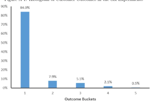
We summarize the distribution of outcomes by grouping the outcomes into five discrete buckets. The first bucket included the customers for whom profit was zero or negative. The customers in the next four outcome buckets all contributed positive profits. Because the profit levels are confidential we do not disclose the cutoff limits (recall that we only use these outcomes to provide the primitives to generate simulated data). In Figure A.1 we report a histogram of the customer outcomes across the six experiments. The unit of observation is a customer in an experiment and the columns add to 100%.

We use the outcomes from this experiment to provide primitives to generate a dataset to use for illustration. The dataset is generated from an MDP with five states and two actions: 𝑠 = {1, 2, 3, 4, 5} and 𝑎 = {0, 1}. The state in period 𝑡 corresponds to the profit earned from the experiment in period 𝑡. For example, if the outcome in period 𝑡 corresponds to the third outcome bucket, the state in period 𝑡 is State 3. The rewards 𝑅𝑀 : 𝑆 × 𝐴 → 𝑅, transition probabilities 𝑃𝑀 : 𝑆 × 𝐴 → 𝑆, and policy 𝜋𝑀 _{: 𝑆 → 𝐴 to generate this MDP are all correspondingly generated from}

the actual campaign experiment data.3

We constructed a RFM state space by discretizing the recency and frequency variables to three levels, and the monetary value variable to five levels. This yields

3_{The rewards are the midpoint of the profit earned in each of the discrete outcome buckets. If}

the outcome in period 𝑡 corresponds to the third outcome bucket, the rewards for that customer in period 𝑡 is equal to the midpoint of the rewards in that bucket. The transition probabilities for each state-action pair are calculated by counting the proportion of times a customer in that state that received that action (mail or not mail) transitioned to each of the other state in period 𝑡+1. Because the actions (mail and not mail) were randomized, the policy is a stochastic policy, and reflects the percentage of times a customer in that state received each action.

(27)

a state space with 45 states. At each period in the simulation data, we evaluate the RFM variables of each customer and assign the customer into the corresponding RFM state.

Because the data is simulated we know the true state space in this dataset, and so we can use standard methods to calculate the true weighted value function (we delay discussion of the methods until Section 6). When we use the true state spaces, the weighted value function estimate for policy 𝜋𝑀 is 15,039. However, when we use the RFM states, the value function estimate for the same policy becomes 20,161. This error is solely attributable to the design of the state spaces. Further investigation reveals that the RFM approach does not yield states that satisfy the Markov property. About 62.50% of the states constructed using the RFM method are Markov.

This illustration highlights the role that the design of the states can play in con-tributing to the error in RL methods. In Section 7 we will show that these errors can be greatly reduced if we design states that satisfy the Markov property. We next introduce the method that we propose for accomplishing this purpose.

(28)

(29)

Chapter 4 Main Idea of State Construction

The goal while constructing states is to create a mapping from the historical trans-action data to some manageable dimension space that satisfies the Markov property. What we propose is to map from the space of historical transaction data to probabil-ity space, representing predictions of how customers will respond to future marketing actions. The challenge is to find a set of events that are sufficient for the prediction of all other future purchasing events. We elaborate on this concept below.

4.1 State Representation

To understand our state representation idea, we need to introduce the concept of an observation, denoted by 𝑂. The firm’s interaction with its environment can now by described as: at each time period 𝑡, the firm executes a mailing action 𝑎𝑡 ∈ 𝐴 = {𝑁 𝑜𝑡𝑀 𝑎𝑖𝑙, 𝑀 𝑎𝑖𝑙} = {0, 1} and receives an observation 𝑜𝑡 ∈ 𝑂. Different

customers can receive different 𝑎𝑡, and the observation 𝑜𝑡 can be high-dimensional.

For example, observation 𝑜𝑡 can be a two-dimensional variable, with 𝑜1𝑡 corresponding

to the number of units a customer purchased at period t, and 𝑜2_𝑡 corresponding to the revenue from the customer’s purchase at period 𝑡. Observation 𝑜𝑡 can also include

customer characteristics, such as age, gender, and environmental variables measur-ing seasonality. Because the observation can measure purchasmeasur-ing, the current period reward (in an MDP) can be represented in the observation. For ease of exposition,

(30)

we will treat observation 𝑜𝑡 as a one-dimensional variable. Specifically, we assume

𝑜𝑡 ∈ 𝑂 = {𝑁 𝑜𝑡𝐵𝑢𝑦, 𝐵𝑢𝑦} = {0, 1}.

Suppose the firm is at time period 𝑡. An action-observation sequence is a sequence of alternating actions and observations. A history, denoted as ℎ = 𝑎1𝑜1𝑎2𝑜2. . . 𝑎𝑡𝑜𝑡,

describes the action-observation sequence that the firm has experienced from the beginning of time through period 𝑡. A test, denoted as 𝑞 = 𝑎1𝑜1𝑎2𝑜2. . . 𝑎𝑛𝑜𝑛, describes the action-observation sequence that might happen in the future. We define the predicted probability of a test (𝑞 = 𝑎1𝑜1𝑎2𝑜2. . . 𝑎𝑛𝑜𝑛) conditional on a history (ℎ = 𝑎1𝑜1𝑎2𝑜2. . . 𝑎𝑡𝑜𝑡) as:

𝑝(𝑞|ℎ) ≡ Pr{𝑜𝑡+1 = 𝑜1, 𝑜𝑡+2 = 𝑜2, . . . , 𝑜𝑡+𝑛 = 𝑜𝑛|ℎ, 𝑎𝑡+1 = 𝑎1, 𝑎𝑡+2= 𝑎2, . . . , 𝑎𝑡+𝑛 = 𝑎𝑛}

We will use an example to help illustrate the meaning of this probability. In an email (or direct mail) targeting problem, the firm observes whether each customer received each past email, and whether the customer bought in each past period. This is the history we refer to. For example, consider the test: (𝑞 = 𝑎1_𝑜1_𝑎2_𝑜2_{), where}

𝑎1 _{= 𝑎}2 _{= 1 and 𝑜}1 _{= 𝑜}2 _{= 1. The conditional probability 𝑝(𝑞|ℎ) represents the}

predicted probability that a customer bought in both period 𝑡 + 1 and period 𝑡 + 2, conditional on the customer’s past history and receiving an email at period 𝑡 + 1 and period 𝑡 + 2.

The central idea of Predictive State Representations (PSRs) is to choose a set of tests, and use the predictions of those tests to construct states. Suppose the set of tests has m elements, we can write this set of tests as 𝑄 = {𝑞1, 𝑞2, . . . , 𝑞𝑚}. Informally,

tests in 𝑄 can be understood as the prediction of future action-observation sequences. To be specific, we use the column vector 𝑝(𝑄|ℎ) = [𝑝(𝑞1|ℎ), 𝑝(𝑞2|ℎ), . . . , 𝑝(𝑞𝑚|ℎ)]𝑇 as

state representations for each customer. Customers with the same 𝑝(𝑄|ℎ) will be grouped into the same state.

The next question is how to choose the set of tests 𝑄 so that the states satisfy the Markov assumption. We require that 𝑄 is chosen so that 𝑝(𝑄|ℎ) forms a sufficient statistic for all future test predictions. More formally, for any test 𝑞, there exists an

(31)

(𝑚 × 1) vector 𝑚𝑞, such that1:

𝑝(𝑞|ℎ) = 𝑝(𝑄|ℎ)𝑇𝑚𝑞

Throughout the paper, we assume the existence of such a set of tests 𝑄, and call the tests in set 𝑄 as core tests. This is not a strong assumption as for any problem that can be represented by a finite POMDP or a k-history model, there exists a set 𝑄 with finite elements that can also represent the problem (Wingate 2012). Moreover, compared with a POMDP, the number of core tests is no larger than the number of hidden states in the POMDP model (Littman et al., 2001).

4.2 Properties of the Constructed State

We next explain why the PSR states satisfy the Markov property. Second, we show that the proposed state representation can be recursively updated.

Suppose we already have some historical data up to period 𝑡 for each customer, denoted as ℎ𝑖_𝑡for customer 𝑖. In our email setting, ℎ𝑖_𝑡 includes whether each customer received an email and bought at each time period before time 𝑡 (including period 𝑡). The state representation finds a compact summary of the historical data for each customer. A key insight is that: states that satisfy the Markov property contain the same amount of information about the probability of future purchases as the raw history data. Formally, if two customers (denoted as A and B) who have different histories, ℎ𝐴_𝑡 ̸= ℎ𝐵

𝑡 , are assigned to the same state group, they should share the same

probabilities for the next observation:

𝑃 𝑟{𝑜𝑡+1= 𝑜|ℎ𝑡 = ℎ𝐴𝑡 , 𝑎𝑡= 𝑎} = 𝑃 𝑟{𝑜𝑡+1 = 𝑜|ℎ𝑡= ℎ𝐵𝑡 , 𝑎𝑡= 𝑎}

If this holds for any customers who are assigned to the same state, we can say that the constructed states satisfy the Markov property. More generally, a Markov state should not only be good at predicting the next observation, but also any higher length

(32)

observations.2 The PSR approach is motivated by this insight. If we can find the correct core tests (future events) and accurately estimate the probabilities associated with these core tests, then the resulting states will satisfy the Markov assumption.

The equation above also suggests a test of whether a state satisfies the Markov property. The following conditional independence test provides a necessary (though not sufficient) test of whether a state is Markov: 𝑝(𝑜𝑡+1|𝑎𝑡) is independent of ℎ𝑡 for all

observations in the same state.3 This is the method we used to evaluate how many of the RFM states were Markov at the end of Section 3. We will also use this test to help evaluate our state construction method in Section 7.

We next show that the states constructed here can be easily updated. Consider a specific customer who has a history ℎ𝑡 up to period 𝑡. At period 𝑡 + 1, this customer

receives mailing action 𝑎𝑡+1 and makes purchasing decision 𝑜𝑡+1. We now have a

new history up to period 𝑡 + 1, ℎ𝑡+1 = ℎ𝑡𝑎𝑡+1𝑜𝑡+1. We can calculate the predicted

probability 𝑝(𝑞𝑗|ℎ𝑡+1) where 𝑞𝑗 ∈ 𝑄 by:

This state-update function is easy to estimate, and applies to all histories and all core tests. We next discuss the empirical construction of states from data.

2_{Notice also that different periods of a specific customer should be treated in the same way as}

different customers.

3_{This test only considers predictions of the next observation, while Markov states should be}

good at predicting any length future observations. However, this proposed test offers an important indication of whether a state satisfies the Markov property.

(33)

Chapter 5 Constructing States from Data

The discussion in Section 4 reveals that we need to do two things to learn states from data. First, we need to find the core-test set 𝑄. Second, we need to estimate the conditional probability 𝑝(𝑄|ℎ) for any possible ℎ. We conclude this section by providing a theoretical guarantee for our proposed approach.

5.1 Finding Core Tests

We first discuss how to find the core-test set 𝑄. This is a challenging task, and early attempts to solve the problem were not able to provide any theoretical performance guarantees (see for example James and Singh 2004 and Wingate and Singh 2008). We propose an adaptive approach based on James and Singh (2004) that exploits ideas from linear algebra (Golub and Van Loan, 2013). Our method, which is easy to understand and implement, exploits sparsity. As we discussed in the Introduction, a common feature of transaction data is that many customers do not purchase every period, and so the incidence of purchases is “sparse” (see for example the distribution of outcomes in Figure A.1). This feature will greatly simplify the process of finding core tests.

To understand our proposed approach, we introduce a new concept, the system dynamic matrix. The system dynamic matrix is a way to represent a sequential decision-making problem (without introducing any new assumptions). Consider an

(34)

ordering over all possible tests: 𝑞1, 𝑞2. . . . Without loss of generality, we assume that

the tests are arranged in order of increasing length. Within the same test length, they are ordered in increasing values of our binary outcome indicator.

We define an ordering over histories ℎ1, ℎ2. . . similar to the ordering over tests.

The difference is that we include the zero-length/initial history ∅ as the first history in the ordering. The system dynamic matrix is such that the column corresponds to all tests by ordering, the row corresponds to all histories by ordering, and the entries are the corresponding conditional probability 𝑝(𝑞|ℎ). An example is given in Figure A.2.

The core tests correspond to the linearly independent columns in the system dy-namic matrix. This means that to find the set of core tests 𝑄, we just need to find the linearly independent columns of the system dynamic matrix (which has infinite-dimension). If we know all of the matrix entries of the first row, we can get all of the other matrix entries using the state update relationship (which we presented at the end of Section 4). Specifically, we can obtain a specific entry of the system dynamic matrix through:

𝑝(𝑞|ℎ) = 𝑝(ℎ𝑞) 𝑝(ℎ)

Thus, if we know all of the matrix entries of the first row, we can get all of the other matrix entries using this state update relationship.

The difficulties are two folds. First, we do not know the true conditional prob-ability 𝑝(𝑞|ℎ). Instead, we need to estimate these probabilities from data. This introduces the potential for estimation errors, and these errors could make linearly independent columns appear dependent (it is also possible, though less likely, that dependent columns may become independent). Second, in practice the length of the available data is finite. For example, we used just six experiments in the example at the end of Section 3. Yet, we are trying to learn the independent columns of an infinite dimension matrix. Because of these data challenges, we can only hope to find approximately correct core tests.

(35)

We consider the problem in two steps. First, we will assume that the probabilities in the system dynamic matrix are known exactly, and consider how to find the linearly independent columns.

1. Delete history rows whose corresponding tests have zero probability at zero-length history. If a test has zero probability with zero zero-length history, it also has zero probability with longer history. The histories that are not deleted provide the rows of the submatrices used in the next steps.

2. Start from the submatrix containing all tests up to length one. Calculate the rank of this matrix, and the corresponding linearly independent columns.

3. Expand the submatrix to the one whose columns are the union of all length-one tests, the linearly independent tests found so far, and all one-step extensions of these independent tests.1

4. Calculate the rank and linearly independent columns of this new submatrix. 5. Repeat Steps 3 and 4 until the rank does not change.

Step 1 of this algorithm is where we exploit the sparsity that is common in trans-action histories. For example, in our implementation data, there are five observation levels and two action levels. This results in 10 length-one tests, 100 length-two tests, 1000 length-three tests, etc. We can see that the system dynamic matrix grows ex-ponentially. However, because transactions are sparse, our method will delete many history rows in Step 1. This greatly reduces the computational burden when we expand the submatrix in Steps 3, 4 and 5. In our application, the sparsity in the transaction data allows us to delete approximately 80% of the history paths, which leaves a computationally feasible submatrix.

We can also show that as the size of the system dynamic matrix increases, the level of sparsity grows at least as quickly.

1_{Given a test 𝑞, a one-step extension refers to a new test 𝑎𝑜𝑞, where 𝑎 ∈ 𝐴 = {0, 1} and}

(36)

Result 1. The zero history rows (sparsity) grow exponentially as the history length increases.

Proof : If a test 𝑞′ has zero probability at zero-length history, all one-step ex-pansions of test 𝑞′(𝑞′𝑎𝑜), and extensions of test 𝑞′(𝑎𝑜𝑞′) have zero probability at zero-length history. If we imagine an infinite dataset, zero probability of test 𝑞′ at zero-length history means that we will not observe any pieces of 𝑞′ in this infinite dataset. Thus, any pieces of 𝑞′𝑎𝑜 and 𝑎𝑜𝑞′ will not exist in this infinite dataset. Thus, the “sparsity” will also grow exponentially. More importantly, it grows at a faster rate than the growth rate of the system dynamic matrix.

This result is important. It increases confidence that our proposed algorithm for finding core tests will continue to be computationally feasible as the size of the system dynamic matrix grows.

Recall that we have focused on cases in which we know the probabilities in the system dynamic matrix exactly. If we continue to make this assumption we can provide a guarantee on the performance of the algorithm.2

Result 2. The core tests identified using this 5-step algorithm are correct if all entries in the system dynamic matrix are known exactly.

Proof : See Appendix.

This result guarantees that the core tests obtained using this method are correct. We will label these linearly independent rows as “core histories”.

In practice, there are likely to be estimation errors in the probabilities in the system dynamic matrix. This can raise several issues. First, it can influence how we obtain the rank and linearly independent columns in Steps 2 and 4. We relegate a discussion of these details to the Appendix. Second, it becomes more difficult to provide a guarantee on the performance of the method. To do so we need an asymptotic result that as the time-period (denoted as 𝑇 ) of the data increases to

2_{If we know the probabilities in the system dynamic matrix exactly, another implication is that}

if a test 𝑞′ has zero probability at zero-length history, test 𝑞′ will not be one of the core tests. The

reason is that for any history ℎ, 𝑝(𝑞′|ℎ) will be zero. It seems that then we can exclude 𝑞′ in our five-step algorithms. However, we choose not to do this because under our probability estimation method

(introduced in next subsection), 𝑝(𝑞′|ℎ) may not be zero even if 𝑝(𝑞′|∅) is zero. This adjustment

(37)

infinity (𝑇 → ∞), the set of core tests we find are close to the true core tests. The result will not hold if we consider a general matrix structure. However, one feature in the customer transaction behavior can help with this asymptotic result.

The observation is that customers’ purchase behavior will not depend on events that happened infinite time ago. In practice, there will generally exist a time 𝑇0

(which can be very large) such that customers’ purchase behavior at most depend on 𝑇0 time ago events. The implication is that all histories with length higher than

𝑇0 have the same predicted probabilities of all future events as the corresponding

length-𝑇0 histories. Thus, if we have enough time period data, that is, 𝑇 ≥ 𝑇0, we

will find the correct core tests using our five-step algorithm based on Result 1. We will also demonstrate in Section 7 that the states that we design using the core tests behave well in practice.

Our discussion of the theoretical properties of this method has also been based upon the assumption that we can learn the entries in the system dynamic matrix exactly. In reality, we need to estimate these probabilities from a finite sample of data. We leave the issue of how to estimate the predicted probabilities 𝑝(𝑞|ℎ) until the next subsection.

We finish the discussion in this subsection with two additional comments. First, while the five-step algorithm and Results 1 and 2 are both new, we want to acknowl-edge that they build upon a similar method proposed by James and Singh (2004). A difference is that James and Singh (2004) propose submatrix expansion on both histories and tests in each iteration (we just expand the tests). This method is not guaranteed to find the correct core tests even if all entries in the system dynamic matrix are known. Their method also faces computation challenges, which we alle-viate by exploiting the sparsity in customer transaction data. Wingate and Singh (2008) propose using randomly selected tests as core tests, but this approach is also not guaranteed to find the correct core tests.

Second, the approach we propose may have difficulties dealing with tests that have long lengths. We discuss this issue in Section 8.

(38)

5.2 Calculating Predicted Probabilities

Once we obtain the core tests, we can derive the state for each customer at each period by calculating the (conditional) probabilities of the core tests. Customers with the same probabilities will be assigned to the same state group. Estimating these probabilities from data is conceptually straightforward, but there are several details that deserve comment.

The goal is to estimate the predicted probabilities 𝑝(𝑞|ℎ) for the core tests. A straightforward approach is to simply count how many ℎ and ℎ𝑞 appear in the dataset, and then take the fraction of ℎ𝑞 over ℎ.3 _{For example, suppose ℎ = “01” = {𝑎}

1 =

𝑁 𝑜𝑡𝑚𝑎𝑖𝑙, 𝑜1 = 𝐵𝑢𝑦} and 𝑞 = “11” = {𝑎1 = 𝑀 𝑎𝑖𝑙, 𝑜1 = 𝐵𝑢𝑦}. Then we can just

count how many times “01” and “0111” appear in the dataset, and calculate the “0111” occurrences as a proportion of “01” occurrences.

In order to do this, we need to define time period 0. Notice that in our method, each period’s data has a different length of history. This makes the definition of time period 0 important, because the calculation of the probabilities could be sensitive to the choice of starting time. Moreover, if we define time period 0 to always start with the first time period in our data, we will place more reliance on the data at the start of our data period, which places more reliance on the least recent data. This could make our estimation very sensitive to non-stationarity.

To address this concern, we propose the following sampling method. Suppose we have data on T periods and N customers. We divide the N customers randomly into M groups, and for each group we randomly assign time period 0 to different calendar time periods. Each of the customers in the same group are assigned the same calendar time period as period 0, but different groups are assigned different calendar time periods as period 0. For example, recall the six email experiments described at the end of Section 3. There were 136,262 customers that participated in all six experiments. We would randomly divide these customers into six groups. In

3_{It is possible that the length of ℎ𝑞 is larger than the total time period in the data. For this}

reason, when we search for the core tests, we restrict attention to submatrices for which we can directly estimate the predicted probabilities 𝑝(𝑞|ℎ).

(39)

one group, period 0 would correspond to the first experiment, another group would treat experiment two as period 0, etc. For the customers for which experiment two is period 0, period 1 would be experiment 3, period 2 would be experiment 4, and so on. The benefit of this approach is that it ensures the estimated probabilities are less sensitive to temporal variation in outcomes. A limitation is that we do not use all of the data; in groups for which there are experiments before Period 0, we do not use these earlier experiments to estimate the probabilities.

Notice that we use the predicted probabilities in the system dynamic matrix in two stages: (a) to find the core tests in the system dynamic matrix, and (b) after finding the core tests we group customers into states according to the conditional proba-bilities associated with these core tests. We can either re-use the same assignment of customers to period 0 in both places, or we can re-sample after finding the core tests (to re-allocate period 0 across customers). In our implementation, we choose to resample. This has the advantage of reducing the relationship between estimation errors in the two stages. However, it may also increase the risk that random variation results in breaches of the Markov assumption in some states.

Using our data, we can observe which tests happen after which histories. For example, suppose we have a dataset with 3 time periods. Consider a specific customer A who is assigned so that period 0 is the first period in the data. Suppose the data we observe for customer A is “011100”= {𝑎1 = 𝑁 𝑜𝑡𝑚𝑎𝑖𝑙, 𝑜1 = 𝐵𝑢𝑦, 𝑎2 = 𝑀 𝑎𝑖𝑙, 𝑜2 =

𝐵𝑢𝑦, 𝑎3 = 𝑁 𝑜𝑡𝑚𝑎𝑖𝑙, 𝑜3 = 𝑁 𝑜𝑡𝑏𝑢𝑦}. For customer A, after history ℎ ="01", tests

𝑞 ="11" and 𝑞 ="1100" are observed. For some tests our data length is too short to observe whether the test succeeds or not. In these situations, we use the predicted probabilities, which we can estimate using the state-update function (provided at the end of Section 4).4

Probabilities are continuous numbers. Unless we round the probabilities, we may not find two observations in the same state. The key to the use of rounding is that we need to do all probability approximation before we start identifying the core tests.

4_{To use the state-update function, we also need to know the parameter vector 𝑚}

𝑞 for test q.This

vector can be obtained through 𝑝−1(𝑄|𝐻)𝑝(𝑞|𝐻) where H includes all possible histories. We calculate

(40)

In this way, our rounding does not interfere with the Markov property of the states. If we round the probability after we derive the core tests, we risk introducing errors that may breach the Markov assumption in some states.

Finally, we may encounter covariate shift. Covariate shift arises if the distribution of the data used for training a targeting model is different than the data used for implementation (see for example Simester et al. 2019b). In our setting, the probability vector at the last period, which will guide the targeting policy in a sequential targeting problem, might not occur in any prior period. For those probability vectors, we have no observed outcomes. To address this issue, we assign customers with these probability vectors (in the last period) to the nearest state.5

In this section we have discussed how to use a sample of historical transaction data to create Markov states. In the next section we (briefly) discuss how standard Reinforcement Learning methods can use these states to estimate value functions and identify optimal policies.

(41)

Chapter 6 Dynamic Optimization

Recall that in the Introduction, we mention four steps in a standard Reinforcement Learning algorithm. Given that we have designed a discrete state space (the first step), we now discuss the remaining three steps. There are many standard methods to use for these steps. Because this is not the focus of the paper, we use the simplest approach, which is easy to understand and implement. This method also has well-established theoretical guarantees.

6.1 Estimating Current Period Rewards and

Transi-tion Probabilities

Just as the runner in baseball needs to know the transition probabilities from one state to another state for both “not steal” and “steal” actions, we need to estimate the transition probabilities for both the “mail” and “not mail” actions. In terms of an MDP, we need to estimate the stochastic transition probabilities 𝑃 : 𝑆 × 𝐴 → 𝑆.

We use a simple nonparametric approach to accomplish this. For each state and mailing decision, we observe from the historical data the proportion of times customers transitioned to each of the other states. The benefits of this approach are discussed in detail in Simester et al., (2006).

(42)

6.2 Estimating the Value of Each State for a Given

Policy

This step is normally called “Policy Evaluation” in the Reinforcement Learning liter-ature. In our baseball example in the Introduction, the number of expected runs in States 1, 2 and 3 were calculated as a simple average of the number of runs scored from the states in past Major League Baseball games. However, these outcomes de-pend upon how the game will be played in future states. In particular, the value function under an arbitrary policy 𝜋(𝑠) can be written as:

𝑉𝜋(𝑠) = 𝐸𝑟,𝑠′[𝑟(𝑠, 𝜋(𝑠)) + 𝛿𝑉𝜋(𝑠′)|𝑠, 𝜋(𝑠)]

We adopt the notation introduced in Section 3. Suppose we use 𝑟(𝑠, 𝑎) to represent the expected rewards in state 𝑠 when the firm chooses mailing action 𝑎, then we can rewrite the value function as:

𝑉𝜋(𝑠) = ˜𝑟(𝑠, 𝜋(𝑠)) + 𝛿∑︁

𝑠′

𝑝(𝑠′|𝑠, 𝜋(𝑠))𝑉𝜋(𝑠′)]

With a slight modification of notation, we can express the above equation in vector form. Let 𝑉𝜋 _{denote the vector with elements 𝑉}𝜋_{(𝑠), 𝑟}𝜋 _{with elements 𝑟(𝑠, 𝜋(𝑠)) and}

𝑝𝜋 _{(a matrix) with elements 𝑝(𝑠}′_{, 𝜋(𝑠)). Thus, 𝑉}𝜋 _{= 𝑟}𝜋 _{+ 𝛿𝑝}𝜋_𝑉𝜋_{, and we can obtain}

the value of each state under an arbitrary policy from 𝑉𝜋 _{= (𝐼 − 𝛿𝑝}𝜋₎−1_𝑟𝜋_.

To estimate 𝑉 (𝑠), we also need to estimate the one-period expected rewards 𝑟(𝑠, 𝑎) for each state-action pair. Similar to estimating the transition probabilities, we es-timate the one-period rewards using a simple nonparametric approach; we calculate the average one-period reward for each state and mailing decision.

(43)

6.3 Choosing the Optimal Policy

In our baseball example, the runner chooses the optimal action in state 1 using the value function estimates associated with the two state-action pairs in state 1: the runner only steals if 0.5088 < 0.6675 * 𝛽 + 0.0986 * (1 − 𝛽). When there are many states, for any given policy we can calculate the value function for each state-action pair. We can then improve the policy by choosing the action with the highest value in each state.

Notice that when we change the policy (the “Policy Improvement” stage) this recursively changes the value function estimates for each state-action pair, and so we must then re-evaluate the improved policy (the “Policy Evaluation” stage). We can then try to further improve the policy. This is the idea behind the classical policy-iteration algorithm, which we use in this paper to find the optimal policy. If the current policy already chooses the action with the highest value in each state then the current policy is optimal.

In practice, the policy-iteration algorithm starts with any arbitrary policy for which we estimate the value function. We use this value function to improve the policy, which yields a new policy with which to begin the next iteration. The sequence of policies improves monotonically until the current policy is optimal. The policy-iteration algorithm is guaranteed to return a stationary policy that is optimal for a finite state MDP (Bertsekas, 2017). However, this guarantee only holds if the states satisfy the Markov property.

In the next section we validate our proposed method for constructing states by investigating whether it is robust to the introduction of non-Markov distortions in the data.

(44)

(45)

Chapter 7 Validation

We start by describing our validation approach. The first set of results investigate the robustness of our method to non-Markov distortions in the state space used to generate the data. We then investigate the impact of errors in the estimated (con-ditional) probabilities. Finally, we evaluate the proposed approach using model-free field data.

7.1 Validation Approach

We design a validation environment in which any error in the design of the state space is solely attributable to non-Markov distortions that we control. We start by describing a state space that does not have any non-Markov distortions. We then introduce two types of distortions; distortions in either the current period rewards, or distortions in the transition probabilities.

We return to the simulated dataset that we discussed in Section 3. Consistent with the discretization of the outcomes in each time period, we consider an MDP with five states and two actions: 𝑠 = {1, 2, 3, 4, 5} and 𝑎 = {0, 1}. The reward 𝑅𝑀 _{: 𝑆 × 𝐴 → 𝑅, transition probabilities 𝑃}𝑀 _{: 𝑆 × 𝐴 → 𝑆 and policy 𝜋}𝑀 _{: 𝑆 → 𝐴}

to generate the MDP are all constructed from the actual experimental data. Details are discussed in Footnote 4.

(46)

fol-lows:

∙ With probability 𝛼, the state at time period 𝑡 is determined by the state at time period 𝑡 − 2 : 𝑃𝑀(𝑠𝑡|𝑠𝑡−2, 𝑎𝑡−1); and

∙ With probability 1 − 𝛼, the state at time period 𝑡 is determined by the state at time period 𝑡 − 1 : 𝑃𝑀(𝑠𝑡|𝑠𝑡−1, 𝑎𝑡−1).

With probability 1 − 𝛼 the transition probabilities only depend upon the state in period 𝑡 − 1 and so the states 𝑠 = {1, 2, 3, 4, 5} satisfy the Markov property. However, with probability 𝛼 the transition probabilities depend upon the state in period 𝑡 − 2 and so the states 𝑠 = {1, 2, 3, 4, 5} do not satisfy the Markov property.

To introduce non-Markov deviations in the rewards we use a similar approach: ∙ With probability 𝛼, the reward at time period 𝑡 is determined by the state at

time period 𝑡 − 1 : (𝑅𝑀_𝑡−1(𝑠𝑡−1, 1) + 𝑅𝑀𝑡−1(𝑠𝑡−1, 0))/2; and

∙ With probability 1 − 𝛼, the state at time period 𝑡 is determined by the state at time period 𝑡 : 𝑅𝑀_𝑡 (𝑠𝑡, 𝑎𝑡).

We present results using data generated under different values of 𝛼. In particularly, we allow to vary from 0 to 0.9 in increments of 0.1, and separately evaluate deviations in the rewards and the transition probabilities. For each value of , we simulate a dataset with 200,000 customers and 8 time periods.

We compare two state space designs: Benchmark the five states in the MDP: 𝑠 = {1, 2, 3, 4, 5}; Our Method states generated using the method proposed in this paper. Because the Benchmark state space uses the five states in the data-generating MDP, we can isolate the effects of non-Markov deviations on the value function estimates. If we use other methods to generate states, we cannot isolate whether errors are due to the non-Markov distortions, or from other failings in the state space design. We expect that the performance of the five Benchmark states should worsen as the parameter increases due to the introduction of the non-Markov distortions. In contrast, the states generated by the method proposed in this paper

(47)

should be robust to non-Markov distortions, and so the results should be stable when 𝛼 increases.

7.2 Validation Results Using True Probabilities

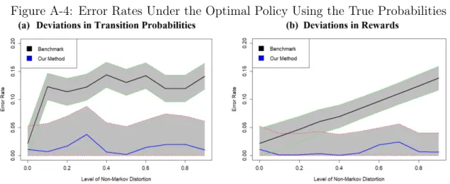
We first present results using the true probabilities used to generate the simulated data. We also initially focus on the “current policy” reflected in the data (recall that this policy was randomized). We will later also investigate how well the state space designs perform when they are used to design “optimal” policies.

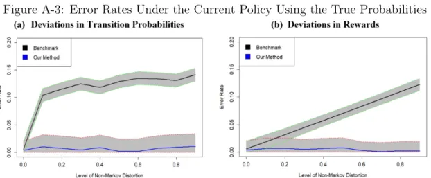
In Figure A.3 we report the error rates of the estimated value functions. For both state space designs, we weight the value function estimates for each state by the number of visits to each state in the data. Our error measure is the absolute difference in the average performance compared to the true value function estimate. In the datasets with deviations, the true value function estimate is calculated using a state space with 25 states to account for whether the transitions (or rewards) depend upon period 𝑡 − 1(𝑡) or period 𝑡 − 2(𝑡 − 1) (this is a 1-history state space). Standard deviations are estimated using the method proposed in Mannor et al., (2007). The shaded areas in the figure identify 95% confidence intervals.

In Figure A.3 we see that, without any deviations, both state spaces perform well and yield value function estimates for the current policy that are close to the true values. However, with the introduction of distortions in the transition probabilities, there is an immediate and large deterioration in the accuracy of the benchmark state space. The reduction in accuracy is dramatic even for 𝛼 = 0.10. This deterioration is completely attributable to the non-Markov distortions, and highlights the cost of breaching the Markov assumption in the design of state spaces. The performance continues to deteriorate as the size of the distortions increases beyond 𝛼 = 0.10. In contrast, while there is some volatility, the overall performance of the proposed method is relatively robust to the non-Markov dynamics in the data.

We observe a similar pattern when we investigate deviations in the rewards. How-ever, an important difference is that the performance of the benchmark method

Dynamic marketing policies : constructing Markov states for reinforcement learning

Dynamic Marketing Policies: Constructing Markov States

for Reinforcement Learning

Dynamic Marketing Policies: Constructing Markov States for

Reinforcement Learning

by

Yuting Zhu

Abstract

Contents

List of Figures

List of Tables

Chapter 1

Introduction

Chapter 2

Literature Review

Chapter 3

Criteria for Designing States

3.1

States and MDPs

3.2

MDPs and Targeting

3.3

Illustration of the "RFM" Approach

Chapter 4

Main Idea of State Construction

4.1

State Representation

4.2

Properties of the Constructed State

Chapter 5

Constructing States from Data

5.1

Finding Core Tests

5.2

Calculating Predicted Probabilities

Chapter 6

Dynamic Optimization

6.1

Estimating Current Period Rewards and

Transi-tion Probabilities

6.2

Estimating the Value of Each State for a Given

Policy

6.3

Choosing the Optimal Policy

Chapter 7

Validation

7.1

Validation Approach

7.2

Validation Results Using True Probabilities