Distributed routing

by

ART O'LEARY

SUBMITTED IN PARTIAL FULFILLMENT OF THE REQUIREMENTS OF THE

DEGREE OF

DOCTOR OF PHILOSOPHY

at the

MASSACHUSETTS INSTITUTE OF TECHNOLOGY January 1981

Massachusetts Institute of Technology

Signature of AuthorI -w =

Department of Electr'al Engineering and Computer ScieniT, January 13, 1981 Certified by

Robert G. Gallager Thesis Supervisor Accepted by

Arthur C. Smith, Chairman Department Committee on Graduate Students

DISTRIBUTED ROUTING by

ART O' LEARY

Submitted to the Department of Electrical Engineering and Computer Science

on January 13, 1981 in partial fulfillment of the requirements for the degree of Doctor of Philosophy.

ABSTRACT

In distributed routing each node receives some information about the network from its adjacent nodes and uses the infor-mation to determine the manner in which it forwards its

traffic. This thesis gives three examples of distributed routing in a data communication network. A routing algorithm

is then given where a generalized distributed routing pro-cedure proposes a flow change and a central node determines the optimal scale of the. proposed change. Small flows on long and unwanted paiths are set to zero regardless of the scaling. The thesis shows that the iterative use of this algorithm converges to the optimal network cost, e.g. it minimizes the mean delay.

Thesis Supervisor: Robert G. Gallager

Title: Professor of Electrical Engineering and Computer Science

Table of Contents

Page

Chapter I. Introduction 4

1.1 The Routing Problem 6

1.2 A Distributed Routing Algorithm 9

Chapter II. Second Order Routing 16

2.1 Notation 16

2.2 An Algorithm Using Second Derivatives 19 2.3 An Algorithm Not Using Second

Derivatives 27

Chapter III. Partially Distributed Routing 42

3.1 A Generalized Algorithm with Scaling 43

3.2 Convergence 50

Appendix A. Dual of the Routing Problem 74 A.1 Linear Programming Application 74

A.2 Error Bound 78

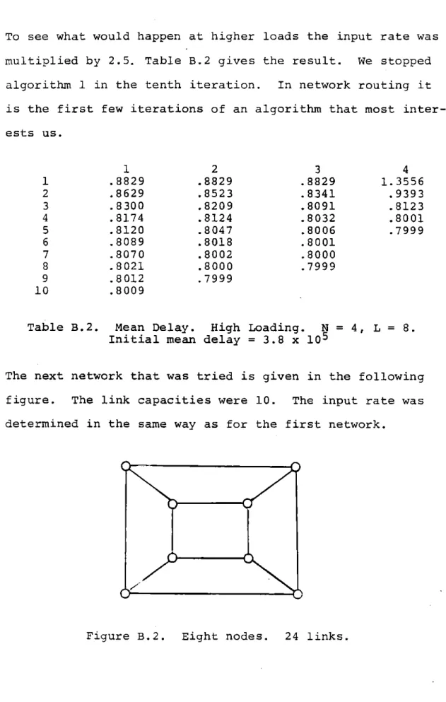
Appendix B. Routing Samples 79

Chapter I. Introduction

Many computer centers share their resources through some communication linking. For economic reasons most pairs of computer centers are not directly linked so a message or file often travels over several links to get to its destination. For operational reliability most source-destination pairs are connected with two or more distinct message paths.

The choice of which path a message is to follow is a routing decision. This decision might be to use the path with the smallest number of links, provided it is not con-gested. If the delays resulting from queuing at the computer centers and transmission across the links are significant, then the routing decision might be to use the path with the

shortest delay.

These routing decisions require some knowledge of the network. In centralized routing one computer center (with perhaps several backup centers) takes the responsibility of monitoring the network. This center receives the status of the links and the size of the traffic flow from each source to each destination. It sends out to the other centers their routing instructions.

In distributed routing, each center determines the best route based on the status of the adjacent links and on its neighbors' estimates of their distances (number of links, the delay, or whatever) from the destination. More details are

given later.

Our basic routing criteria is that the routing should minimize a network cost function. The specific form of this

function is given in the next section. The mean delay is a common example of the network cost.

Iterating a routing algorithm should lead to the optimal routing whenever the traffic from each source to each destina-tion is constant. Gallager [77] gave the first distributed routing algorithm that satisfies this criteria. Bertsekas

[78] and Gafni [79] generalized Gallager's algorithm and gave different proofs of convergence.

In contrast to centralized routing these distributed

algorithms are often guaranteed to converge only if the routing changes are small at each iteration. Presumably, the conver-gence is also slower than that of centralized algorithms. In chapter three we describe a distributed routing algorithm in which the routing changes are comparable to those of a cen-tralized routing algorithm.

In order to maintain a good routing when the source-destination traffic slowly changes, the routing algorithm is periodically iterated. An algorithm with a good convergence rate should need fewer iterations to give a good routing. If the traffic changes more rapidly, then the algorithm is iterated more often. In the extreme case, the traffic changes so rapidly that the algorithm cannot cope with it.

Empirical tests with a specific network are required to determine how often a routing algorithm should be iterated.

Rudin [80] suggests that these tests should take into account the control used to limit the traffic into the network. Under this flow control a good routing algorithm allows more traffic to enter the network.

The rest of this chapter details our routing problem and gives a simple distributed routing algorithm. The second

chapter gives two distributed routing algorithms that make the quadratic approximation of the change in the network cost non-positive. This means that the flow change generated is likely to make the cost function decrease. The third chapter gives a class of routing algorithzs in which the network control center is called upon to determine the size of the flow change. The third chapter also shows that this class converges. Appen-dix B illustrates some sample behavior of the algorithms

mentioned in the thesis.

1.1 The Routing Problem

Let N be the set of nodes (switching centers). A duplex communication channel between nodes i and j is interpreted as a pair of directed links (i,j) an& (j,i). Let L be the set of directed links.

We will call the traffic destined for node k commodity k and we will let C denote the set of commodities.

The instantaneous description of the network consists of the number of bits of each commondity travelling on each link and the number of bits of each commodity waiting at each node for transmission over a link. This instantaneous description

is of little use for routing as during the time it takes a node to describe to its neighbors the state of its queues, the queue lengths usually change significantly.

A less volatile description of the network is the average rate over a given time interval at which each commodity travels over each link and the average rate at which each queue length changes. If the time interval is large enough then, because the queue lengths are finite, the latter rates will be small compared to the former. For example, in ten seconds 500,000 bits might be sent over a link while the queue length at the head of the link changes by 5000 bits. The average rate of change of 500 bits per second in the queue is small compared to average transmission rate of 50,000 bits per second on the link. Consequently, we will treat the rates at which the queue lengths change as zero.

k

Let F.. be the average rate at which commodity k travels '3

over link (i,j). F.k. is non-negative. Let f.. be the

aggre-iJ 13

k

gate flow on link (i,j), i.e., f. =SkF . Let c. .be the

capacity of link (i,j). Let R be the average rate at which k

commodity k originates at node i. Rk is non-negative for i4k. The consumption of commodity k at node k implies

R :=-E Rk keC (1.1.1)

k i/k i

The conservation of each commodity at each node and our treatment of the queue lengths as zero gives

Z.Fk -EZ Fk. + R ieN, keC (1.1.2)

The network cost will be taken to be the mean transmission cost - E .. .. . (f .. 1 1 3 r i 13 13 13 where r :=~ ki/k i

t. (f .) might be 1, representing the unit use of link (i,j) in which case the network cost is the mean hop length.

Alter--l

nately, t. . (f ..) might be (c. . - f ..) which is a standard

13 1-3 J1J 13

approximate formula for the mean delay on link (i,j) in a store and forward network [Cantor and Gerla 74]. We will write the network cost as

J(f) . .J. .(f. .) (1.1.5)

The link cost J. .(f..) is a function of the flow on that link. Our routing problem formulation is

minimize E. .J. .(f..) k subject to f. . = kF ij k ij k k k m im n ni=Ri f..< c.. 13 - 13 F.. > 0 13 (i,j)eL, keC (11(1.1.6)

The set of feasible flows is defined to be the set of varia-bles f,F that satisfies the constraints of (1.1.6). This

thesis assumes that on the set of feasible flows the network cost is twice continuously differentiable with positive partial derivatives and non-negative second partial derivatives.

Almost all of the results about the routing alogrithms in chapters two and three hold only when the input flow R is

constant. Rather than preface many remarks with the clause, "Assuming R is constant...," we here assume that R is constant in the rest of the thesis.

As stated in appendix A, the optimal flow of (1.1.6) is the one in which the flow travels along the path of the least incremental cost. If the derivative of J. . (f..) is taken to be the distance of the link (i,j) then the optimal flow is a

shortest distance flow. We denote this link distance as

DJ. .(f..)

g. . 1J:=(ij)eL (1.1.7)

13 39f..

By our assumptions about the network cost function we have

g. . > 0 (i,j)eL (1.1.8)

1.2 A Distributed Routing Algorithm

We introduce the basic details of distributed routing with the following routing algorithm. Recall that commodity k is the flow destined for node k. As we often describe what is happening one commodity at a time, we will just as often find

(j,i)es then we say that

j

is a neighbor of i.

In the following algorithm every node has a favored neighbor for each commodity. Initially, we let this be the neighbor on any path with the fewest links to the destination. For each commodity, V. is the distance from i to the destina-tion via the favored neighbors. Each node i selects as its new favored neighbor the neighbor m that minimizes gi.+V .

(gi is given in (1.1.7)). (We will later show that the new favored neighbors determine a tree directed into the destination.)

The proposed flow F' is the one that travels to the destination via the new favored neighbors. The new flow generated is that

convex combination of the present flow and the proposed flow that minimizes the network cost.

The following describes one iteration of the algorithm. We assume that the initial flow is feasible.

I. The following steps are done for each commodity.

A. The destination sends the signal "Vdest = 0" to

its neighbors.

B. Each node i waits until it receives Vn from its favored neighbor n. Then node i sends the follow-ing to its neighbors.

V. = _i g.n + Vn_{in n}

C. Each node i waits until it receives V. from every 2

neighbor

j.

Then it waits until it receives F!.

from every neighbor

j

for which V. > V.. Node i J1

automatically assumes F!. = 0 for those neighbors

J3

j

for which V. < V. Node i then determines its

J - i

new favored neighbor m by

m = arg-min {g..+V.} J

The proposed flow is F! = E F. + R. and

F!. = 0 if

j/m.

F!. is sent to node

j

if

13 1J

V. > V..

1 J

II. Each node i sends the set {f!.(=E F!k)} to every node. 3j k ij

III. Every node determines the y, 0 < y < 1, that minimizes

J((l-y)f+yf') while satisfying (1-y)f+yf' < c. For

each commodity and link (i,j) the new flow is

(1-y) F.. + yF! ..

In that last step a central node could receive f', determine y, and send this information out to all nodes. This would reduce the communication overhead, but would also introduce a delay before every node learns the value of y.

We now briefly check that the above algorithm generates a feasible flow. For each commodity and each node i we have for the n and m of step B and C,

V. =g. + V

V " in n

> g + Vm

(1.2.1) >mV

where the last inequality comes from (1.1.8). Thus, the new favored neighbors determine a tree rooted into the destination. The proposed flow travels on this tree and satisfies all of the constraints of (1.1.6) except, possibly, f' < c. Then, since

f is feasible, any flow satisfying (1-y)f + yf' < c with

0 < y < 1 is feasible. This shows that the algorithm is feasible.

When the link costs depend on the flow and the network is moderately to heavily loaded, the optimal flow usually has branches, i.e., multiple paths. In this situation a routing algorithm should not only indicate which path the flow is to be shifted to but also how much of the flow is to be shifted. The routing algorithms of chapter two do this job.

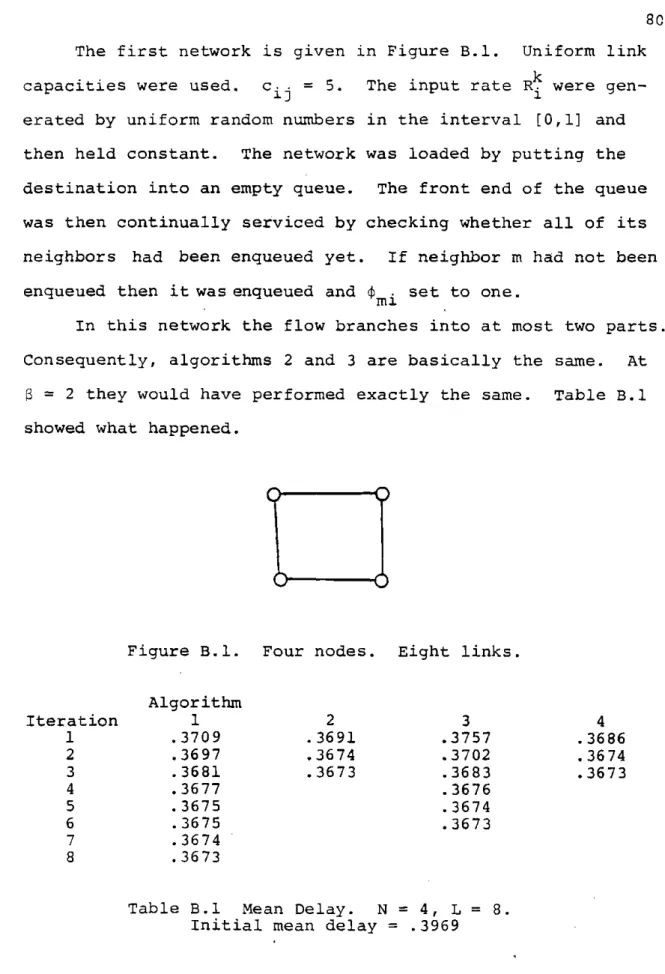
We end this chapter with an example. We start with the network of figure 1.2.1 and use only one commodity, that des-tined for node d. The link capacities are c.. = 5. The input flows are Rl = 3, R2 = 2, (and Rd = -5). The sum of the input flows is r = 5. The link cost functions are

f..

J (f ) = 1 1] (1.2.2)

ij ij 5 " 5-f. .

For the initial flow we have Fld = 3, F2d = 2. With the

following

9J. .(If. .)

'i1 =i 1 ,1(1.2.3)

af..2 '

iJ (5-f..)

we have for the initial flow, gid = 1/4, 92d = 1/9 12

V2 = 1/9. Node d remains the favored node of 2. Node 2

becomes the favored node of 1 because 1/4 >.1/25 + 1/9. The

proposed flow is F 3, F = 5. In step II, the optimal

12

2d

y will be found to be .3232. The new flow turns out to be the optimal flow with cost .4178. The initial flow had .4333 for its network cost. If each node had minimized its delay from the destination then the scaling y above would have been .4398 and the resulting network cost is .4198.

3 2.

2

d

Note l.N.l. Schwartz and Stern [80] summarizes the routing schemes used in present day networks. None except ARPANET uses distributed routing. Many do have distributed communi-cation for notificommuni-cation of congestion. In response to conges-tion, these networks change the routing to some predetermined path. None of the networks optimizes the network delay. The network that comes closest to this is the ARPANET [McQuillan

et alia, 80]. It takes the present delays in the network, finds the paths with the smallest delay (not incremental delay) and uses these paths ignoring the fact that the new routing would change the link delays.

Note l.N.2. For centralized routing there are many techniques to find the optimal routing. Among them are Cantor and Gerla

[74], Frank and Chou [71], the flow deviation method [Fratta, Gerla, and Kleinrock 73] and Schwartz and Cheung [76]. The

routing algorithm given in section 1.2 is a distributed

approximation of the flow deviation method. In the exact flow deviation method the proposed flow F' is sent down the path with the shortest distance wrt g.

Note l.N.3. Agnew [76] indicates that the difference between using the paths with the shortest delay and using the paths with the shortest incremental delay is largest at medium loadings. Rudin [80] indicates that the effect of using frequent routing determinations is most beneficial at medium loadings. The reason is that at low loadings the flow usually

follow the path with the fewest links. At high loadings, the hightst cost links form a cut set and the routing either avoids the cut set or balances the flow through the cut set so that the cost of the links are about the same.

Note l.N.4. Our routing criteria is that the routing should become optimal if the source-destination traffic remains

con-stant. Since this traffic changes one might try to improve on the routing in between routing determinations. Rudin [76] reports some benefit in using something close to the actual delay to the neighbor plus the reported delay from the neigh-bor to the destination in determining the shortest path. One might also predict the interim delay as a function of the flow sent to the destination by means the second derivative methods of chapter two in this thesis.

Chapter II.

Second Order Routing

The routing algorithms of this chapter generate a flow change F that reduces the quadratic approximation of the cost change. The convergence of these algorithms is covered in the next chapter.

2.1 Notation

We will be using the vector version of formulation (1.1.6) given in the first chapter along with some new quantities.

Let N be the number of nodes, L be the number of links, and

C be the number of commodities. From section 1.1 we have

k k

C=N. The commodity flow F is Lxl and the input flow R is

Nxl. For the most part we work with one commodity so it will be convenient to let F and R be the flow of a fixed commodity. The destination of this commodity will be called node dest.

Let the following NxL node-link incidence matrices be defined. +{1 if n=i n,ij _{0 if n#i} 1 if n=j E = neN, (i,j)eL (2.1.1) n,ij _{0 if n/j} E . . := E+ . . - E - . n,ij n, n

The conservation equation (1.1.2) is then EF = E F+R. Let the node flow T be defined by

T := E+F = E F + R (2.1.2)

T is Nxl. A routing variable $ is defined to be any non-negative LxN matrix that satisfies

f

l if n=i/dest

jij,n

{

0if n/i, i=dest, or n=dest (i, JeL, neN

(2.1.3)

Let the routing fraction be any (usually unique) routing variable such that if TQ#0 then .. . = F. ./T.

13,11J 1

If $.. is taken to be the row of $ that corresponds to link (i,j), then from the definition of a routing variabler$P. is non-zero only at O.. .. We have F.. = ..T = .. . T..

J]1 J 1J 1J,1 1

It will be convenient to take

4..

to be the element $.

1J lJ,i*

Then F. . = p. .T. . We will take O. to be the column of $ that

1J J1 1

corresponds to node i. The non-zero elements of ).T i are the flows that leave node i.

F = 4T (2.1.4)

Let F be a change in F. Let F' = F + F be the new flow after making the change. Let T' and $' correspond to F'.

Let T = T' - T and $ = 4' - $. From (2.1.2) and (2.1.4) we have the basic equations involving these quantities. As discussed near the end of section 1.1, R is assumed to be constant.

T' = E+F' = E~F' + R (2.1.5)

T = E F = E F (2.1.6)

F 'T'- OT _(2.1.8)

= tT + tT + $T _(2.1.9)

The last equation comes from the expansion of $' and T' in the previous equation.

The definition of i implies that a change in any routing

variable such as $ satisfies

jiji + 4ik > 0 (i,k)eL (2.1.10)

If $j > 0 we say that j is a downstream neighbor of i. A node k is downstream of i if it is a downstream neighbor of

i or if it is downstream of a downstream neighbor of i.

p

is said to be loopfree if no node is downstream of itself.

Let Q(f) be the quadratic appoximation of the cost differ-ence J(f-+f) - J(f). 1 ~ Q(f) Z .g..f + - E..h..f.. (2.1.11) jJ iJiJ i J 1J iJ where

9cJ..

(f. .) ' f . (2.1.12)

af..

31] 2

9

J. . (f. .) h. 2

~

' (2.1.13) 9f. .

By our assumption about the network cost, stated in (1.1.6), g..> 0 and h. .> 0.

Letting g and h be lxL vectors and the square of a vector be the vector of squares, (2.1.11) may be rewritten as

Q(f)i+ hf2 (2.1.14)

Because Q(f) is quadratic it is symmetric about its minimum. Since Q(O) = 0, if f minimizes Q(f) then Q(2f)=O. We are not able .to minimize Q(f) directly with a distributed routing algorithm. When we upper bounded Q(f) by other qua-dratics and minimized those bounds the only solid thing we could say about the result was that Q(f) < 0. In that case, we rather have Q(2f) < 0. The two distributed routing algorithms of this chapter generate a flow change f such that

Q(2f) < 0. We have -2 Q(2f) = 2gf + 2E. .h..f.. 3J 'iJ 13 ~k~k 2 - 2gEF + 2E. .h.. (E F..) k 13 13 k ij k ~k 2 < 2gEF + 2 EijhijCk(Fi) - 2Zk(gF + Ch(F ) (2.1.15)

The routing algorithms of this chapter make Q(2f) non-posi-2

tive by making gF + ChF non-positive for every commodity.

2.2 An Algorithm Using Second Derivatives

As we shall show subsequently, the following algorithm ~2

has the property that gF + ChF is non-positive. For the

first iteration of this algorithm we assume that $ is loopfree. For each iteration the following steps are done for each

IA. The destination sends the signal "GHdest O'Hdest"o Sdest=0" to its neighbors.

IB. When each node i receives G. and H and S. from

J J J

every

j

such that $.. > 0, node i passes the follow-ing values to its neighbors

G. = Z.(g..+G.)$.. 1 J 13 3 13 H. = Z.(h. .$. .+H.)$. 1 J 1i ij J :ij S. =max{G., max S.} j:$. .>0 13

IC. When each node i receives the G, H, and S values from every neighbor and the size of the new incoming flow F' from every neighbor k such that Sk> Si or

$ki > 0 then node i determines the new node flow T=EkFIi and the $ which minimizes the follbwing

12

.(g. .+Gj.).. +1- CLE.(h. .+H.). .T! (2.2.1)

J IJJIJ 2 Jij+ J iJ

such that Ej$kj=0 and $..+k.. > 0 and $..=0 if 13J

J J- 13

S. < S. and f. .=0. The new flow is F!.=(. .+$. .)T!

1 13 13 13 13 1

This is passed down to each node

j.

The _{node distance G. is the average distance over which the} input flow R. travels to reach the destination. Note 2.N.2 shows that G _{is the marginal change in J with respect to R.} when $ is fixed. The watershed distance S. is the largest node distance at node i or downstream of node i. Its only role is to prevent a deadlock from occurring in the algorithm.

$ is assumed to be loopfree so there is no deadlock in step IB. To make sure that there is no deadlock in IB in the next iteration we must make sure that $' =

4

+ $ is loopfree.

If either (i) $. > 0 or (ii) (i,j)ebrF and S. > S. then

1J )

we say that

j

is a downhill neighbor of i or that i is an uphill neighbor of j. In step IC node i receives the size F'i from every uphill neighbor and constrains oi.=0, i.e.

q.

.+. ,. = 0, if

j

is not a downhill neighbor. We say that k

1] J]

is downhill of i if it is a downhill neighbor of i or is

downhill of a downhill neighbor of i. No deadlock occurs in IC if no node is downhill of itself. Also 6! is non-zero only if j is a downhill neighbor of i so if no node is downhill of itself then $' is loopfree. Thus, to show that the algorithm is feasible we only have to show that no node is downhill of itself.

By the definition of downhill and the definition of S (in IB) , if

j

is a downhill neighbor of i then S. < S. with

equal-J - U.

ity only if

j

is a downstream neighbor of i. Thus, if

j

is downhill of i then Si. <,S. with equality only if

j

is

down-J - 1

stream of i. Thus, a node is downhill of itself only if it is downstream of itself. But 0 is loopfree so no node is downhill of itself. This proves that the algorithm is feasible.

In step IC, node i needs to know T! before it can deter-mine $. Rather than have node i take the time necessary to measure T! we have every uphill neighbor k send the size Fk

to node i. Calculating the new flow is also useful if

several iterations of the algorithm per measurement interval is desired.

We mention here the effect T! has on the optimal .

If T! is large then the squared term in (2.2.1) is penalized so the optimal $f is small. If T! is small then the optimal

1

will be large.

Remark 2.2.1. Algorithm I makes gF +ChF non-positive.

Proof. Algorithm I minimizes (2.2.1) which is given in step IC. Thus, any change from the optimal e to, say,

p

where

p

satisfies the constraints of IC, is a non-descent change in

(2.2.1).

.[g..+G.+CL(h.+ ) .. T!]($..- .) > 0 (2.2.2)

Si 3 i j+ 1 i 1 1

The expression in the brackets is the gradient of (2.2.1).

At i = 0, the above inequality reduces to

-2

E.(g. .+G.). . + CLEZ(h..+H.)4. .T! < 0 (2.2.3)

]J-IJ J 1J I 1] IJ

Multiplying by T! and summing over i gives

(g+GE )$T' + CL(h+HE)(;T')2 < 0 (2.2.4)

We now develop some expressions for G and H. From IB,

G = Zg. *$ + r.G.4$. (2.2.5)

In vector form, this is

G = go + GE 0 (2.2.6)

(2.2.7) G(I-Eg) = g$

Let the following be defined.

oN

:= (I-E~$) 1 (2.2.8)

Note 2.N.1 shows that the inverse exists and that its terms are non-negative and less than one. 8N is NxN. ek,i can be interpreted as the fraction of Ri that appears at node k. Multiplying (2.2.7) by eN gives G = g$PO (2.2.9) That is , Gn = g # ii,n (2.2.10) Similarly, for H H = . .h. .2 n 13 ij 1i,n (2.2.11)

With (2.2.9), the first term of (2.2.4) is

(g+GE)qT' = (g+ge014E )$T'

= g(I+$1NE) $T' (2.2.12)

We now show that this is gF. From (2.1.9)

F =

tT

+

tT

+ cT

= $T' + $T (2.2.13)

Putting this in T = E~F gives

T = E $T' + E~$T

Subtracting the last term from both sides and then multiplying

by 6N gives

(2.2.14) T =

eNE

$T'

Putting this in (2.2.13) gives

F = tT' + l$6NEOT'

= (I+$eNE )qT'

Using this in (2.2.12) gives

(g+GE )T' = gF (2.2.15) (2.2.16) (2.2.17) Thus, (2.2.4) becomes 1-

%w

₂ gF + CL(h+HE ) ($T') < 0 (2.2.18) ~2

We now show that ChF is less than the second term above. Using (2.2.15), 2T~ 6ET 2 ChF = Ch[$T'+$6NE OT] 2 = CE. .h..[4...T!+E

(p.*.

$ T') ij ij ij i mn ij i,n inn m (2.2.19)

Since T' =0, there are no more than L term in the brackets. dest

Upper bounding the square of sums with L times the sum of squares gives

~2U 2 2 2 ~ 2 ChF < CLE. .h..[($. .T!) + $..6 (4 T') j13 13 1 mn ij i,n mn im 2 22 2 = CLE..h..($..T!) + CLX..h..E

6.

( T') ij ij i1 i 13 i 3mnnij i,n mn m SC 2 2 2 2 =CLh($T') + CLE _mn Z..h..$..ei(4 _{3 3i n mn m}T') (2.2.20)

From the fact 0 < 6. < 1 we have

e.

>. Using this

- i,n - i,nZ-Pi,n U

and the fact that h.. is non-negative in (2.2.11) gives 1J

H > E..h...262

n - 1j i )ij 6 i,n (2.2.21)

Using this in (2.2.20) gives

~2~ 2 2

ChF < CLh($T') + CLE H (4 T')

- nf

n

n

im

= CLh($T')2 + CLHE($)T')2

= CL(h+HE~)($T) (2.2.22)

Using this in (2.2.18) then gives the remark.

The next remark says that there exists a flow cost below which alogrithm I makes the network cost decrease monotonely.

Remark 2.2.2. Suppose that the second derivative of each J.. is positive and that the initial flow f0 is such that,

32

max 2 J(f) < J(fO}

f 9f-

-2 J.(f..j)0

2min

{-Uiifi

J(f) < J(fO) (2.2.23)

Then algorithm I makes the network cost decrease monotonely. Proof. Let f be any flow such that J(f) < J(f0) and, for f, suppose that algorithm I generates f. Suppose to the contrary that J(f+f) > J(f). Because of the strict inequality

J(f+f) > J(f), we have f$0. With remark 2.2.1 and equations

(2.1.15) and (2.1.14), algorithm I is seen to give ~-~2

gf + hf < 0 (2.2.24)

By the first assumption of the remark we have h.. > 0 for

all links (i,j). Since we also have ftO, gf is negative. ~2

gf < -hf < 0

This means f is in a descent direction. Since J is continuous, there exists an a, 0 < a < 1, such that J(f+af) = J(f). A Taylor series expansion of J(f+af) gives

~ 2 321

J(f+ctf) = J(f) + gf+ a.(+2 ) 2](2.2.25)

where is between f.. and f..+af... We have J(f+E) < J(f0 Then (2.2.23) allows us to say

2 2

2 < 2 2

= 2h.. (2.2.26)

l2

Using this inequality in (2.2.25) leads to

2 -~2

0 = J(f+af) - J(f) < agf + 2hf (2.2.27)

2 < a(gf+hf

< 0 (2.2.28)

This is 0 < 0, a contradiction. Therefore, the network cost decreases monotonely.

2.3 An Algorithm Not Using Second Derivatives

Let P be a number greater than max h . The following algorithm is less precise than the previous one as it uses P instead of the whole vector h. It does have two advantages. H is not passed through the network. Also, the optimizing

$ is independent of Ti, avoiding the need to pass the size of the flow change through the network. Node i simply cal-culates = + and proportions out with $' the traffic that comes into the node.

loopfree.

IIA. The destination sends the signal "G=dest 0, 'Sdest"0i to its neighbors.

IIB. When each node i receives G. and S. from every

j

such JJ

that $.. > 0, then node i passes the following values to its neighbors G. = Z .(g. .+G.)$. . 1 J iJ J 1J S. = max{G., max S.} j:$. .>0 1]

IIC. When each node i receives the G and S values from every neighbor it determines the which minimizes the following

E (g..+G.)$.. _JiJ + - PCLNZ $..T. (2.3.1)

j iJ 4 i

such that E.$. .=0, $. .+$. . >0, and $. .=0 if

S.< S. and .. =0.

The new flow is F!. = (O..+m..)T! where T! = E F'. The

demon-13 iJ 31 T Ek k

stration that this algorithm is feasible is the same as for the previous algorithm except that we do not have to worry about a deadlock in step IIC.

Remark 2.3.1. Algorithm II makes gF + PCIFI non-positive.

2

k ~2

Note that a non-positive gF+PCIFI makes gF+ChF non-positive. Proof. Using the same argument as for (2.2.3), the optimal Pi satisfies

1~2

z.(g..+G.)t.. + -PCLNX...T. < 0 (2.3.2)

j ij j j 2 Ji1 1i

Multiplying by T! and then summing over i gives.

(g+GE) T' + jPCLNZI I'T Tj < 0 (2.3.3)

By (2.2.17) the first term is gF.

gF + -1 PCLNi $I2T.T! < 0 (2.3.4)

2 i 1

-For any variable x, let x+ = max{x,0} and x = max{0,-x}. We have x = x -x

We have T.> T. - T and T! = T. + T. > T. - T.. Using

1-1 1 3I 1 1- 1 i

both of these inequalities in (2.3.4) gives

gF + PCLN$(T-T ) 2 < 0 (2.3.5)

2

- 2 1 - 2

We now show that F| <

~LNI(T-T

)

I

and this in the above will prove the remark. From (2.1.9),

F = tT + $T + 4T

Expanding T into T -T gives

F = OfT - c + $T OT + 4T -T

= T-T ) + 'T+

-+ T(2. 3.6)

From this we get,

F < ;(T-T) +

$T

(2.3.7)

With T < E F,

Subtracting the last term from both sides,

(I-E)F < (T-T _(2.3.8)

Let the following be defined.

eL

:= (I-$E)1 (2.3.9)

Note 2.N.1 shows that the matrix inverse exists and that its terms are non-negative and no greater than one. 9

L is LxL. 8 is the fraction of $ that appears on link (i,j).

Multiplying (2.3.8) by 8L gives

F < L (T-T) _(2.3.10)

Elementwise, this is

F..c<

E

6..

(T -T )

1- inn ij,nrtn m m (2. 3.11)

Squaring both sides and summing over ij gives

-2~- ~- 2

F (

< E.(E 0 (T -T ))

- i mn ij,mn mn m m (2.3.12)

Using Minkowski's inequality, Z(E xk1 2)2

j((j)

1/2 ) 2 nr k jk )g kjjk

in the form Ej(Zk xj k) 2 <

(Ekzx

2_k) 1 _/2₎2 _gives

- 2 2

IF

I

< (E _mn (E..(2j(T _{13ijmn mn m} -Tiji) _m )/ )2 (2.3.13)

Since 0 < 0ij,,mn < 1 we have

E ..2 < Z. .0.

J1Jijmn - 1ijJImn

With equation (2.Nl.12) found in note 2.N.1 the above becomes 2

E 2 < N (2.3.14)

-Using this in (2.3.13) gives

F 12 < N(E

q

(T -T ))2

mn mn n M

With En$A

=

n , the above becomes

- 2 N ~)2

W F h Ns d l I(T-TF)

We do the same development for F. From (2.3.6),

F + (T-T) + $'T (2.3.15) (2.3.16) (2.3.17) With T <E F F + < (T-T~) + 'EF

Subtracting the last term from both sides,

(I-c$'E )F+ c+ (T-T

(2.3.18)

(2.3.19)

Now we define the following

(2. 3.20)

It has properties similar to 8L. The next few steps parallel

(2.3.9) to (2.3.15). This gives + 2 2 IF

I

< N(Z $+ (T -T)) + 1 -% UsingE n =1 n mnl' IF + 12 < N_~(T -T

2

2 mn mnl m m (2.3.21) (2.3.22) 2 %~ + 2 ~- 2

Using this and (2.3.16) in IF! = IF

I

+ Fl gives el := (I-$' E~)~1

~- 2 N ~~ 2

F < - E - ) 2(TM-T (2.3.23)

2 mn mn mfM < _{NL Z(t(T-T)) 2}

<NL$(T-T)1 2 _(2.3.24)

Note 2.N.l. The routing fraction $ is loopfree if there does not exist a loop (n₁,n2,...,nm nm+l n ) on which $nn. > 0

for i = 1,2,... ,m. This note shows that if the routing fraction is loopfree then for a given R there is a unique F and T.

From EF=R and E=E -E~ and then from F=$T and T=E+F comes

R = E+F - EF

= T - E~$T

= (I-Et) T (2.Nl.l)

If I-E$ is invertible then T will be unique. We show the invertibility. We have E4$ = $

(E~$) 2 = iki 4 kj (2.Nl.2)

Inspection of this leads to the following interpretation. (E4$)n . is the fraction of R that appears at node

j

after travelling on exactly n links. Since $ is loopfree, (E

t)N=0.

We have

(I-E~$) (I+E 4+ (E .2 + (E-$) N-l I - (E-$) N I

Since the product on the left hand side equals the identity matrix, we get

(I-EI $) = +E + (E )2 + ... + (E$)Nl (2.Nl.3)

This shows that (I-E

t)

exists and has non-negative terms.

(2.Nl.1) becomes

- -1

(I-E $. is the fraction of R. that appears in T.. Since

,J 1J

there is no looping, the terms of (I-E $)~ are no greater than one. We have (I-E)jdest equal 0 if j/dest and 1 if j=dest. Using (2.N1.4) in F=4T gives

F=$(I-E) R (2 .Nl. 5)

We now wish to show that I-$E is invertible

2 -N

(I-$E ) (I+pE~+(fE ) +Q... +(pE~)

=1I- ($E )N+1

- NE

=I - 4(E 4N E

= I

Therefore I-$E is invertible and

(I-$E) - =I+ + (OE 2 + + (OE)N (2.Nl.6)

2 N-1

= I + $(I+E $+(E$) +. +(Ec) )E

= I + $(I-E~$) E (2.Nl.7)

We have the elementary equation

$q(I-Eq$) =(IE)

Inverting the factors in the parentheses gives

(I-$E~)

q$

= $ (I-Eq$) (2.N1.8)

(2. Nl. 9) F = (I-4E ) 4R

(I-$E ) 1 is the fraction of t R that appears in F...

I i ,mn mn m 1]

Therefore, it is non-negative and no greater than one. From (2.Nl.7) we have

(2.Nl. 10)

- -1 -

-(I-$E ) . = I. . +

p.

. (I-Eq)I

ijmn 1J,mn1 ifn

The last term makes sense as all of the flow on (m,n) reaches node n. (I-E$) is the fraction of that flow that reaches node i. is the fraction of this flow that goes on link

(i,j). We now develop an inequality using the following

pro-perty of (from (2.1.3)) (2.Nl.ll) 1 if i#dest

J

1J 0 if i=dest .. (I-E). = 1 + 2..$ (I-1] imn i1 1 -i,n = 1+

~

ifdest <1 + t - i/dest i,n 1 =N (2.Nl. 12)

Note 2.N.2. The node distance G has some interesting proper-ties. This is the node distance that was used in [Gallager 77, Bertsekas 78, and Gafni 791. From (2.2.9) we have

G = g$(I-E $)~ (2.N2.1)

Comparing this with (2.Nl.5) shows that the fraction of g in Gn is the same as the fraction of Rn in F The most important property of G is. GR=gF

GR = gc (I-E40) R = gF (2.N2.2)

From remark A.2.1 in appendix A we have the following error bound

J(f) - Jmin < gf - EkDkFk (2.N2.3)

where Dk is the shortest distance vector with respect to commodity k and distance g. Since gf = EkgFk we may use

(2.N2.2) to get

k k k k

J(f) -min < EkG R - EkD R min -k kk

= Ek (Gk-Dk)Rk 2 .N2. 4)

Let us restrict the routing problem to one commodity and use

(2.Nl.5) to make J(F) a function of and R, i.e.

J*( ,R) = J($(I-E4O)4 1R) (2.N2.5)

We will differentiate this equation to see how a small change in and R changes Jt We will need the differential of

(I-E$)~41. Let Y = (I-E O)4 . Then, (I-E~)Y =I. Differen-tiating this gives (I-E~$)dY- E dOY = 0. Rearranging this then gives

d(I-Ef) = dY

= (I-E

,)

*E d$Y

= (I-E) dc(I-E

Using the chain rule in (2.N2. 5) gives

dJ* = g[d(I-E$) R + (I-E $) E d(I- -R

+ $(I-E$)41dRI

Using (2.Nl.4) and (2.N2.1),

dJ* = gd$T + GE dOT + GdR

We have the constraints,

(2.N2.6)

(2.N2.7)

2.d4.. = 0

J 1J d$..+

4 _..

_j>

_'

R + dR. > 0 for i3destdRdest = idest dR.

1 1 1- ds3-4 d (2.N2. 9)

Since Gdes=0 , (2.N2.6) says that if dR- and dRdest are the only changes in $ and R then J* (and J) changes by approx-imately G. dR. where the approximation is better if the change

1 1

is small.

We end this note with two inequalities. The first is

G. < N max g (2.N2.10)

mn

This follows from (2.N2.1),

G j jkjkji < Z~(x g '4JI-Ef = (max g) $((I-EI-El mnn < N max g (2.N2.ll) mn

The other inequality is

N(G-D)R > (G-D)T (2.N2 .12)

To get this inequality we start with (2.2.6) which is repeated here

G = (g+GE)$ (2.N2.13)

We have

D c (g+DE~) $(2.N2.14)

Taking the difference, and then successively multiplying

by E $ gives

G-D > (G-D) E

> _(G-D) (E )- 2

> (G-D) (Eq)3

Summing the column of the above chain of inequality and adding G-D = G-D gives

N(G-D) > (G-D) (I+E ~$+(E ~$) 2 + ... + (E ~$ N-1

= (G-D) (I-Eq )' (2.N2.15)

-- 1

Since Gs=0=Ddst and (I-E $)i 1 s=0 for ifdest, we can

dest des i,dest

multiply (2.N2.15) by R and preserve the inequality.

N (G-D) R >_ (G-D) ( I-E~$) ~R

= (G-D)T (2.N2.16)

This proves (2.N2.12)

Note 2.N.3. Another possibility for H in algorithm I is the following H 1/2_{H = 0} dest H1/2 ( 2 1/2+EH 1/2 j(.31 H.'2 - (Z.h. . 2)/ 2 + 2 .H.+.%. (2.N3.L) 1/2

The square of H. is used in step IC. This note will J2

prove that this choice of H makes gF + ChE non-positive. If the proof of remark 2.2.1 is reviewed it will be seen that it will be enough to show that (2.2.21) still holds. This

condi-tion is

Hn>- _n Zh $22 (2.N3.2)

As in the transformation of G from (2.2.5) to (2.2.10), we have for (2.N3.1)

H1/2 = E Z.(E.h. )1/2. (2.N3.3)

n i j iJ j in

Squaring both sides and then reducing the square of the sum to the sum of square gives (2.N3.2).

It is not clear whether this H is better or worse than the H of algorithm I. The one given there was chosen for its simpler computations.

Note 2.N.4. Figure 2.N.4. gives a non-optimal flow for which one iteration of either algorithm of this chapter could fail to make the cost function decrease. However, there is an

improvement in $. 1 1,3 0,1 0,1 2 3 1,4 d Figure 2.N.4..

Associated with each link (i, j) in the figure is $ ,'gi.

There is an input flow only at node 1. It is destined for node d.

the figure we have G2=4, G3=1, and at node 1, g1 2+G2 = 5

and g1 3+g3 = 4. Thus, there is no change in the flow at node

1 or elsewhere. Thus, the cost function does not change even

though flow in the figure is not optimal. The optimal flow is on the path (1,2.3,d).

At node 2, =23+G3 2 and g2d+Gd= 4 so by either algorithm I or II we have $2 3=1. So, we do have an improvement in $ and

in the next iteration the flow will change and the cost function decrease.

Chapter III.

Partially Distributed Routing

This chapter gives a class of loopfree routing algorithms and shows that each algorithm in this class converges to the optimal flow. Our objective is to provide extensive freedom in choosing the parameters, so that heuristics may be taken

advantage of without jeopardizing the convergence to the Optimum cost.

The central form of these algorithms is to use a distri-buted procedure, such as either of the algorithms of chapter two, to determine for each commodity a proposed flow change F A central node then receives the aggregate flow changes

f and determines the scale y that minimizes J(f+yf) over

0 < Y < 1. For each commodity, the new flow is F+yF.

Figure 3.1 illustrates a potential problem with this cen-tral form. In the figure there is just one commodity, that destined for node d. The flows F. are given next to the links.

and 6 are positive. The link costs are F.

J..(F..)

=-

1-

-ij 1) 5-F 3 23 6 2 2 3 4 3+Fi2-E 2+6 Figure'3.1

The two subnetworks determined by nodes 1,2,d and 3,4,d, respectively, are each the safte as that of figure 1.2.1. The situation depicted by nodes 1,2,d might have come about when the input flows were R2=3 and R1=2. Refering to the text

associated with figure 1.2.1 we see that the optimal flows are

a

= .3232, = 0, Fld = 3-.3232, F1 2 = .3232, and F2d = 2.3232.

As the routing algorithms (such as those of chapter two) require the flow to be loopfree, node 1 must wait until t=0 before it can send any flow to node 2. As t is on a long path node 2 will set the flow changes F2 1 = -E and F2d g. In the next

iteration will be zero if Y = 1.

We are interested in routing algorithms that make large flow changes so as to have rapid convergence if convergence exists. These algorithms would over-correct the situation at node 3. Thus if 6 < .3232 then F34 > .3232 - 6 and if

6 > .3232 then F34 < .3232 - 6. (We assume that in the presence of the flow change at node 2 the optimal value of 6 will never be found.) If the overcorrection is large enough then y will not be one. y will be between 0 and 1. In the next iteration

6 will be closer to .3232 and will be smaller but not zero..If the overcorrection of 6 persists in every iteration then will approach zero as the number of iterations gets large but never become zero. The algorithm would then converge to a non-optimal flow.

The obvious remedy is to make sure overcorrections do not occur but we do not wish to sacrifice rapid convergence. What we will do is have a distributed procedure generate, for each

commodity, two flow changes, F and F, where F is the normal sized flow change and F is a small flow change in a good enough direction such that J(f+f) < J(f). The flow change F will be carried out regardless of the scaling. A central node

receives the aggregate flow changes f and f and determines the scale y that minimizes J(f+f+y(f-f)) over 0 < y < 1. For each commodity the new flow will be F+F+y (F-F). This is the form of the class of routing algorithms given in the next section.

In the example, the algorithm waits until E is small enough (this is made specific in the next section) and then

sets F2 1 = -F. In the next iteration F will be zero and this

will allow node 1 to send flow to node 2.

3.1 A Generalized Algorithm with Scalin

0

Let f be the initial loopfree flow and F be the set

0 k kk k

{flJ(f) < J(f ),f=Z kFk,EFk=R,Fk > 0, keC}. We assume that on F the network cost J = Z. .J. . (f..) is twice continuously

dif-JIJ IJ Ia ferentiable with

iJ (f..j) a J.(f..i)

'f 'j > 0 and > 0 (i,j)eL (3.1.1)

ij. f..

Let M, B, A, and A be constants satisfying

2

M> max max

j

~(3.1.2)

fEF (i,j)r=L 3D. M > 0 (3.1.3) B = 2MCLN (3.1.4) A > X > 0 (3.1.5)

links, and N the number of nodes.)

The following outline gives the steps of one iteration. For the first iteration we assume that 4 is loopfree.

I. Upstream Stage. For each commodity the following steps are done. A. The destination node sends its neighbors the signal

"Wdest

B. Each node i waits until it receives the node distance W. from every

j

such that $.. > 0. Then

J 1J

1. W. =g .. W.

j:

$. > 0 (g.j was given in (1.1.7).) 2. wi is chosen arbitrarily from the interval

1J

3. Node i is 'in loop danger' if, for some

j,$..

> 0

and either (a) W. > W. or (b)

j

is in loopdanger.

J i

4. Node i sends W. and its loopdanger status to its neighbors.

II. Downstream Stage. For each commodity the following steps are done. A. The set of downhill neighbors z. is the set {j} such

that either (a) $.. > 0 or (b) W.. < W. and

j

is not in 3J J - 2.

loopdanger. If

j

is a downhill neighbor of i then i is an uphill neighbor of

j.

B. Each node i waits until it receives the flow changes Fki and Fki from all of its uphill neighbors. Then

1. T. EkF.ki T = Z F .

2. k k ki

2. {V..} is aribtrarily selected such that (a) A > V.

,J

- ii

and (b)

holds for all $ satisfying E.. . = 0. J 1]

3. {$..} is chosen to minimize either

1J

1 ~2

(a) E.W. ... + - Z.V..$..T. or

j ij ij 2 i ij I 1

(a') E.W..$.. + - E.V..4..(T.+T.)

iJ 1 2 JJ+2 J i i

such that

(b) Z... = 0 $.. +4$.. > 0

J1IJ 1J

1J]-(c) $.. ₁ = 0 if jfZ.₁

4. {. .} is arbitrarily chosen such that 1J (a) Z.W. .$,.. < W. J UJ 1J -1 (b) ip.j = 0 if $. + $. . = 0 1J J 1J 5. F.. = (4'. .+. .)(T.-T.) + $. .T. - F. . (recall that 1J 1] 1J Jl 1 1J 1 1

T. = max{0,-T. } and T. = max {T.,0})

6. n = arg-min {W. . |jZ.}

7. Any F.. satisfying the following is a 'leak'. 1J -- W (a) 0 < F.. < B 1 (W. i-W.) (b) $.. + $..= 0 8. -4.. if F.. is a leak 1J 1J . .z=r- if

j~n

ijE k/n (ik 0 otherwise

9. F.. = (k. .+q. .) (T.-T.) + i. .TS _F

1J LJ 1J 1 1 1] :i l

10. Node i sends F.. and F.. to each downhill neighbor.

III. Central Stage.

A. When each node i knows the flow changes F.. and F for all neighbors j and commodities, it computes the aggregate quantities if. .+f . and if. -fi , and sends

them to the central node.

B. When the central node receives all of these quantities it determines y to minimize

Z..J..(f..+T..+y(f..-f..))

'a

ij

ij

'I

ij

ij

such that 0 < y < 1. This is sent to every node.

C. The new flow is F* = F + F + y(F-F). The new routing

fraction is

F*./T* if T* > 0

= .:/+$. if Ti = 0

ij 3I

Each iteration of the algorithm generates a set of possible feasible flows F* each depending on the choice of the node distance W, the weight V, and the routing p of the node flow

increment. Let A (F) be this set after one iteration. A(F) implicitly depends on $, A, X, and B.

The second algorithm of chapter two may be used to 1

generate $. In this case A > PCLN > . The first algorithm

f c 2

such that

C~~2 ~2

CL E.(h..+H )#.. > XE $.. (3.1.6)

For these algorithms W. is equal to the maximum value in the interval

min Wik' j ij i1

k:$ik>O

and $ equals $ + p . Algorithm I would minimize IIB3a' while algorithm II minimizes IIB3a.

For this W (= G) and

p,

condition IIB4a is automatically satisfied. To see this note that if IIB3a is minimized then

12

EW-Wj + 1 V-2iT < 0

If IIB3a' is minimized then

1 -2 SWtvj E+ -

Z

joij T +T9<0 <v In either case, Z .w. .. < 0. So Z i ijij Ei Wi l -+ij IJ IJ -J I12 1

E i Wijjij

= W (3.1.7)

The watershed distance method used in the previous chapter just prevents loops from developing, which in turn prevents dead-locks from occurring in the algorithm. The loopdanger method of algorithm A is another way of doing this. We will show this shortly. The loopdanger method is slightly harder to analyze,.

gives a more restricted set of downhill neighbors, but also uses boolean numbers "loopdanger status" rather than real numbers S in the communication between nodes. (For that

matter the communication of watershed distance could be changed to "S is the same as G " or "Si is different from G. and is .. This requires using more than just boolean numbers only when

S.4G.)

2- 1

We now show that Z is loopfree. This will avoid a dead-lock in the downstream stage and also make p* loopfree. A loopfree

p*

avoids a deadlock in the upstream stage of the next iteration.

We fix our terminology. Node

j

is a downstream neighbor of i if j > 0. Node

j

is downstream of i if it is a

downstream neighbor of i or if it is downstream of

a downstream neighbor of i. Node

j

is a downhill neighbor

of i if jeZ . Node

j

is downhill of i if it is a downhill

neighbor of i or if it is downhill of a downhill neighbor of i. Upstream and uphill are the reverse of the downstream and down-hill relations.

We assume that $ is loopfree. That is, no node is down-stream of itself. _{When a node is in loopdanger its uphill} neighbors are just its upstream neighbors. A node in loop-danger is uphill of itself only if it is upstream of itself. But 0pis loopfree. _{So, no node in loopdanger is uphill of}

itself. If

j

_{is a downstream neighbor of a node i that is not in} loopdanger then Wj< W . If

j

is a downhill but not down-stream neighbor of i then W. < g.. + W. = W. . < W.. Therefore,

if

j

is a downhill neighbor of i then W. < W. with equality

J - 1

only if

j

is a downstream neighbor of i. A node not in

loopdanger is downhill of itself only if it is downstream of itself. But $ is loopfree. So, no node not in loopdanger is downhill of itself. Thus, altogether, Z is loopfree.

3.2 Convergence

In a long series of remarks we will show that algorithm

A converges to the optimal flow. Some of these remarks assume

A > B > 4X (3.2.1)

even thouqh the remarks could be established with different numerical constants if this were not assumed. From IIB2 one sees that there is no loss in generality in increasing A to be greater than B and dec.reasing A to be less than B/4.

The first four remarks develop an inequality between gf and Ifl. _{This inequality will also show that the directional} derivative gf is non-positive.

Remark 3.2.1 gF < W4(T-T

Proof. gF =Z .g. F . Using IBi in this expression gives,

gF = E. . (W. .-W.)F. . iiJ

':

J ij = 2.Ei'.W.F.. _{- E.W.T.}

= WF - WT (3.2.2)

F = 4(T-T) + $T - T(3.2.3)

Using this in (3.2.2) gives

gF = W$(T-T) + W*T - W4T - WT

Using T = T+ - T-and then rearranging the terms gives

gF = W4(T-T) + (W4-W)T + (W-W))T (3.2.4)

From IB2 we have W < W . From IIB4a, W* < W. Using both of these in (3.2.4) gives the remark.

-2 Remark 3.2.2. W4(T-T ) <_ -Xjp(T-T )I

Proof. By using the same argument that led to (2.2.3), if node i minimizes IIB3a then

~2

E W..$.. + < cEcT 0 (3.2.5)

Alternately, if node i minimizes IIB3a' then

-2~

E.W..$.. + .V..l..(T.+T ) < 0 (3.2.6)

-2 -2

From IIB2b, Z .V. .$. .j> XE $. .. We also have T. > T.-T.

and T. + T. > T. - T.. So, from the above two cases, (3.2.5)

1 1 - 1 1

and (3.2.6), we see that

2~

E.W. .). . + X>i. . (T.-T.) < 0 (3.2.7)

J 1J 1J J 2IJ 1 1

-Multiplying this by T. -T. and then summing over i gives the 1 ]l

remark.

2 1NL + -)2

Remark 3.2.3 iFI < - NL $ (T-T )I|

-f

Proof. Equation (3.2.3) is the same as equation (2.3.6) with $ in place of $'. If this substitution is maintained in the equations subsequent to (2.3.6) we get the remark from (2.3.24).

i~i2 CNL

Remark 3.2.4. f gf

Proof. Combining the previous three remarks,

2 NL ~

FL< gF (3.2.8)

Since IfJ2 < CEKF K2 and ZKFK = gf, the remark follows.

Comment. This remark implies that the directional derivative gf is non-positive.

The following four remarks follow a similar development for f.

Remark 3.2.5. gF < W4(T-.T

Proof. Using $T = F in IIB9 gives

F =t-(T-T) +T +T (3.2.9)

The proof of the remark is the same as for remark 3.2.1 except with F in place of F and (3.2.9) in place

5f

(3.2.3).

Remark 3.2.6. WW(T-T ) < - B

|I(T-T~)

2 Proof. Let the following be defined.

K. min W.. (3.2.10)

i ._{E- Z} 13

i

.w.. = 31313J J JJ We have = K i-w - + _{iw io} --= K iwj4)jj -i i~i = z.(K.-w..)q.

3

1 13 cKJ (3.2.12)

If F is a leak then, from IIBi, . = K. In this case, T= . .T. = F... Then with IIB7a, if F.. is a leak

13 l 1 13 13

- -

-1

$. .T. < B (w. .-K. )

13 1 - 13 (3.2.13)

If F.. _{is not a leak then, from IIB8,} c..j = 0 and (3.2.13)

13 13

still holds. Using (3.2.13) in (3.2.12),

E.w.. . < - BE (4..) T.

J3JI 13 1

- - 2 -

--BE ($..) 2(T.-T. )

3

13 (3.2.14)

Multiplying this by T - T and summing over i gives the remark.

Remark 3.2.7 F 2 < 2NLIcp (T-T ) 2

Proof. Equation (3.2.9) is the same as equation (2.3.6) except with bar quantities in place of tilde quantities and with $ in place of $'. If this substitution is maintained in the

equa-tions subsequent to (2.3.6) we get the following from (2.3.23).