HAL Id: hal-00318234
https://hal.archives-ouvertes.fr/hal-00318234
Submitted on 21 Dec 2006
HAL is a multi-disciplinary open access
archive for the deposit and dissemination of
sci-entific research documents, whether they are
pub-lished or not. The documents may come from
teaching and research institutions in France or
abroad, or from public or private research centers.
L’archive ouverte pluridisciplinaire HAL, est
destinée au dépôt et à la diffusion de documents
scientifiques de niveau recherche, publiés ou non,
émanant des établissements d’enseignement et de
recherche français ou étrangers, des laboratoires
publics ou privés.
The annual asymmetry in the F2-layer
H. Rishbeth, I. C. F. Müller-Wodarg
To cite this version:
H. Rishbeth, I. C. F. Müller-Wodarg. Why is there more ionosphere in January than in July? The
annual asymmetry in the F2-layer. Annales Geophysicae, European Geosciences Union, 2006, 24 (12),
pp.3293-3311. �hal-00318234�
© European Geosciences Union 2006
Geophysicae
Why is there more ionosphere in January than in July? The annual
asymmetry in the F2-layer
H. Rishbeth1and I. C. F. M ¨uller-Wodarg2
1School of Physics and Astronomy, University of Southampton, Southampton SO17 1BJ, UK 2Space and Atmospheric Physics Group, Imperial College, London SW7 2BZ, UK
Received: 11 May 2006 – Revised: 1 September 2006 – Accepted: 26 October 2006 – Published: 21 December 2006
Abstract. Adding together the northern and southern
hemi-sphere values for pairs of stations, the combined peak elec-tron density NmF2 is greater in December-January than in June–July. The same applies to the total height-integrated electron content. This “F2-layer annual asymmetry” between northern and southern solstices is typically 30%, and thus greatly exceeds the 7% asymmetry in ion production due to the annual variation of Sun-Earth distance. Though it was noticed in ionospheric data almost seventy years ago, the asymmetry is still unexplained.
Using ionosonde data and also values derived from the In-ternational Reference Ionosphere, we show that the asymme-try exists at noon and at midnight, at all latitudes from equa-torial to sub-auroral, and tends to be greater at solar mini-mum than solar maximini-mum. We find a similar asymmetry in neutral composition in the MSIS model of the thermosphere. Numerical computations with the Coupled Thermosphere-Ionosphere-Plasmasphere (CTIP) model give a much smaller annual asymmetry in electron density and neutral composi-tion than is observed. Including mesospheric tides in the model makes little difference. After considering possible explanations, which do not account for the asymmetry, we are left with the conclusion that dynamical influences of the lower atmosphere (below about 30 km), not included in our computations, are the most likely cause of the asymmetry.
Keywords. Ionosphere (Ionosphere-atmosphere interac-tions; Mid-latitude ionosphere) – Atmospheric composition and structure (Thermosphere-composition and chemistry)
1 Introduction
1.1 Background
Taken over the world as a whole, the peak electron density
NmF2 of the ionospheric F2-layer, or the critical frequency foF2, is greater in January than in July. We call this the
“an-nual asymmetry”, though it is sometimes called the “an“an-nual”
Correspondence to: hr@phys.soton.ac.uk
or “non-seasonal” anomaly in contrast to the better-known “seasonal” or “winter” anomaly often found at mid-latitudes, in which midday NmF2 is greater in winter than in sum-mer (it could be called the “solsticial” anomaly). The annual asymmetry can only be separated from the seasonal anomaly by combining data from opposite seasons in the two hemi-spheres. Indeed, the question might alternatively be stated as “the seasonal anomaly is greater in the northern hemi-sphere than the southern”. Whether that is the whole story, or whether the annual asymmetry has its own distinct physi-cal cause, needs to be investigated. In any case, we must be open to the possibility that the asymmetry is “hemispheric” – a difference between hemispheres rather than between sol-stices.
An obvious possible cause of the annual asymmetry is the January/July variation of 3.5% in Sun-Earth distance and the consequent 7% variation in the flux of ionizing radia-tion. The puzzle is that the January/July difference in global
NmF2 is much greater than 7%. The phase of the variation of
Sun-Earth distance, however, is our main reason for compar-ing January and July instead of the actual solstice months December and June. The situation is complicated by the widespread semiannual variation of NmF2 (and of other fea-tures in upper atmosphere and geomagnetism), of which the maxima occur in April and October and the minima in Jan-uary and July. We must take account of this semiannual vari-ation, even though it is not our main topic, and choosing Jan-uary and July as reference months helps us to deal with it. We have no reason to believe that using December and June as reference months, instead of January and July, would affect our conclusions in any significant way.
The annual asymmetry does not have exactly the same am-plitude everywhere, so the annual variation in the flux of so-lar ionizing radiation cannot be the only factor. Yonezawa and Arima (1959) suggested that the asymmetry might be due to interplanetary corpuscular radiation, but had no evi-dence to support this idea. In a little-known paper, Buonsanto (1986) suggested that the neutral O/O2 concentration ratio
also varies annually, because the varying Sun-Earth distance modulates the radiation that dissociates molecular oxygen.
His further idea, which he discussed with one of us (HR) not long before his untimely death in 1999 but never published as far as we know, is that the varying O/O2ratio modulates
the electron loss coefficient in the F2-layer, thus enhancing the effect of varying Sun-Earth distance. We call this “Buon-santo’s hypothesis”. Without any such enhancement, and as-suming (as generally accepted) that the electron loss rate in the F2-layer is linear in electron density, the annual asym-metry of NmF2 should only be ±3.5% in amplitude, corre-sponding to the 7% variation of Sun-Earth distance.
In this paper we review previous work, present new data analysis, and use the Coupled Thermosphere-Ionosphere-Plasmasphere (CTIP) Model to investigate the asymmetry. We discuss a variety of possible causes, such as atmospheric tides or waves or other influences from below.
1.2 Previous studies of the asymmetry
The annual asymmetry was first reported by Berkner and Wells (1938) and Seaton and Berkner (1939). The former re-marked that “variations in one [hemisphere] are not predicted at the other with the hypotheses that are advanced to explain them”. The problem was well stated by Tremellen and Cox (1947), whose paper was probably the first comprehensive published account of radio propagation conditions based on the worldwide data amassed in World War II. Then, as now, the F2-layer stood out from the other ionospheric layers be-cause of its complexity. Tremellen and Cox (1947) referred to annual, seasonal and other variations of the F2-layer, and observed that: “A given geographic and geomagnetic lati-tude defines in general two points in each hemisphere, and it has been assumed that F2 will behave similarly at all four points, with due regard to season for the change from north-ern to southnorth-ern hemisphere. If this were so, the number of ionosphere stations required could be cut to one-quarter, but unfortunately it is not exactly so.”
Their words refer to the then topical “longitude effect” in F2-layer parameters, it being realized that longitude variations at a given latitude depend on the geomagnetic field, as was discovered by Japanese radio scientists from wartime observations in the Pacific (Bailey, 1948). Sub-sequently, Yonezawa and Arima (1959) estimated the an-nual (non-seasonal) component by averaging data from sev-eral ionosonde stations in northern mid-latitudes with cor-responding data from southern mid-latitudes. Yonezawa (1971) realized the desirability of pairing individual north-ern and southnorth-ern stations according to both geographic and magnetic latitude, and gave comprehensive results based on ionosonde data.
Titheridge and Buonsanto (1983) reported the annual, sea-sonal and semiannual variations of ionospheric total electron content at two north-south pairs of stations, which we discuss in Sect. 2.6. Su et al. (1998) analysed the annual and seasonal variations of electron density at 600 km height, measured at low latitudes in 1981–1982 by an impedance probe aboard
the Hinotori satellite, and compared the results with calcula-tions by the Sheffield SUPIM model (Sects. 2.5, 3.1). 1.3 Plan of the paper
Section 2 of this paper describes the annual asymmetry as given by ionosonde data, and by measurements of total elec-tron content, for north-south pairs of stations. We find that choosing suitable pairs is quite difficult, so we should con-sider other sources of ionospheric data. Topside sounders provide extensive data on foF2 and thus NmF2, which might be useful for future studies. Satellite in-situ measurements at fixed heights are not very useful for studying the behaviour of the F2 peak, though they are useful for the different problem of the annual variation in the plasmasphere (e.g., Richards et al., 2000). The International Reference Ionosphere (IRI, Rawer et al., 1978; Bilitza, 2001 and references therein) is constructed from many data sources and provides a global picture of the ionosphere. As the IRI can be used to estimate
NmF2 at any location, whether or not a station exists there,
in principle one could get better geographic and geomagnetic matches between northern and southern locations, though the IRI has uncertainties of its own. Section 3 considers evidence for an annual asymmetry in the neutral thermosphere, using both the MSIS model and data from the Atmospheric Ex-plorer satellite.
Section 4 presents computational results for station pairs from the CTIP model used by Zou et al. (2000). We inves-tigate the effects of varying Sun-Earth distance and of tides propagated from below the thermosphere. To evaluate Buon-santo’s hypothesis (see Sect. 1.1) on the role of oxygen dis-sociation in the asymmetry, we need to consider F-layer pho-tochemistry, in particular the neutral O/O2and O/N2
concen-tration ratios, using results from CTIP and the experimentally based MSIS model (Hedin, 1987).
Section 5 discusses the possible effect of waves and tides propagated from lower levels in the atmosphere, which are a possible source of the annual asymmetry, and Sect. 6 asks whether there are annual variations in other ionospheric pa-rameters. Section 7 reviews other conceivable explanations of the F2-layer annual asymmetry. Section 8 discusses and summarizes the position we have reached.
2 Ionospheric data from pairs of stations
2.1 Methods of analysing the annual asymmetry
There is more than one way of defining the annual asym-metry in NmF2. As explained in the Introduction, we adopt January and July as our reference months. Using pairs of sta-tions, we might compare the January/July ratio in the north with the July/January ratio in the south. We prefer to use the ratio of the amplitude of the annual component to the an-nual mean, which Yonezawa (1971) calls (a/e) and we call the asymmetry index AI , because this is the way in which
the asymmetry is usually discussed in the literature. In the Yonezawa’s formulation (his Eq. 1) the phases are such that the semiannual terms vanish in January and July, and the an-nual term is most positive in January and most negative in July. Yonezawa derived his results by Fourier analysis of the monthly values of NmF2 for northern and southern stations though, as a device to fit the data better, he assumed a semi-annual modulation of the semi-annual and seasonal terms, which introduces terannual terms.
Let symbols W, A, S and M respectively denote the am-plitudes of the winter/summer, annual and semiannual vari-ations and the annual mean of NmF2, where (N) and (S) in brackets denote North and South:
N mF2(N)Jan=M + A + W − S (1a)
N mF2(S)Jan=M + A − W − S (1b)
N mF2(N)July=M − A − W − S (1c)
N mF2(S)July=M − A + W − S (1d)
Adding Eq. (1a) to Eq. (1b) and Eq. (1c) to Eq. (1d), we have
N mF2(N + S)Jan=2(M + A − S) (2a)
N mF2(N + S)July=2(M − A − S) (2b)
If we ignore S for the moment, we can solve Eqs. (2a) and (2b) for A and M, and define the “annual asymmetry index”
AI as
AI =(A/M)=N mF2(N + S)Jan − NmF2(N + S)July N mF2(N + S)Jan + Nm F2(N + S)July (3)
Thus AI is positive if the January/July ratio exceeds 1 and negative if it is less than 1. A January/July ratio of 1.1 corre-sponds approximately to an asymmetry index AI =0.05.
In deriving Eq. (3), we ignored the semiannual compo-nent S. Being the same in both January and July, this term does not affect the January–July difference in the numerator of Eq.(3); but it does affect the denominator and thus affects the resulting value of AI. According to Yonezawa (1971), the semiannual variation is consistently about 20% of the annual mean, so we take S/M=0.2, and can easily show that this introduces a factor (1–(S/M))=0.8 into the right-hand side of Eq. (3). We decided not to make this correction, because of tests in which we derived the asymmetry AI both from Eq. (3) and by Fourier analysis of all twelve months’ data. We found that, both for the ionosonde data (Sect. 3.2) and for modelling (Sect. 3.3), the two methods agree better if the fac-tor of 0.8 is omitted. The reason may be that Eqs. (2a–b) are oversimplified, and the variation of NmF2 is not well fitted just with annual and semiannual sinusoids. In any case, the discrepancies between observational and computed values of
AI are such that a 20% uncertainty is not too important.
Another question to be asked is “Does the annual asym-metry depend more on winter values of NmF2 than on sum-mer values?”. The “winter contribution” to the asymmetry index is NmF2(N)Jan−N mF2(S)July and the “summer
con-tribution” is NmF2(S)Jan−N mF2(N)July. To answer this, we
consider in Sect. 2.3 the ratio of these contributions, namely
(W :S) =
(NmF2(N)Jan−NmF2(S)July)/(NmF2(S)Jan−NmF2(N)July)(4)
2.2 Choosing pairs of stations
There are several possible ways of investigating the asym-metry. We might compare hemispheric averages of NmF2, or discrete latitude bands, defined either geographically or ge-omagnetically. Bearing in mind the words of Tremellen and Cox (1947), quoted earlier, our preferred approach is to de-fine north-south pairs of stations that we match as closely as practicable in both geographic and magnetic latitudes, desig-nated A-Q in Table 1. We give geographic coordinates to the nearest degree, and use the International Geomagnetic Ref-erence Field for epoch 1975 to compute corrected magnetic latitudes at 300 km height, used only to order the pairs in the table.
The original discovery of the annual asymmetry by Seaton and Berkner (1939) used data from two Carnegie ionosondes, Washington DC and Watheroo, Western Australia, which form quite a good pair. The measurements were made in 1935–1937, with mean annual sunspot number 77 which corresponds to decimetric radio flux F10.7≈130. Yonezawa
(1971) analysed data spanning a wide range of F10.7 (mean
∼140) from several station pairs. The stations studied by Zou et al. (2000) form three pairs: Slough-Kerguelen, Wal-lops Island-Hobart and Wakkanai-Port Stanley (referred to as “Zou et al. pairs”), for which we examine monthly mean
NmF2 for F10.7≈100 (years 1961/1962/1966/1973/1984)
and mean F10.7≈180 (years 1957–1959/1979–1981/1989–
1990), though not all these years are used for all sta-tions. Later in the paper (Sects. 3.1 and 4.3), we also study four pairs of points, called “1–4”, in the Pacific sector where geomagnetic effects should be minimal. In Sect. 2.4 we consider two “equatorial pairs”, a “geographic equato-rial” pair Singapore-Talara and “magnetic equatoequato-rial” pair Kodaikanal-Huancayo. Section 2.5 considers results for two pairs, Stanford-Auckland and Maui-Rarotonga, for which Titheridge and Buonsanto (1983) analysed total electron con-tent data. For some stations, only daytime NmF2 data are useable. All these stations are shown on the map (Fig. 1). 2.3 Asymmetry in NmF2 at pairs of stations
Table 1 shows the asymmetry index AI , computed as in Eq. (3), for the station pairs which are tabulated in descend-ing order of the mean of their absolute magnetic latitudes. The letters “n” and “f” indicate longitude sectors “near to” or “far from” the longitudes of the magnetic poles, which
Table 1. Annual asymmetry of N mF2 from ionosonde and total content data. Magn. Lat. is absolute values of Corrected Geomagnetic
Latitude.
_____________________________________________________________________________________________________________
Station pair Geographic Magn Lat. F10.7 Noon Midnight (letters A-Q as Fig. 1) Lat, Long. N, S, Mean
_____________________________________________________________________________________________________________
Y A Inverness-Campbell Is 57N, 4W; 52S,169E 55,60,58 n 140 0.13 0.16
Z B Slough-Kerguelen 52N, 1W; 49S,70E 49,58,54 n 100 0.08 -0.26
180 0.08 -0.20
Z
C Wallops -Hobart 38N, 75W; 43S,147E 50,54,52 n 100 0.18 0.14
180 0.24 0.15
Y D Poitiers-Christchurch 47N, 0E; 44S,173E 43,48,46 n 140 0.15 0.15
S E Washington-Watheroo 38N, 75W; 30S,116E 50,42,46 n 130 0.15 —
Y
F San Francisco-Canberra 37N,122W; 35S,149E 43,45,44 n 140 0.18 0.21
T
G Stanford-Auckland 36N,122W; 37S,175E 42,43,42 n 150 0.22 0.22
H Eglin-Norfolk Is 30N, 87W; 29S,168E 42,36,39 n 180 0.34 0.26
Z J Wakkanai-Port Stanley 45N,142E; 52S, 58W 38,37,38 f 100 0.25 0.23
180 0.19 0.15
Y
K Grand Bahama-Brisbane 27N, 78W; 28S,153E 39,37,38 n 140 0.19 0.20
Y L Akita-Townsville 40N,140E; 19S,147E 33,28,30 m 140 0.31 0.25
Y M Tokyo-Buenos Aires 36N,140E; 34S,58W 28,20,24 f 140 0.27 0.24
Y N Maui-Rarotonga 21N,156W; 21S,160W 21,21,21 m 150 0.36 0.25 T N Honolulu-Rarotonga 21N,156W; 21S,160W 21,21,21 m 150 0.32 0.24 E P Singapore-Talara 1N, 104E; 5S, 81W 8, 7, 8 e 140 0.09 0.14 Y Q Kodaikanal-Huancayo 10N,78E; 12S, 75W 1, 1, 1 e 140 0.15 0.27 _____________________________________________________________________________________________________________
Y Results by Yonezawa (1971) (values for Grand Bahama include some data from Cape Canaveral and San Salvador); S
data from Seaton and Berkner (1939); Z data from stations used by Zou et al. (2000); E 2002 data; T total electron content data (Titheridge and Buonsanto, 1983; see Sect. 2.5). Corrected Geomagnetic Latitudes are computed at 300 km height for 1975; n=near-pole longitudes, f=far-from-pole longitudes, m=mixed far/near pair, e=equatorial.
Fig. 1. Map of station pairs. Letters A-Q denote station pairs
(Ta-ble 1). The vertical line with points 1-4 marks the 162◦W meridian discussed in Sect. 4.3. The heavy circles denote the north and south magnetic poles as used in the CTIP model, and the magnetic dip equator is shown.
affects F2-layer seasonal behaviour, as can be seen in the maps of Torr and Torr (1973) and has been discussed by Rishbeth (1998) and Zou et al. (2000). Akita-Townsville and Maui-Rarotonga are “mixed near and far” pairs (m), and Huancayo-Kodaikanal and Singapore-Talara are “equatorial pairs” (e), respectively “geomagnetic” and “geographic”. The problem of matching north and south stations becomes acute above about 45◦magnetic latitude. Here, at midday in “near-pole” longitudes, the (north + south) sum of NmF2 is dominated by the large winter values and the summer values hardly matter at all. Table 1 includes two values derived from total electron content data (Sect. 2.5).
The ionosonde values of AI from Table 1, shown by stars, are plotted against mean magnetic latitude in Fig. 2a for noon and Fig. 2b for midnight (Diamonds show CTIP results, dis-cussed later). In general AI decreases with increasing lat-itude, apart from low latitudes where the behaviour is er-ratic. There is no clear variation with latitude and no dis-cernible difference between the values for “near-pole” and “far-from-pole” station pairs. AI is everywhere positive, except for Slough-Kerguelen at midnight, very likely be-cause Kerguelen is then close to the auroral oval and of-ten within it. In cases where two pairs may be considered as roughly equivalent (such as Wallops Island-Hobart and Washington-Watheroo, or else San Francisco-Canberra and
Fig. 2. Asymmetry index of NmF2 for station pairs A-Q. Stars
show values from ionosonde data, diamonds show CTIP values, computed with varying Sun-Earth distance. Above, noon; be-low, midnight. See Fig. 1 and Table 1 for station pairs. Mid-night ionosonde values are not given for Singapore-Talara and Washington-Watheroo.
Stanford-Auckland), the values of AI are similar but not identical, which shows that the values for AI depend on pair-ing, though we cannot claim that the results are highly accu-rate.
We computed also the winter: summer ratio from Eq. (4), and found that usually W:S >1 by day, especially at so-lar maximum where W:S may reach 5. This implies that the asymmetry does depend largely on the seasonal (sum-mer/winter) variation, which varies considerably from place to place, being greatest in high mid-latitudes in the “near-pole” North Atlantic and Australasian sectors. However, as shown below in Sect. 2.4, the asymmetry cannot be regarded entirely as a north-south imbalance in the summer/winter anomaly, because it exists at equatorial and other low lat-itudes where the predominant variation of noon NmF2 is semiannual.
Yonezawa (1971) found that AI (in his notation a/e) de-creases with increasing sunspot number R, rapidly up to
R<50 which roughly corresponds to F10.7=100, and then
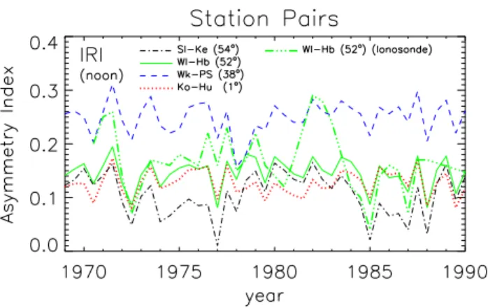
more slowly. The data points in his Fig. 3 are averages over latitude zones. Our Fig. 3 displays the solar cycle
be-Fig. 3. Variation of the annual asymmetry in peak electron density
at noon for four station pairs over two solar cycles, computed from ionosonde data.
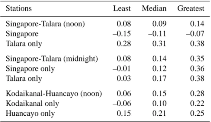
Table 2. Asymmetry index in ionosonde N mF2 for
Singapore-Talara (near geographic equator) and Kodaikanal-Huancayo (near geomagnetic equator).
Stations Least Median Greatest Singapore-Talara (noon) 0.08 0.09 0.14 Singapore –0.15 –0.11 –0.07 Talara only 0.28 0.31 0.38 Singapore-Talara (midnight) 0.08 0.14 0.35 Singapore only –0.01 0.12 0.36 Talara only 0.03 0.17 0.38 Kodaikanal-Huancayo (noon) 0.06 0.15 0.28 Kodaikanal only –0.06 0.10 0.22 Huancayo only 0.15 0.21 0.25
haviour in more detail, showing noon AI for four represen-tative pairs, computed from January and July monthly means of NmF2 over nearly two solar cycles. Each January point is computed from that January’s data, and from the mean of the preceding and following July. Likewise, each July point is computed from that July’s data, and from the mean of the pre-ceding and following January. This smoothes out the erratic values of AI that would otherwise be obtained when solar activity changes markedly in six months, as happens particu-larly at the start of solar cycles in 1977/1978 and 1987/1988. Figure 4 is similar, but is based on values of NmF2 taken from the International Reference Ionosphere, IRI-2000. However, because of the limitations of IRI, we should probably put more trust in the actual ionosonde data.
In Fig. 3, AI appears on the whole to be greater at solar maximum than at solar minimum, contrary to Yonezawa’s findings, though, as it applies to only some of the particular cases listed in Table 2, we do not regard this as a firm con-clusion. AI is greatest at lower mid-latitudes around 30◦,
Fig. 4. Variation of the annual asymmetry in peak electron density
at noon for four station pairs over two solar cycles, computed from the International Reference Ionosphere.
decreasing towards higher and lower latitudes. Except for the pair Slough-Kerguelen, for which AI sometimes drops to zero, AI is always positive and sometimes as large as 0.3, corresponding to a January/July ratio of 1.8 in (north + south)
NmF2. The results from IRI (Fig. 4) show little coherence
and do not agree well with the ionosonde results (which may say more about the IRI than about the ionosphere!).
We conclude from all these results that (i) the January/July asymmetry is real; (ii) it occurs both at noon and at midnight; (iii) it cannot reasonably be regarded as an accident of how stations are paired; (iv) it is much greater than the value 0.035 expected from the variation of Sun-Earth distance alone, and (v) on average it is greater at solar maximum than solar min-imum. We have not looked for any effect of geomagnetic activity on AI, which could only be established by a much more extensive analysis and would be difficult to separate from a solar cycle variation.
2.4 Equatorial stations
Low latitudes provide an interesting test of the characteris-tics of the annual asymmetry, because winter/summer vari-ations are weak or absent (though the semiannual varia-tion is strong). Both magnetic and geographic equators are of possible interest. For the former, we have Yonezawa’s pair Kodaikanal-Huancayo; for the latter, we use the pair Singapore-Talara; both pairs embrace Asian and American sectors. The available data sequences of NmF2 are 1957– 1965 for Singapore-Talara and 1969–1986 for Kodaikanal-Huancayo, though the midnight data are limited, espe-cially at the magnetic equator where the night F2-layer is highly structured and the critical frequency may not be well-determined.
In the special case of the equator, one can in principle determine an “annual asymmetry” with data from one sta-tion only. Accordingly, for each pair we have computed AI for the Asian station alone; for the American station alone;
and for both together (which of course is necessary for non-equatorial stations). Table 2 shows the least, median and greatest values of AI , to illustrate the considerable year-to-year scatter. We see that the American stations contribute more than the Asian stations to the combined AI ; indeed, the mean daytime AI for Singapore alone is negative.
These results suggest that in equatorial latitudes the an-nual asymmetry is quite strong in the American sector, but weak and possibly even reversed in the Asian sector. There is no very consistent pattern as to when the greatest and least values of AI occur, but generally speaking, the greatest val-ues of AI tend to occur near solar minimum, the smallest near solar maximum. The results for paired stations are more consistent than those for single stations, which may contain a seasonal effect.
Electron densities in the low-latitude topside ionosphere, measured at 600 km height by the Hinotori satellite (inclina-tion 31◦), were analysed by Su et al. (1998). They found a very large annual asymmetry of around 100% by day and 30% at night. Using the Sheffield University Plasmas-phere IonosPlasmas-phere Model (SUPIM), they suggest that annual changes in the transequatorial neutral winds are largely re-sponsible, together with changes of neutral composition. We discuss that in Sect. 3.1.
2.5 Results for total electron content
Does the annual asymmetry in NmF2 exist also in TEC (the total electron content in a vertical column through the ionosphere)? Titheridge and Buonsanto (1983) measured TEC using beacon satellites, at four stations that form two good pairs, Stanford-Auckland and Honolulu-Rarotonga, in years around the low solar maximum of 1969/1970 (mean
F10.7≈150), and related their findings to changes in
neu-tral composition. The results from these pairs are shown in Table 1 marked with small superscript “T”, and are consis-tent with equivalent ionosonde values. Note that Maui and Honolulu are so close together that both are designated “N” in the table. In pairs “F” and “G”, the northern sites are close together, but the southern ones are far apart in longi-tude, though equivalent in geographic and magnetic latitude. Titheridge and Buonsanto (1983) gave their results in terms of the mean, annual and semiannual Fourier compo-nents for day (10:00–16:00 LT) and night (22:00–02:00 LT). From these, we derived the annual asymmetry for each pair in two ways; first, by taking the annual/mean ratio from the sum of the Fourier terms for the north and south station (the results being shown in Table 1), and also by evaluating the January and July values from the Fourier series and apply-ing Eq. (3), with very similar results. For comparison, Ta-ble 2 shows also the asymmetry index for NmF2 of ionosonde pairs Akita-Townsville (roughly comparable with Stanford-Auckland) and Maui-Rarotonga (very nearly the same as Honolulu-Rarotonga), which agree quite well with those for TEC. The widespread existence of the annual asymmetry in
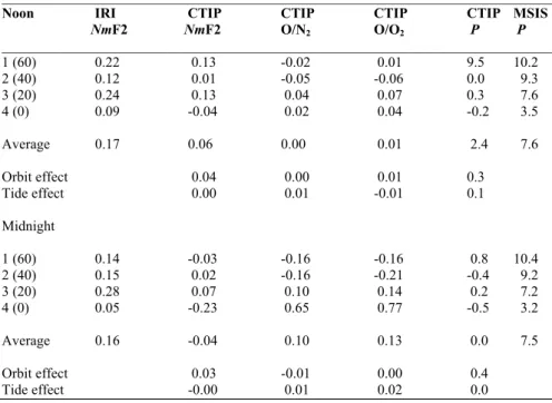
Table 3. Annual asymmetry for pairs of points at 162W, at magnetic latitudes 60, 40, 20 and 0. CTIP values include varying Sun Earth
distance. Neutral composition is computed at a fixed pressure-level. For further details see text. The only ionosonde comparison is with Maui/Rarotonga near pair 3, namely 0.36 for noon, 0.25 for midnight. Orbit effect is the difference (actual Sun-Earth distance – 1 AU). Tide effect is the difference (With tides) – (Without tides).
_________________________________________________________________________________
Noon IRI CTIP CTIP CTIP CTIP MSIS
NmF2 NmF2 O/N2 O/O2 P P _________________________________________________________________________________ 1 (60) 0.22 0.13 -0.02 0.01 9.5 10.2 2 (40) 0.12 0.01 -0.05 -0.06 0.0 9.3 3 (20) 0.24 0.13 0.04 0.07 0.3 7.6 4 (0) 0.09 -0.04 0.02 0.04 -0.2 3.5 Average 0.17 0.06 0.00 0.01 2.4 7.6 Orbit effect 0.04 0.00 0.01 0.3 Tide effect 0.00 0.01 -0.01 0.1 Midnight 1 (60) 0.14 -0.03 -0.16 -0.16 0.8 10.4 2 (40) 0.15 0.02 -0.16 -0.21 -0.4 9.2 3 (20) 0.28 0.07 0.10 0.14 0.2 7.2 4 (0) 0.05 -0.23 0.65 0.77 -0.5 3.2 Average 0.16 -0.04 0.10 0.13 0.0 7.5 Orbit effect 0.03 -0.01 0.00 0.4 Tide effect -0.00 0.01 0.02 0.0
TEC has been confirmed by a new study of global data by Mendillo et al. (2005), with AI averaging 0.15 over latitudes 0◦–65◦. We conclude that the annual asymmetry in NmF2 is
not simply due to vertical redistribution of ionization.
3 Neutral thermosphere
3.1 The MSIS model
Since it is widely accepted that F2-layer electron density is closely related to the ambient neutral O/N2ratio, we now
dis-cuss the experimental data on that ratio, both from the global empirical MSIS model of the neutral thermosphere and from the AE-C dataset, which was among the sources used to con-struct MSIS. We consider computational results on the O/N2
ratio and NmF2 in Sect. 4.
The MSIS-86 (mass spectrometer/incoherent scatter) model (Hedin, 1987) is constructed from a variety of exper-imental data, obtained from instruments aboard rocket and satellites and indirectly from measurements of the ionized gas by ground-based incoherent scatter radars. Being based on actual data, MSIS naturally includes any effect of Sun-Earth distance. A great deal of averaging and smoothing, which would affect results at particular places, is used in con-structing MSIS from the experimental data. This tends to smooth out latitude variations and features such as the peaks
of O/N2ratio at high winter latitudes (60◦–75◦) that are seen
in unsmoothed data and simulations of the CTIP model. The ratios (in particular O/O2) are subject to the serious
difficul-ties of measuring this ratio by satellite-borne instruments. The O/N2 ratio is very height-dependent, so we
exam-ine a parameter related to composition that has the great advantage of being height-independent provided the atmo-sphere is diffusively separated, with each major constituent having its own scale height, as is accepted to be the case at F2-layer heights. This is the P -parameter (Rishbeth and M¨uller-Wodarg, 1999) given by
P = 28 ln [O]−16 ln [N2] +12 ln T (5)
where square brackets indicate gas concentration and T is temperature. P is especially useful for analyzing satellite data. Roughly speaking, an increase of 1 unit in P corre-sponds to an increase of about 5.5% in O/N2 ratio. As P
is logarithmic, Eq. (3) cannot be used to define a meaning-ful asymmetry. Instead, we specify the annual asymmetry in composition for a station pair by differences instead of ratios, thus:
AI (P ) =
(P (North) + P (South))Jan−(P (North) + P (South))July(6)
The annual asymmetry in P , as given by MSIS, is mostly due to composition rather than temperature. The small an-nual variation in exospheric temperature, about ±10 K or
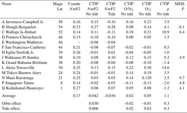
Table 4. Noon annual asymmetry at pairs of stations for moderate solar activity (F10.7∼140). Ionosonde values are taken from Table 1 (and
are averaged for the three pairs for which Table 1 values are at 100 and 180). CTIP values include varying Sun Earth distance. Neutral composition is computed at a fixed pressure-level. Orbit effect and tide effect as in Table 3. See text for further details.
Noon Magn I’sonde CTIP CTIP CTIP CTIP CTIP MSIS Lat N mF2 N mF2 N mF2 O/N2 O/2 p P
No tide Tide No tide No tide No tide A Inverness-Campbell Is 58 0.13 0.04 0.00 0.06 0.08 4.1 B Slough-Kerguelen 54 0.08 0.01 -0.02 –0.07 –0.10 –5.4 -0.6 C Wallops Is-Hobart 52 0.21 –0.06 –0.07 –0.23 –0.30 –11.0 6.5 D Poitiers-Christchurch 46 0.15 –0.01 –0.01 –0.04 –0.04 0.6 E Washington-Watheroo 46 0.15 0.04 0.05 0.01 0.03 2.7 F San Francisco-Canberra 44 0.18 –0.01 –0.01 –0.01 –0.00 0.8 H Eglin-Norfolk Is 39 0.34 0.02 0.03 –0.01 –0.00 0.9 J Wakkanai-Pt Stanley 38 0.21 0.11 0.02 0.12 0.17 9.9 5.0 K Grand Bahama-Brisbane 38 0.19 0.00 0.01 –0.05 –0.05 1.6 L Akita-Townsville 30 0.31 0.13 0.14 0.18 0.25 15.4 M Tokyo-Buenos Aires 24 0.27 0.08 0.07 0.03 0.04 3.9 N Maui-Rarotonga 21 0.36 0.08 0.09 0.07 0.10 2.4 9.6 P Singapore-Talara 8 0.09 –0.00 –0.01 –0.17 –0.21 –1.9 4.8 Q Kodaikanal-Huancayo 1 0.15 –0.07 –0.06 0.04 0.07 –1.0 5.6 Average 0.20 0.026 0.016 –0.01 0.00 1.4 Orbit effect 0.046 0.00 0.01 0.3 Tide effect –0.010 0.00 0.00 0.3
±0.8% with maximum in January, contributes <1 unit to AI(P ) which is too small to matter. This applies also to the AE-C data (Sect. 3.2).
The last column of Table 3 gives AI (P ) from MSIS for four pairs of points, 1–4, along the 162◦W meridian (see Sect. 4.3), while the last columns of Tables 4 and 5 give
AI (P ) for six station pairs covering a wide range of
lati-tude. Comparing the values of AI (P ) with AI of the ob-served NmF2 (as computed from the IRI data in Table 3 and the ionosonde data in Tables 4 and 5), we find that the asym-metry of NmF2 usually goes with an asymasym-metry in P that is of the right order to account for the asymmetry in NmF2 (Slough-Kerguelen is an exception, but may well be influ-enced by Kerguelen’s sub-auroral location, where the MSIS model may not be reliable). In every case, except Wakkanai-Port Stanley, MSIS gives an algebraically greater asymmetry than CTIP, though the tabulated asymmetries in P and O/N2
ratio do not correspond very closely. This may be because
P is very nearly height-independent, while the O/N2ratio is
derived on a fixed pressure-level near the F2 peak and (be-ing so rapidly height-vary(be-ing) can differ appreciably from the O/N2ratio actually at the peak. For that reason, the
sea-sonal composition differences at 600 km height, derived by Su et al. (1998) from the SUPIM computational model, do not reliably represent the composition at the F2-peak.
3.2 AE-C evidence for an annual variation in composition The AE-C data were obtained from the Neutral Atmosphere Temperature Experiment, NATE (Spencer et al., 1973) at al-titudes between 200 km and 450 km, acquired during 1975-1978 when the monthly mean solar 10.7 cm flux was in the range 70–100 units. This dataset was used by Rishbeth et al. (2004) to investigate seasonal variations. The data were taken at all local times, but mostly daytime (09:00– 15:00 LT), though the variation of composition does not ap-pear to vary much with local time.
We computed P for quiet magnetic conditions (Kp≤3),
and also for disturbed conditions (Kp>3) for which the
AE-C data are rather sparse. For the station pairs given in Table 4,
AI (P ) as given by Eq. (6) was positive for 8 stations, with
average value 5±6, for Kp≤3; for Kp>3 it was positive for
all 11 stations, with average 8±6. These averages respec-tively correspond to about 27% and 44% in O/N2ratio, with
no discernible trend with latitude. Despite the rather large scatter between stations, this is experimental evidence that the annual asymmetry does exist in neutral composition, and is roughly sufficient to account for the annual asymmetry in
NmF2. This supports the conclusions drawn from MSIS in
Sect. 3.1.
The AE-C results for north-south pairs of points along the 162◦W meridian, however, are rather different. For these, AI (P ) given by Eq. (6) is positive at latitudes 40–67◦
Table 5. Midnight annual asymmetry at pairs of stations for moderate solar activity (F10.7∼140). Ionosonde values are taken from Table 1
(and are averaged for the three pairs for which Table 1 values are at 100 and 180). CTIP values include varying Sun Earth distance. Neutral composition is computed at a fixed pressure- level. Orbit effect and tide effect as in Table 3. See text for further details.
Noon Magn I’sonde CTIP CTIP CTIP CTIP CTIP MSIS Lat N mF2 N mF2 N mF2 O/N2 O/2 p P
No tide Tide No tide No tide No tide A Inverness-Campbell Is 58 0.16 0.15 -0.16 0.16 0.23 3.5 B Slough-Kerguelen 54 -0.23 0.27 -0.28 0.08 0.14 4.1 -0.1 C Wallops Is-Hobart 52 0.14 0.11 -0.11 0.18 0.21 10.9 6.4 D Poitiers-Christchurch 46 0.15 –0.10 –0.10 0.00 0.05 1.5 E Washington-Watheroo 46 – –0.06 –0.04 F San Francisco-Canberra 44 0.21 –0.08 –0.07 –0.02 –0.01 0.5 H Eglin-Norfolk Is 39 0.26 –0.01 0.01 –0.04 –0.05 1.0 J Wakkanai-Pt Stanley 38 0.19 0.09 0.10 0.12 0.15 9.2 4.9 K Grand Bahama-Brisbane 38 0.20 –0.08 –0.06 –0.08 –0.10 –1.4 L Akita-Townsville 30 0.25 0.13 0.15 0.22 0.30 14.6 M Tokyo-Buenos Aires 24 0.24 –0.01 –0.01 0.14 0.19 3.5 N Maui-Rarotonga 21 0.25 0.03 0.03 0.14 0.120 2.5 9.7 P Singapore-Talara 8 0.14 –0.02 –0.03 –0.11 –0.13 –2.0 4.8 Q Kodaikanal-Huancayo 1 0.27 0.06 0.07 0.05 0.08 –1.2 4.1 Average 0.17 –0.042 –0.036 0.02 0.05 1.1 Orbit effect 0.030 –0.02 –0.01 0.3 Tide effect 0.006 0.02 0.03 0.3
but negative at lower latitudes. Furthermore, Mendillo et al. (2005), using global data from only two days in July 2002 and January 2003, found that the O/N2ratio derived from the
GUVI experiment on the TIMED satellite (Christensen et al., 2003), shows a smaller asymmetry of 0.06, while the NRL MSIS thermospheric model has an even smaller asymmetry of 0.03. We cannot expect complete consistency from every sample of data. It is interesting that in Figs. 5c, d, CTIP fol-lows MSIS fairly well in O/N2ratio for latitudes below 30◦
but poorly at higher latitudes.
4 Computational results
4.1 The CTIP model and simulations
We use the Coupled Thermosphere-Ionosphere-Plasma-sphere (CTIP) model described by Fuller-Rowell et al. (1996) and Millward et al. (1996), much as used by Zou et al. (2000) but with improved vertical resolution of1/
2scale
height, instead of one scale height as previously. The finer vertical resolution allows us to resolve tidal oscillations far better than before. There are now 31 pressure-levels, start-ing from the base of the thermosphere at height h=80 km at which the atmospheric pressure is p0=1.04 Pa. In most
runs we included the annual variation of Sun-Earth distance, which Zou et al. (2000) neglected. The program computes the parameters of the neutral air and ionized plasma with a
1-min time step on a latitude/longitude grid (2◦×18◦). The photochemistry does not include nitric oxide chemistry or the effects of vibrationally excited species. Some runs include tidal forcing at the lower boundary to account for dynamical coupling to the lower and middle atmosphere.
We assume a moderate level of solar activity, F10.7=100
(or F10.7=180 in some runs) and fairly quiet magnetic
condi-tions, Ap=9. Runs were made for the dates 4 January (Earth’s perihelion) and 4 July (Earth’s aphelion), in both cases for fixed Sun-Earth distance (1 astronomical unit, AU) and vary-ing Sun-Earth distance (0.983 AU for January, 1.017 AU for July). As the CTIP routines assume that the solar radiation fluxes are proportional to F10.7, we take the ionizing EUV
and X-radiations to be proportional to F10.7, which can only
be a rough guide but has no real effect on our conclusions. We allow for the inverse-square dependence of incident flux on Sun-Earth distance by setting F10.7 as 103.4 in January
and 96.7 in July. At noon, the model is not far from steady state.
At low latitudes our version of CTIP does not compute the dynamo electric fields self-consistently, but uses the empir-ical field model by Richmond et al. (1980). We would not expect the fields to make much difference (except perhaps during magnetic storms or at night in the equatorial zone), either to NmF2 or to neutral composition. Indeed, previ-ous computations with CTIP (Rishbeth and M¨uller-Wodarg, 1999) show no sign of any such equatorial effect. At high
Fig. 5. Latitude variations at longitude162◦W Above: Asymmetry index of NmF2 at noon and midnight. Dotted curves, CTIP, no meso-spheric tides, Sun-Earth distance fixed at 1 AU. Solid curves: CTIP including mesomeso-spheric tides, adjusted for Sun-Earth distance. Below: Asymmetry index of neutral O/N2ratio at noon and midnight. Dotted curves, CTIP, no mesospheric tides, with Sun-Earth distance fixed at 1 AU. Solid curves: CTIP adjusted for Sun-Earth distance, including mesospheric tides. Dashed curves: Mass Spectrometer Incoherent Scatter Model (MSIS). In all CTIP cases, the values for “no tide”, adjusted Sun-Earth distance’ (not shown) are about 0.03 higher than the 1 AU values.
latitudes we assume the convection field parameterized by Foster et al. (1986) and the auroral precipitation pattern from NOAA/TIROS satellites parameterized by Fuller-Rowell and Evans (1987).
In addition to the solar and magnetospheric forcing of the thermosphere/ionosphere system in CTIP, in some runs we include at the lower boundary the effects of tides propagat-ing upward from the lower and middle atmosphere. As de-scribed by M¨uller-Wodarg et al. (2001), the global diurnal and semidiurnal tides are implemented as perturbations of the height of the lower boundary pressure level and the hori-zontal winds and temperatures at that level. We assume west-ward propagating solar tides only and express their
latitudi-nal structure using Hough functions, in accordance with the standard theory described by Chapman and Lindzen (1970). The external input to CTIP are the amplitudes and phases for the Hough modes, the diurnal (1,1) mode and semidiurnal (2,2), (2,3), (2,4) and (2,5) modes, which describe a global profile of tidal oscillations at the bottom boundary level. Since we use propagating Hough modes only, tidal ampli-tudes in our simulations decrease towards the poles. The real atmosphere also includes considerable tidal waves at high latitudes which are described by vertically non-propagating Hough modes, but we ignore those in our study. The effects of including tides are discussed further in Sect. 5.
4.2 Orbit effect: the influence of varying Sun-Earth dis-tance on CTIP results
The annual variation of Sun-Earth distance is the most obvi-ous first cause of the annual asymmetry. We computed how much the orbital variation increases AI , both at noon and at midnight, for four pairs of points on the 162◦W meridian (see Sect. 4.3) and for the station pairs listed in Table 1. The results are shown as “Orbit effect” in Tables 3–5 and, as it varies so little between pairs, we just show the averages at the foot of each column.
On average the “orbit effect” contributes about 0.03 to the asymmetry of NmF2, just as expected. In neutral composi-tion the orbit effect is small and patchy (usually positive), but it is always greater for the O/O2than for the O/N2ratio. We
return to this last point in Sect. 4.5.
4.3 CTIP results for NmF2 and composition on the 162◦W meridian
We now study the annual asymmetry, computed as in Eq. (3), along the 162◦W meridian in the Pacific sector. This is one
of the 18◦longitude steps in the CTIP model, and is near the longitude where the geographic and magnetic equators cross so the geographic and magnetic latitudes are nearly equal. This meridian is remote from both North and South magnetic poles and about as far from auroral effects as it is possible to get, so geomagnetic effects should be minimized.
For comparison, we take NmF2 from the International Reference Ionosphere 2000 (IRI) (Bilitza, 2001). The only ionosonde pairs anywhere near this longitude are Maui and Rarotonga. To use the IRI, we found two January and two July quiet days in 1968 with similar conditions, computed
AI for the four pairings of these days (which varied little
among themselves), and averaged these values.
Table 3 shows the CTIP and IRI values of AI for three north-south pairs of points (1–3) and for a single point (4) for the special case of the magnetic equator at 2◦S. Pair 1 may be influenced by auroral effects, which may not be well modelled by CTIP or IRI. Values of AI for Pair 3 are simi-lar to those for Maui-Rarotonga (Sect. 4.4), which in global terms are not far away. As an experiment, we tried us-ing north-south pairs symmetric about the geographic equa-tor, instead of pairs in magnetic latitude. In general the geographically symmetric pairs have slightly larger values of AI , by about 0.03, than the magnetically symmetrical pairs, just as expected if the F2-layer structure is magneti-cally controlled. Table 3 also shows that the asymmetry in
P -parameter (Eq. 6), derived from MSIS, is much stronger
than in the CTIP results.
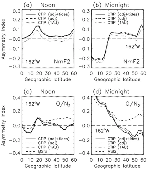
Panels (a, b) of Fig. 5 show the latitude variation of AI at longitude 162◦W, for noon and midnight NmF2, for three cases of CTIP: fixed Sun-Earth distance and no imposed tides (dotted line), varying Sun-Earth distance without imposed tides (dashed-dotted line) and varying Sun-Earth distance
with imposed semidiurnal tides (solid lines; see description in Sect. 5).
Panels (c, d) of Fig. 5 show how the asymmetry in the O/N2ratio varies with latitude. Again, the orbit effect is seen
to be small (and again the effect of tides is too small to be shown). Below 15–20◦the asymmetry in O/N2ratio (similar
for MSIS and for CTIP) varies quite sharply with latitude, and differently at noon and at midnight.
4.4 CTIP results for pairs of stations
Tables 4–5 show the asymmetries from CTIP computations for the pairs of points listed in Table 1. The station coordi-nates and ionosonde values of NmF2 are as in Table 1 (values for the Zou et al. pairs, Slough-Kerguelen, Wallops Island-Hobart and Wakkanai-Port Stanley are averages of F10.7=100
and 180), and CTIP and MSIS values assume F10.7=100. The
AI for O/N2 and O/O2composition ratios are computed as
in Eq. (3), at a fixed pressure-level near the daytime F2 peak. The average tide effect and orbit effect, at the foot of the ap-propriate columns, have been explained in Sects. 4.1 and 4.2. The overall impression from Tables 4 and 5 is that, both at noon and midnight, the asymmetry given by CTIP is numer-ically smaller than in the ionosonde data. This is the heart of the puzzle! Much the same applies to the asymmetry in
P given by CTIP, compared to that given by MSIS, in every
case except Wakkanai-Port Stanley. Although asymmetry in ionosonde NmF2 usually goes with asymmetry in MSIS P , the asymmetries in CTIP NmF2 and P seem only loosely re-lated, though we think the link is real.
As found in the ionosonde data (Sect. 2.3), at latitudes above about 45◦ the annual asymmetry in CTIP NmF2 is
closely connected to the seasonal (summer/winter) variation, which varies considerably from place to place. We made ex-periments in which one station of a pair was changed, and found that the re-computed AI depends on whether the sta-tions involved are in or out of a zone of large winter NmF2. This may explain why the Wallops Island-Hobart pair stands out in the CTIP simulations.
According to CTIP, the globally averaged O/O2ratio
in-creases from July to January by about 18% for varying Sun-Earth distance, but only 11% for fixed Sun-Sun-Earth distance. For the O/N2 ratio the corresponding figures are 10% and
7%.
4.5 The F2-layer loss coefficient and Buonsanto’s hypoth-esis
Buonsanto’s hypothesis about O2 dissociation involves
F-layer photochemistry. In the standard theory of the daytime F2 peak, photoionization (rate q), which depends mainly on the atomic oxygen concentration [O], approxi-mately balances photochemical loss. The loss coefficient β depends on the molecular nitrogen and oxygen concentra-tions, [N2] and [O2]. Neglecting transport processes (which
only become really dominant at heights above the F2 peak, though they control where the peak forms), the peak electron density is approximately given by the steady-state formula
N mF2 ≈ q/β ≈ I∞[O]/(k′[O2] +k′′[N2]) (7)
where k′, k′′ are the relevant rate coefficients and the ion-ization rate I∞ is proportional to the flux of solar ionizing
radiation and a weighted mean of ionization cross-sections for the neutral constituents. Although N2is more abundant
than O2by a factor of 10–20, the rate coefficients are such
that k′exceeds k′′by a similar factor (except when the N 2is
vibrationally excited and k′′is enhanced, which is not
gener-ally thought to be the case in quiet geomagnetic conditions at mid-latitudes). Thus both the O2and N2terms are likely
to be important in Eq. (7) and, as solar radiation dissociates O2much more strongly than N2, variations of Sun-Earth
dis-tance affects the O/O2ratio more than the O/N2ratio (though
the latter is affected by the change in O concentration caused by dissociation of O2). We therefore wish to see how much
the summer/winter change of atomic/molecular ratio is mod-ified by the extra change in O2dissociation due to changing
Sun-Earth distance.
In almost every case we computed with CTIP (Tables 3–5), we found the annual asymmetry is in-deed greater in O/O2than in O/N2, but only by about 0.02
on average (and about the same is found in MSIS). This difference is much too small to affect the conclusion that CTIP does not reproduce the observed asymmetries. So can we explain the annual asymmetry of NmF2 in terms of the O/O2ratio, as suggested by Buonsanto?
Our answer is “no, but it helps”. With the exceptions of the pairs Inverness-Campbell Island and Slough-Kerguelen (of which the southern stations are sub-auroral) and Akita-Townsville, the asymmetry even in the O/O2ratio is too small
to correspond to the ionosonde observations.
Buonsanto’s hypothesis would work best if the O2 loss
process dominates. So, as a further and probably decisive test, we did a computing experiment by supposing that k′is so much greater than k′′that only the O2loss process matters.
To that end, we ran CTIP with the N2loss process disabled,
while doubling the rate coefficient k′of the O2loss process
to keep the mean electron density roughly the same, in order that other factors in CTIP that depend on the ionization, such as thermal processes, would be more-or-less unchanged. We did the calculations for a fixed pressure-level near the mid-latitude F2 peak, rather than at the peak, but that should make little difference to the conclusions.
We found that our hypothetical assumption of “loss via O2only” increases the asymmetry AI only by about 0.01,
as compared to that with O2and N2loss processes together.
This increase is barely noticeable, so we have to abandon Buonsanto’s hypothesis, ingenious as it is, as an explanation of the F2-layer annual asymmetry. As a further detail, our computing experiment made little change to NmF2, which
implies that the N2and O2loss processes are of similar
im-portance at the F2 peak.
5 Thermospheric mixing by waves
In the following we investigate the question of F-region cou-pling to the neutral atmosphere via composition changes and thereby investigate how far the observed January/July asym-metry in NmF2 could be generated by the neutral atmosphere. In order for the F2-layer January/July asymmetry to be linked to processes in the neutral atmosphere, the asymmetry would need to be present also in the thermosphere, in particular the O/N2or O/O2ratios, both of which correlate with the
elec-tron densities. In Sect. 3.1 we showed that a January/July asymmetry could indeed be found in neutral composition from the MSIS model. In the following we investigate what processes can cause this asymmetry in the neutral gases. In Sect. 4 we showed that the CTIP model does not generate the observed January/July asymmetry either in the ionosphere or thermosphere. In the simulation discussed there we ignored coupling to lower regions in the atmosphere, so now we focus on the question of whether coupling to the regions below the thermosphere could be responsible for the neutral gas asym-metry found in MSIS.
5.1 Tides and composition
Tides are global oscillations in the atmosphere which are generated either thermally (“solar tides”) or gravitationally (“lunar tides”, plus a minor solar component) and propagate horizontally and vertically in the atmosphere. Solar tides are generated through absorption of solar radiation, primar-ily by water in the troposphere or ozone in the stratosphere, whereas lunar tides are a result of the Moon’s gravitational pull on the atmosphere. In general, solar tides are dominant over lunar tides.
As tides or other waves propagate upward in the atmo-sphere, their amplitudes grow with height roughly as the inverse square root of the mass density. When amplitudes reach critical values, they cause convection and turbulence and other damping processes that become important and limit the further amplitude growth. At that point, some of the wave energy and momentum is deposited in the background atmo-sphere, affecting temperatures and winds. Thus momentum and energy originating in the lower atmosphere is transported to higher regions in the atmosphere by tides or other waves.
In the thermosphere, the main wave damping processes are viscosity and vertical thermal conduction. While many of the higher frequency waves dissipate or break in the middle atmosphere, global scale waves such as tides and planetary waves are commonly found in the lower thermosphere. Typ-ically, planetary waves and the diurnal tide dissipate be-low 100 km altitude, while the semidiurnal tides can reach 200 km. Tides can have periods of up to a day or fractions
thereof, the most prominent ones found in the lower ther-mosphere having periods of 24 h, 12 h and 8 h. Up to around 120 km, tides dominate the daily variability of thermospheric temperatures and winds.
Solar and lunar tides are also observed in the ionosphere, where they produce drift motions of the plasma. However, away from the special circumstances of the geomagnetic equatorial zone, these tidal drifts do not directly produce marked effects on NmF2. In the non-auroral ionosphere,
NmF2 is largely controlled by photochemistry and, as shown
in Eq. (7), is linked to the neutral O/O2and O/N2ratios. It is
through this link that tides may have their strongest effect on
NmF2, as explored in the following.
Akmaev and Shved (1980) first suggested an influence of the upward propagating diurnal tide on atomic oxygen den-sities in the thermosphere. The mechanism they proposed is associated with the fact that vertical displacement of atomic oxygen by the diurnal tide in the lower thermosphere en-hances the effective three-body recombination rate, reduc-ing the atomic oxygen densities and creatreduc-ing a more molec-ular atmosphere. Similar results were obtained by Forbes et al. (1993) and Fesen (1997), using the TIME-GCM model. Their results show that both the diurnal and semidiurnal so-lar tides reduce the abundances of atomic constituents in the thermosphere through the same process as originally pro-posed by Akmaev and Shved (1980). In addition, these calculations predict a decrease of electron densities in the F-region by up to 20% caused by diurnal and semidiurnal propagating tides originating from below the thermosphere. Fuller-Rowell (1998) proposed an alternative process, by which the seasonal inter-hemispheric flow leads to stronger mixing of the thermosphere at the solstices compared with equinoxes, leading to more effective diffusive separation of constituents at equinox and thus a less molecular atmosphere. This was proposed as a mechanism to explain semiannual variations in neutral densities, which also affect the iono-sphere.
What these studies have shown is (a) how dynamics can affect neutral composition in the thermosphere through the effect of mixing either by waves or by large scale inter-hemispheric circulation and (b) that this potentially affects ionospheric plasma densities through changes in the recom-bination rates for ions. What none of these studies have shown is whether these processes could explain the iono-spheric January/July asymmetry, and it is this question we attempt to explore in the following.
5.2 Model runs
In order to investigate the effects of tides on the January/July asymmetry, we ran CTIP for several cases which included tidal forcing at the lower boundary, implemented in the way described in Sect. 4.1, using the diurnal (1,1) Hough mode and semidiurnal (2,2), (2,3), (2,4) and (2,5) modes. We ran two cases of tidal forcing. Case 1 was run for 4 January and
4 July, assuming different tidal amplitudes, namely: January: (1,1) 100 m/12.0 h; (2,2) 355 m/3.8 h; (2,3) 84 m/13.3 h; (2,4) 76 m/5.4 h; (2,5) 118 m/4.4 h and July: (1,1) 200 m/12.0 h; (2,2) 266 m/4.0 h; (2,3) 56 m/3.1 h; (2,4) 52 m/10.1 h; (2,5) 87 m/10.7 h. On average, therefore, we reduced the semidi-urnal amplitudes by a factor of 1.4 in July in Case 1, while doubling the diurnal amplitude. This is consistent with the climatology by Forbes and Vial (1989), although we en-hanced the overall strength of tidal forcing in our model to strengthen the potential effect. Case 2 was run for 4 January and 4 July as well as for the March and September equinoxes, assuming for all months tidal amplitudes and phases of (1,1) 100 m/12.0 h; (2,2) 400 m/3.8 h; (2,3) 300 m/3.8 h; (2,4) 200 m/5.4 h; (2,5) 100 m/4.4 h. All tidal runs for January and July include the variation of Sun-Earth distance as described in Sect. 4.1 and differ from those simulations only with re-spect to tidal forcing.
5.3 Tidal effects on NmF2 computed from CTIP
Tables 3–5 summarize the results of our simulations with Case 1 tidal forcing, which indicate that tides have a small effect only on the strength of the January/July asymmetry both in neutral composition and NmF2. Since our tidal am-plitudes, based on the climatology by Forbes and Vial (1989), are assumed to differ between January and July by only a fac-tor of 1.4, we furthermore calculated the annual asymmetry indices for a tidal January and non-tidal July simulation (and vice versa), thus maximizing the difference in lower bound-ary forcing, but found very similar results irrespective of the tidal forcing. While we find a general difference between
NmF2 with and without tidal forcing, in agreement with
re-sults by Forbes et al. (1993) and Fesen (1997), we are un-able to enhance the January/July asymmetry with the tides. We find the tidal effect on composition to be in the same sense at all local times, which implies that the tidal effect is “rectified” with a time constant greater than 24 h. We may conclude that the tides have a “stirring-up” effect on ther-mospheric composition, which acts to increase the molec-ular/atomic ratio in the thermosphere and decrease electron densities, smoothing out local time variations, as expected since thermospheric composition takes about 20 days to set-tle (Rishbeth et al., 2000a). This tends to confirm that the effects on NmF2 are not due directly to the oscillatory drifts in the F2-layer plasma, which have little net effect on the electron density at mid-latitudes.
The weak influence of tides in our simulations at first appears to contradict the findings by Forbes et al. (1993) so, to verify the consistency of CTIP with the TIGCM Model which they used, we carried out simulations for iden-tical seasonal and tidal conditions as they. We found the same decrease in F-region electron density and O/N2
ra-tio as they did, confirming that CTIP reproduces correctly the underlying physical processes and thereby validating our model. Since the January/July asymmetry assumes solstice
Fig. 6. Effect of mesospheric tides on values of asymmetry
in-dex, as percentage of non-tide values. Above: Solstices, Below: Equinoxes. Full curves: Peak electron density. Dashed curves: Neutral O/N2ratio at the height of the F2-peak. All curves are for
local noon.
and not equinox conditions, we will in the following examine whether seasonal conditions could affect the tidal influences on neutral and ion composition.
Figures 6 and 7 show results from our Case 2 simulations, which assumed the same tidal amplitudes at all seasons. Shown are the normalized changes (AItidal−AInon−tidal)/
AInon−tidal of the asymmetry index AI due to tidal
forc-ing in the model versus geographic latitude. Solid lines are changes of NmF2, dashed lines are those of O/N2taken at the
height of peak electron density hmF2. The upper panels show changes at January and July, the bottom panels are changes at the equinoxes. All values are shown along the 162◦W merid-ian to minimize effects due to the offset of the geographic and geomagnetic poles. Figure 6 shows values at local noon, Fig. 7 at local midnight. We see that noon changes of NmF2 in general shape correlate well with those of O/N2,
confirm-ing our expectation (see Sect. 4.5) from photochemical con-siderations, but at the same time some deviations between the dashed and solid curves are present which suggest the in-fluence of plasma transport. The correlation between NmF2 and O/N2 is less apparent on the nightside (Fig. 7), where
changes of O/N2 reach far greater values than on the
day-Fig. 7. As day-Fig. 6 for local midnight.
side, in particular at equinox, but those of NmF2 are fairly invariant. Nighttime NmF2 is more strongly controlled by transport.
The response of O/N2 at F2-layer altitudes to tidal
forc-ing strongly depends upon latitude, as does the structure of tides. At equatorial latitudes, where tidal forcing amplitudes are largest, we find an enhancement of O/N2at the solstices
(upper panels of Fig. 6), whereas towards high mid-latitudes (40◦–60◦) more complexity is apparent which suggests the influence of high latitude forcing (in particular through ion drag). We found the behaviour at E-region altitudes (not shown) to be far more uniform and symmetric with latitude and not to include those higher latitude features. Tides over-all appear to decrease O/N2on the dayside at some latitudes,
but we equally find regions where the value has increased with tidal forcing. So, the picture appears to be more com-plicated than the simple idea that mixing due to tides in-creases the abundance of molecular constituents and hence decrease O/N2. At local midnight (Fig. 7), large tidally
induced changes are apparent in O/N2, particularly at the
equinoxes, but that hardly affects NmF2 which is controlled primarily by transport processes.
Interesting differences are apparent between the responses at solstice (upper panels in Figs. 6 and 7) and equinox (lower panels). At equinox the response to tidal forcing is gener-ally stronger than at solstice, on average 10–15% as opposed
to 5–10%. This effect is even stronger at E-region altitudes (not shown). This result is interesting in that it shows that the way in which tides affect the thermosphere depends on the background circulation, which is different at equinox and solstice.
As outlined by Duncan (1969) and described by Rishbeth et al. (2000a), a summer-to-winter hemisphere circulation cell is present in the thermosphere at solstice, with average meridional wind velocities of around 25 m s−1. This in itself causes a departure of the gas distribution from diffusive equi-librium, as noted also by Fuller-Rowell (1998), and the effect of tides on composition at the solstices is hence reduced. At equinox, in contrast, the low-to mid-latitude thermosphere in the absence of tides is undisturbed overall and close to equi-librium distribution, so tidal disturbances generate an overall stronger response. The well-defined latitudinal responses in Figs. 6 and 7 show that the main effect on neutral composi-tion is via the effect of tides on the background circulacomposi-tion, altering the vertical velocities. Since this effect depends upon the magnitude of background (diurnally averaged) winds at a particular location, which themselves depend on latitude, we see pronounced latitudinal variations. So, the tidal effect on O/N2at F2-layer altitudes is not a general ‘stirring-up’ of
the atmosphere, but a more localized effect via the manner in which background horizontal and vertical winds are altered due to wave dissipation.
In principle, plasma transport along magnetic field lines due to neutral winds also affect the recombination rate of ions, and hence NmF2. However, we find tidal dissipa-tion primarily affects the zonal and vertical velocities and to less extent the meridional ones. Since we assumed west-ward propagating tides only, zonal winds generally experi-ence westward acceleration. This has little effect on plasma densities, except to some extent in the dawn and dusk sectors. In summary, we found daytime O/N2and NmF2 to respond
overall similarly to tidal forcing, but this response is strongly latitude dependent. At night, tidal changes to O/N2are more
pronounced, but those of NmF2 are similar to or smaller than daytime changes. The thermosphere appears to respond less strongly to tidal forcing at solstice than at equinox. This be-haviour helps us understand the weak effect that tides have on the January/July asymmetry: while locally there is an ef-fect, it is too weak to alter our results significantly from the non-tidal runs.
5.4 Waves not included in the computations
In our simulations we ignored non-propagating tides as well as planetary waves and gravity waves. By non-propagating tides we mean atmospheric tides that do not propagate in the vertical direction, but horizontally only. Their occurrence and effects on the atmosphere are therefore largely limited to the height region where they are excited. This is primarily in the troposphere and stratosphere, far below our region of interest, justifying our assumption.
Because of the coarse grid size in longitude, CTIP can-not represent the propagation of planetary waves. Although gravity waves of various periods are a well-known feature of the F2-layer, the mere passage of a gravity wave does not seem to have any lasting effect on the electron density. Again as with tides, the most important effect of gravity waves (so far as the present work is concerned) is likely to be enhanced mixing in the lower thermosphere. Their forc-ing is greatest in the Northern Hemisphere in winter, partly as a result of topography and partly because of seasonally varying zonal winds that modulate the upward propagation of gravity waves. Gravity waves (other than solar tides) are not included in the CTIP version used in this paper.
6 Are there annual variations in other ionospheric pa-rameters?
6.1 Height of F2 peak
In their study of semiannual variations of the F2 peak height
hmF2, Rishbeth et al. (2000b) also derived 12-month
compo-nents for sixteen stations, including three of the pairs listed in Table 1. The three northern stations of these pairs (Slough, Wakkanai, and Washington/Wallops Island) have maximum noon hmF2 in early summer (April–May), while the south-ern stations (Kerguelen, Port Stanley, and Mundaring (which replaced Watheroo)) have maximum hmF2 in late summer (January–February). Thus on average the annual asymme-try in hmF2 peaks around March equinox. The correspond-ing amplitudes are 10–20 km for the northern three stations, about 20 km for Kerguelen and Mundaring, and no less than 40 km for Stanley, where the large amplitude is attributed to the strong, seasonally varying meridional winds in the South Atlantic sector. As discussed in Sect. 7.5, the hemispheric imbalance in the winds may have implications for the annual asymmetry of NmF2.
6.2 E-layer electron density N mE
We have looked for an asymmetry in noon E-layer electron density for the “Zou et al. pairs” of stations, using Eq. (3) with N mE instead of NmF2. The E-layer data for the six stations contained many missing values, but nevertheless the annual asymmetry could be estimated, though not with high accuracy. Averaging over low and high solar activity (re-spectively F10.7=100 and 180), the computed values of AI
for N mE are 0.01 for Slough-Kerguelen, 0.035 for Wallops Island-Hobart, and 0.08 for Wakkanai-Port Stanley. With the square-law loss process in the E-layer, the expected asym-metry due to Sun-Earth distance is 0.017. We thus find no evidence of a consistent January/July asymmetry in E-layer electron density. We cannot look for evidence for any annual asymmetry in the F1-layer, because the ionosonde data are too sparse in winter to enable any valid study. Thus, as far as