Mixed finite element formulation in large deformation frictional contact problem

(1)

HAL Id: insu-00355357

https://hal-insu.archives-ouvertes.fr/insu-00355357

Submitted on 22 Jan 2009

HAL is a multi-disciplinary open access archive for the deposit and dissemination of sci-entific research documents, whether they are pub-lished or not. The documents may come from teaching and research institutions in France or abroad, or from public or private research centers.

L’archive ouverte pluridisciplinaire HAL, est destinée au dépôt et à la diffusion de documents scientifiques de niveau recherche, publiés ou non, émanant des établissements d’enseignement et de recherche français ou étrangers, des laboratoires publics ou privés.

Mixed finite element formulation in large deformation

frictional contact problem

Laurent Baillet, T. Sassi

To cite this version:

Laurent Baillet, T. Sassi. Mixed finite element formulation in large deformation frictional contact problem. Revue Européenne des Éléments Finis, HERMÈS / LAVOISIER, 2005, 14 (2-3), pp.287 à 304. �10.3166/reef.14.287-304�. �insu-00355357�

(2)

Revue européenne des éléments finis. Volume X – n° X/2002, pages 1 à X

deformation frictional contact problem

Laurent Baillet* — Taoufik Sassi**

* Laboratoire de Mécanique des Contacts et des Solides, CNRS-UMR 5514 INSA de Lyon, 69621 Villeurbanne Cedex, France

e-mail: laurent.baillet@insa-lyon.fr

** Laboratoire de Mathématiques Nicolas Oresme CNRS 6139 Université de Caen

Bd du Marechal Juin, 14032 CAEN Cedex e-mail sassi@math.unicaen.fr

ABSTRACT. This paper presents a mixed variational framework and numerical examples to

treat a bidimensional friction contact problem in large deformation. Two different contact algorithms with friction are developed using the 2D finite element code PLAST2.

The first contact algorithm is the classical node-on-segment, and the second one corresponds to an extension of the mortar element method to a unilateral contact problem with friction. In this last method, the discretized normal and tangential stresses on the contact surface are expressed by using either continuous piecewise linear or piecewise constant Lagrange multipliers in the saddle-point formulation. The two algorithms based on Lagrange multipliers method are developed and compared for linear and quadratic elements.

RÉSUMÉ. Une étude numérique de différentes méthodes d’éléments finis avec multiplicateurs

de Lagrange pour les problèmes de contact avec frottement de Coulomb en grand déplacement est menée dans cet article. Le problème de point-selle correspondant est approché par des éléments finis linéaires ou quadratiques. Les conditions de contact et de frottement discrétisées sont exprimées au sens faible (raccord de type intégral). Ces approches généralisent la méthode des éléments finis avec joints aux problèmes de contact frottants. La mise en oeuvre de ces techniques est réalisée dans la nouvelle version du code de calcul par éléments finis en deux dimensions PLAST2. Des comparaisons sont effectuées avec la méthode du raccord classique “noeuds-segments” initialement implantée dans PLAST2.

KEY WORDS: contact, mixed finite element, friction, dynamic explicit, mortar elements.

(3)

1. Introduction

In order to solve a contact problem with friction, it is necessary to possess numerical tools adapted to the strong non-linearity, the incompatibility of meshing on the contact zone and the evolutionary characteristics of the surfaces.

Methods used differ by their contact algorithm, their time integration scheme and the construction of the global contact matrices obtained from the writing of the non interpenetration condition. The solution to a contact problem is obtained using various methods such as the penalisation or the Lagrange multiplier methods (Chaudhary, 1986), (Kikuchi, 1988), (Wriggers, 1995), (Zhong, 1992), (Wriggers, 1990), (Rebel, 2002). Among these last methods one finds the gradient methods (Raous, 1992), (May, 1986), those of the increased Lagrangian or other mixed approaches (Klarbring, 1986), (Simo, 1992), (Alart, 1991).

For the resolution of a contact problem without friction using the Lagrange multipliers method, the construction of the global contact matrices used for the calculation of contact stresses is not unique. Usually, the classical node-on-segment strategy (local type approach) is used. The mortar element method initially presented for domain decomposition has been used for the resolution of a unilateral contact problem (Hild, 1998-2000-2002). The introduction of another Lagrange multiplier related to the tangential friction stress following a Coulomb or Tresca law has been presented by the researchers (McDevitt, 2000), (Baillet, 2003). McDevitt and Laursen have used the mortar element method in the case of small deformations, by using the penalisation method and for problems of non evolutionary contact surfaces.

In this paper, the contact treatment is based on the mortar-finite elements method (global type approach), it uses the Lagrange multiplier method and is developed for large deformation problems where the contact surface is evolutionary. These algorithms have been implemented and tested in the 2D finite element code PLAST2. PLAST2 includes large deformation and non linear material behavior. It is based on a Lagrangian-mesh Cauchy-stress formulation in conjunction with an explicit time integration scheme. The forward Lagrange multiplier method is used to treat the contact between deformable bodies.

The paper is organized as follows. First we introduce the equations modeling the Signorini problem with friction, continuous mixed variational formulation and contact algorithms are presented. Then several numerical simulations which include contact between deformable bodies are performed. Comparisons of the two contact algorithms, the choice of the discretized normal and tangential stresses and the choice of the element (linear Q1 or quadratic Q2) are carried out. The numerical examples illustrate the accuracy and robustness of the proposed mortar-finite element formulation for a contact problem with friction in large deformation.

(4)

2. Continuous problem and functional framework

One considers the deformation of two elastic bodies occupying, in the initial

configuration, two domains Ωj

, j=1,2. For j=1,2 the boundary Γj

of each solid is

the union of three non-overlapping parts j

c j g j u j=Γ ∪Γ ∪Γ

Γ . The displacement field

is known on j

u

Γ (one can suppose, for example, that the Ωj

solid is embedded in j

u

Γ ). The j

g

Γ boundary is submitted to a density of forces noted j 2 j 2

)) ( L (

g ∈ Ω .

Initially the two solids are in contact on the common part of their boundary

2 c 1 c c =Γ =Γ Γ . The Ωj body is submitted to j 2 j 2 )) ( L (

f ∈ Ω forces. The normal unit

outward vector on Ωj

is noted j

n as one designated by µ≥0 the friction

coefficient (supposed constant on Γc by simplification).

The Coulomb problem of contact with friction consists in finding the j

u displacements and the σ(uj)

stresses which verify the following equations and conditions , in ) u ( D ) u ( j = jε j Ωj σ [1] , in 0 f ) u ( divσ j + j = Ωj _[2] , on g n ) u ( j g j j j = Γ σ [3] , on 0 u j u j = Γ _[4] in which ε(uj)

represents the linearized strain tensor, j

D is the fourth order tensor satisfying the usual symmetry and ellipticity conditions in elasticity. Equations [1], [2], [3] and [4] respectively designate the behaviour relation, the equilibrium equation and the Neumann and Dirichlet condition.

To introduce the equations onto the Γc contact zone, the following notations are

adopted , )t u ( n ) u ( n ) u ( , u u u n ) n . u ( u j t j j n j j j t j n j t j j j j = + = + σ =σ +σ [5] where uj n and u j

t respectively represent the normal and tangential

displacements and (uj)

n

σ and (uj)

t

σ respectively designate the normal and tangential stresses where t is a unitary fixed tangent vector.

The equations modelling the unilateral contact on Γc become

. 0 ] u )[ u ( , 0 ) u ( , 0 ] u [ n ≤ σn ≤ σn n = [6]

The [u_n] notation represents the (u1.n1+u2.n2)

jump of the normal displacement through the Γc contact zone. The [6] conditions, expressing the

unilateral contact between the two bodies, describe respectively the non-penetration condition, the sign condition on the normal stress and the complementary condition.

(5)

The conditions of Coulomb’s friction on Γ_c are written       λσ − = ≥ λ ∃ ⇒ σ µ = σ = ⇒ σ µ < σ σ µ ≤ σ ). u ( ] u [ s.t. 0 ) u ( ) u ( , 0 ] u [ ) u ( ) u ( , ) u ( ) u ( t t n t t n t n t & & [7]

Here [u&t] represents the jump of the tangential velocity through Γc.

Remark: in this paper, we are interested in the discrete formulation with Lagrange multipliers of the friction. Then we restrict ourself to the displacement formulation of the friction and we replace [u&t] in [7] by [ut].

Let us consider K as the closed convex cone of admissible displacements which satisfies the conditions of non penetration

{

}

{

j

}

u 2 j 1 j j c n 2 1 2 1 on 0 v , )) ( H ( v V where on 0 ] v [ ; V V ) v , v ( v K Γ = Ω ∈ = Γ ≤ × ∈ = = . [8]

The variational formulation corresponding to problem [1]-[7], obtained by Duvaut and Lions (Duvaut, 1972) consists of finding u which verifies

K v , ) u v ( L ) u , u ( j ) v , u ( j u) -v u, ( a , K u∈ + − ≥ − ∀ ∈ [9] where

∫

Ω Ω ε ε = + = j j j j j 2 1 , d )) v ( : ) u ( D ( ) v u, ( a , v) u, ( a ) v u, ( a v) u, ( a [10]

∫

∑∫

∫

Γ = Ω Γ Γ σ µ = Γ + Ω = c t n 2 1 j j j u j j j j , d ] v [ ) u ( v) u, ( j , d v . g d v . f ) v ( L [11]

are defined for all u and v in Sobolev’s standard space 1 2

)) ( H

( Ω . The functional

(6)

3. Mixed variational formulation of the discrete problem

Let j

h

ℑ be a regular family of partitions of Ωj

into triangles (or quadrangles) κ

U

j h j . ℑ ∈ κ κ = Ω [12]

The discretisation parameter h on j

j Ω is given by κ ℑ ∈ κ =maxh h j h j [13]

where h denotes the diameter of the triangle (quadrangle) _κ κ. Let

) h , h max(

h= 1 2 . For any integer q≥0, the notation Pq(κ) denotes the space of the

polynomials with the global degree ≤q on κ. The finite element space used in Ωj

is then defined by

{

v (C( )) , ,v (P ( )) ,v 0

}

,q 1or 2, V j u j h 2 q j h j h 2 j j h j h = ∈ Ω ∀κ∈ℑ κ∈ κ _Γ= = [14]

and the approximation space of V becames 2

h 1 h h V V

V = × .

The contact zone Γc inherits two independent regular families of

monodimensional meshes. The set of nodes belonging to triangulation j

h ℑ are denoted

{

j

}

) h ( N j 1 ) h ( N j 1 j 0 j h = x <x <...<x <x ξ − . [15]

In order to express the constraints by using conveniently chosen Lagrange multipliers on the contact zone, we have to introduce first the space describing the degree of the polynomial approximation

{

v ,v V

}

W ( ) W ( ) ) ( W c j , 1 ht c j , 1 hn j h j h j c h c j , 1 h Γ = Γ ∈ = Γ × Γ

]

[

(

z ,z

)

,0 i N(h) W ( ) W ( ) P , ) ( W c j , 0 ht c j , 0 hn j 1 k j k 0 j 1 k z , j k z h h c j , 0 h _= Γ × Γ     ≤ ≤ ∈ µ µ = Γ +     + [16] where j 0 j 0 x z = , j ) h ( N j 1 ) h ( N x z + = and for k=1,...,N(h)-1, j k

z denotes the middle of segment

[

j

]

K j 1 k j 1 k x ,x T ₋ = ₋ .

(7)

The Lagrange multipliers associated to the normal and tangential stresses on the

Γc contact surface either belong to the space W( c) 1

h Γ consisting of continuous

piecewise linear functions either belong to the W ( c)

0

h Γ space consisting of constant

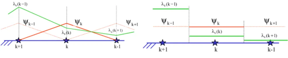
piecewise functions (figure 1).

k k+1 k-1 k ψ ψk+1 1 k− ψ ) 1 k ( h + λ ) k ( h λ ) 1 k ( h − λ Lagrange multipliers W ( c) 1 h Γ ∈ k k+1 k-1 k ψ ψk+1 1 k− ψ ) 1 k ( h − λ ) k ( h λ ) 1 k ( h + λ Lagrange multipliers W ( c) 0 h Γ ∈

Figure 1.Graphic representation of the two Lagrange multiplier spaces

Next, we introduce the convex cones associated to the normal and tangential stresses on the contact zone Γc. Let

1 ht 1 hn 1 h M M

M = × be the convex sets of continuous piecewise linear Lagrange multipliers

        Γ ≥ ψ Γ ∈ ψ ∀ ≥ Γ ψ µ Γ ∈ µ =

∫

Γ c h c 1 hn h c h h c 1 hn h 1 hn W ( ), d 0, W ( ) , 0on M

,

        Γ ∈ ψ ∀ Γ ψ ≤ Γ ψ µ Γ ∈ µ =

∫

Γ Γ ) ( W , d s d ), ( W M c 1 ht h c h h c h h c 1 ht h 1 ht

,

[17]

where sh is the given slip bound on Γc. We then consider the convex sets of

piecewise constant Lagrange multipliers denoted 0

ht 0 hn 0 h M M M = × and defined on c Γ as follows         Γ ≥ ψ Γ ∈ ψ ∀ ≥ Γ ψ µ Γ ∈ µ =

∫

Γ c h c 1 hn h c h h c 0 hn h 0 hn W ( ), d 0, W ( ) , 0on M

,

        Γ ∈ ψ ∀ Γ ψ ≤ Γ ψ µ Γ ∈ µ =

∫

Γ Γ ) ( W , d s d ), ( W M c 1 ht h c h h c h h c 0 ht h 0 ht

.

[18]

In order to solve the Coulomb’s frictional contact problem [9] with Lagrange multipliers method, we introduce the following intermediary problem with a given

(8)

, M M ) , ( , 0 d ] u )[ ( d ] u )[ ( , V v ), v ( L d ] v [ d ] v [ ) v , u ( a : that such M M V ) , , u ( Find ht hn ht hn c ht ht ht c hn hn hn h h h c ht ht c hn hn h h ht hn h ht hn h × ∈ ν ν ∀ ≤ Γ λ − ν + Γ λ − ν ∈ ∀ = Γ λ − Γ λ − × × ∈ λ λ

∫

Γ Γ Γ Γ [19] where 0 hn 1 hn hn M or M M = and 0 ht 1 ht ht M or M M = .

The discrete mixed problem P(sh) admits a unique solution (see (Haslinger,

1982)). It becomes then possible to define a map Φh as follows

hn h hn hn h s M M : λ → → Φ [20]

where (uh,λhn,λht) is the solution of P(sh). The introduction of this map allows the definition of a discrete solution of Coulomb’s frictional contact problem [9].

4. Matrix formulation of the global type approach

The matrix formulation of the mixed problem of two bodies Ω1

and Ω2

in contact is given by fixing h, the element lengths. One then has a discretization including N=N1+N2 nodes where N1 is the number of nodes belonging to Ω1. The N

basic functions of Vh are noted ϕi, i=1,…,N so that if u (u ,u ) 2 h 1 h h = we have

∑

+ = = ϕ = ϕ = N 1 1 N i i 2 h 2 1 N 1 i i 1 h 1 ) i ( u u and ) i ( u u

.

[21]

We designate by m the number of nodes (i=1,…m) on 1 c

Γ (slave surface) belonging to the Ω1

mesh and by n (i= N1+1,…N1+n+1) the number of nodes on

2 c

Γ (master surface) belonging to the Ω2

mesh. The discrete multipliers of the normal and tangential contact stresses are defined on 1

c Γ as follows

∑

= = ψ λ = λ ψ λ = λ m 1 k k ht ht m 1 k k hn hn (k) and (k)

,

[22]

where ψk are the m basic functions on 1 c

Γ at the k nodes. P(sh)

(9)

The first discrete formulation equation of the contact problem with friction on the Ω1

domain has the following matricial form

1 1 T 1 N 1 1 F 0 G G U K Λ=           −

,

[23] where 1

K designates the elastic rigidity matrix linked to Ω1

, 1

U designates the

vector whose components are the nodal values of 1

h

u and Λ=(ΛN,ΛT) the vector

of components λhn(k), λht(k) for k=1,…,m. The vector of exterior forces is noted

1

F whereas 1

T 1 N ,G

G are the coupling symmetrical matrices (of order m) between

multipliers and displacements. The coefficients of 1

T 1 NandG G matrices are respectively defined by . m j i, 1 , d t . a , m j i, 1 , d n . a j 1 c i 1 j , i j 1 c i 1 j , i ≤ ≤ Γ ψ ϕ = ≤ ≤ Γ ψ ϕ =

∫

Γ Γ [24]

Remark : for a fixed choice of all the multipliers, the 1 T 1 N andG

G matrices are identical and will be noted 1

T 1 N 1 G G

G = = . In the same manner, the system of unknown equations 2 U and Λ on Ω2 is written 2 1 , 2 T 1 , 2 N 2 2 F 0 G G U K Λ=           −

,

[25] 1 , 2 T 1 , 2 N 1 , 2 G G

G = = is a rectangular matrix of n lines and m columns whose coefficients are . m j 1 et 1 n N i N , d n . a j 1 1 2 c i 1 , 2 j , i =

∫

ϕ ψ Γ ≤ ≤ + + ≤ ≤ Γ [26]

(10)

      = Λ               −             2 1 1 , 2 1 2 1 2 1 F F 0 G 0 G U U K 0 0 K

.

[27]

The interest now is in the matricial writing of the contact and friction conditions

∫

Γ Γ ∈ ν ν ∀ ≤ Γ λ − ν + Γ λ − ν c h ht hn ht ht ht c hn hn hn )[u ]d ( )[u ]d 0, ( , ) M (

,

[28] with 1 ht 1 hn h M M M = × or 0 ht 0 hn h M M

M = × . Let U and N U be the vectors T

whose components are respectively the nodal values of [uhn] and [uht]. It can be

shown (Baillet, 2003) that the preceding inequation is written

           ≤ − + Λ = − + ⇒ Λ µ − < Λ Λ µ − ≤ Λ ≤ − + Λ ≤ − + ≤ Λ − − − − . 0 ) U ) G ( ) G ( U ( ) G ( , 0 ) U ) G ( ) G ( U ( ) ( ) G ( , ) ( ) G ( , 0 ) U ) G ( ) G ( U ( ) G ( , 0 ) U ) G ( ) G ( U ( , 0 ) G ( i 2 T t 1 , 2 1 1 1 T i T 1 i 2 T t 1 , 2 1 1 1 T i N i T 1 i N i T 1 i 2 N t 1 , 2 1 1 1 N i N 1 i 2 N t 1 , 2 1 1 1 N i N 1 [29]

4.1 Construction of the G1 and G2,1 matrices

In the case of the basic functions ψ_k on 1

c

Γ , continuous piecewise linear (P1) or

constant piecewise (P0) and for the Q1 finite elements, the construction of the

1

G and 2,1

G matrices is described in this paragraph. The 1

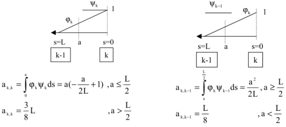
G matrix coefficients for

functions ψk of the P0 and P1 type are shown on figure 2 and 3 respectively.

The 2,1

G matrix is the matrix coupling the m slave nodes of the 1

c

Γ surface and

the n master nodes of the 2

c

Γ surface. To determine the expression of the

coefficients of this coupling matrix, in the case when the surfaces are not smooth (figure 4.a), it is necessary to proceed first of all to a projection of the interface nodes onto a curvilinear abscissa that is noted “s” (figure 4.b).

(11)

s=0 s=L a k k-1 1 k ψ k ϕ 2 L a , L 8 3 a 2 L a , ) 1 L 2 a ( a ds a k , k a 0 k k k , k > = ≤ + − = ψ ϕ =

_∫

s=0 s=L a k k-1 1 1 k− ψ k ϕ 2 L a , 8 L a 2 L a , L 2 a ds a 1 k , k 2 2 L a 1 k k 1 k , k < = ≥ = ψ ϕ = − − −

∫

Figure 2. Coefficient of 1

G for P0 shape functions ψk

s=0 s=L a k k-1 1 k ψ k ϕ ) 1 L a L 3 a ( a ds a ₂ 2 a 0 k k k , k =

∫

ϕ ψ = − + s=0 s=L a k k-1 1 1 k− ψ ϕk ) L 2 a L 3 a ( a ds a ₂ 2 a 0 1 k k 1 k , k − =

∫

ϕ ψ − = − + Figure 3. Coefficient of 1

G for P1 shape functions ψk

j j-1 j+1 Ω Ω Ω Ω1 Ω Ω Ω Ω2 k k-1 k+1 j-2 (a) j j-1 j+1 k k-1 k+1 j-2 s s=0 (b)

Figure 4. a. Contact surfaces 1

c

Γ and 2 c

Γ at time t ; b. Projection of the contact surfaces 1

c

Γ and 2 c

Γ on the curvilinear abscissa s

If one wishes to fill the 2,1

G matrix column corresponding to the k slave node,

one calculates the curvilinear abscissa of the nodes of 1

c

Γ and 2

c

Γ by fixing the

(12)

j j-1 j+1 k k-1 k+1 j-2 k

ψ

j

ϕ

a. P1 shape functions ψk j j-1 j+1 k k-1 k+1 j-2 k

ψ

j

ϕ

b. P0 shape functions ψk

Figure 5. Coefficient calculation of the matrix 2,1

G for the slave node k

The non null coefficients of 2,1

G for the k slave node are 2,1

k , 1 j 1 , 2 k , j 1 , 2 k , 1 j 1 , 2 k , 2 j ,a ,a ,a a₋ ₋ ₊ or 1 , 2 k , j 1 , 2 k , 1 j 1 , 2 k , 2 j ,a ,a

a₋ ₋ if one chooses the ψk basis functions of the P1 type (figure 5.a) or

of the P0 type (figure 5.b).

5. Numerical Results

In this section, one studies and compares numerically the performances of the methods shown previously in the case of contact with friction or without friction ; the analysis of the quality of approximation of these methods having been presented in (Coorevits, 2002) (Baillet, 2002). These methods have been implemented into PLAST2 (Bruyère, 1997), (Baillet, 2002) a finite elements code in explicit dynamics based on the method of the Lagrange multipliers. This code deals with contact and friction conditions with either the Lagrange interpolation operator (local type approach) or the mortar-finite element approach (global type approach). For the first approach, contact is defined for each node of the slave surface by using the intervention of the closest segment defined by 2 nodes of the master surface. This gives to the condition (also called node-on-segment contact condition), a very local characteristic observed on the different chosen tests.

5.1. First numerical test

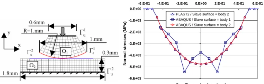
In this numerical test, one considers the contact problem shown in Figure 6. The

1

Ω domain is a part of a disc of 1 mm radius, the Ω1

domain is a rectangle of 1.8 mm x 0.3 mm. On each domain, the behavior law is that of Hooke for the isotropic and homogeneous materials. For k=1,2

, ) u ( 1 E ) u ( ) 1 )( 2 1 ( E ) u ( k k ij k k k k mm ij k k k k k k ij ε ν + + ε δ ν + ν − ν = σ [30]

(13)

-6.E+03 -5.E+03 -4.E+03 -3.E+03 -2.E+03 -1.E+03 0.E+00

-6.E-01 -4.E-01 -2.E-01 0.E+00 2.E-01 4.E-01 6.E-01

Curvilinear abscissa (mm) N o rm a l s tr e s s e s ( M P a )

PLAST2 / Slave surface = body 2 ABAQUS / Slave surface = body 1 ABAQUS / Slave surface = body 2

Figure 6. Finite element model Figure 7. Normal stresses with the local

type approach

The Ω1

domain is embedded in the 2

u

Γ boundary. The displacement imposed on

1 u

Γ is vertical and its value is -0.1581mm. The displacement of 1

u

Γ versus time is a

parabolic trajectory. Its maximum value corresponds to the time where the derivative is zero.

On each solid, one uses rectangular finite elements of the Q1 type (4 node quadrangles) or of the Q2 quadratic type (8 node quadrangles) in plane strains (Ciarlet, 1978). Let us note that the normal and tangential stresses are represented on each figure for a maximum indentation of -0.1581mm.

5.1.1. The local type approach: comparison of PLAST2 and ABAQUS_Standard codes

The aim is to compare PLAST2 and ABAQUS codes on a problem of contact without friction using the classical node-on-segment approach. This allows us firstly to validate the PLAST2 code and to show the limits of the local type approach for dealing with the contact conditions. Let us note that to solve problem [27] using a

dynamic code, one replaces the displacement cycle imposed on 1

u

Γ by a very weak

vertical speed (damping and inertia terms are therefore negligible) subjected to the same surface that puts the two solids under the same deformation cycle. Since the

contact surface deforms during this cycle, it is necessary to update the 1 2,1

G nd a G coupling matrixes at each time step increment.

Figure 7 represents the distribution of the contact normal stresses for a maximum

indentation when 1

c

Γ or 2

c

Γ is the slave surface. One will note the similarities of the

stresses calculated by the two codes and the asymmetrical results obtained when the slave surface is changed. It is clear that on this test the local type approach has shown its limits.

(14)

5.1.2 The global type approach in PLAST2 with Q1 finite elements type

In this paragraph, another technique to approximate contact problems implemented in PLAST2 is presented, called global type approach. One considers first of all the problem of contact without friction. This involves studying the

behavior of the global type approach whether 1

c

Γ or 2

c

Γ is chosen as a slave surface.

By considering the case of piecewise constant multipliers on the contact interface

( 0

h

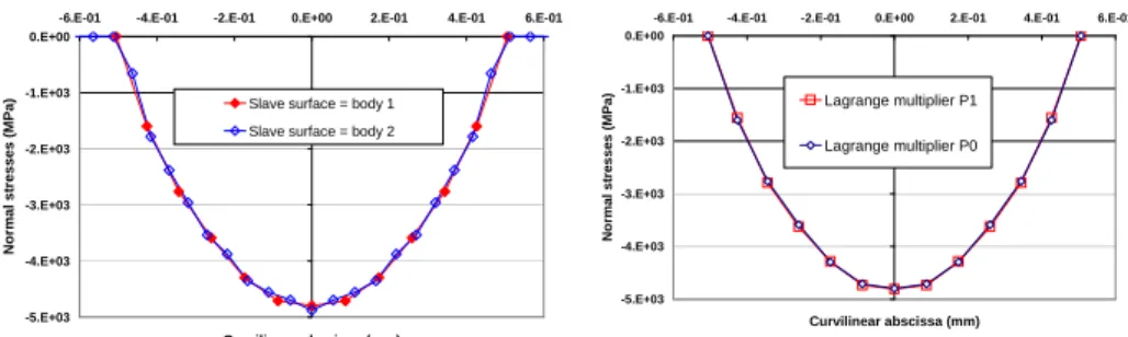
M ), the symmetrical behavior of the global type approach compared to the local one is observed on the distribution of the contact stresses (Figure 8) obtained for the

maximum indentation and for the choice of whatever slave surface ( 1

c Γ or 2 c Γ ). -5.E+03 -4.E+03 -3.E+03 -2.E+03 -1.E+03 0.E+00

-6.E-01 -4.E-01 -2.E-01 0.E+00 2.E-01 4.E-01 6.E-01

Curvilinear abscissa (mm) N o rm a l s tr e s s e s ( M P a

) _{Slave surface = body 1}

Slave surface = body 2

-5.E+03 -4.E+03 -3.E+03 -2.E+03 -1.E+03 0.E+00

-6.E-01 -4.E-01 -2.E-01 0.E+00 2.E-01 4.E-01 6.E-01

Curvilinear abscissa (mm) N o rm a l s tr e s s e s ( M P a ) _{Lagrange multiplier P1} Lagrange multiplier P0

Figure 8. Normal contact stresses

(maximum indentation) when 1 c

Γ or

2 c

Γ is the slave surface with the global type approach

Figure 9. Normal contact stresses

( 0 hn hn M M = or 1 hn hn M M = ) for 1 c Γ slave surface

The comparison of figures 7 and 8 shows that the global type approach makes the management of the contact more symmetrical when slave surfaces are interchanged.

On figure 9, one will note the similarities of the contact normal stresses when

0 hn hn M M = and 1 hn hn M

M = (P0 and P1 multipliers respectively).

Let us now consider the case of a problem of contact with Coulomb’s friction. One has to insure the correct behavior of the global type approach by using the

different convex approximations ( 0

h h M

M = or 1

h h M

M = ) linked to normal and

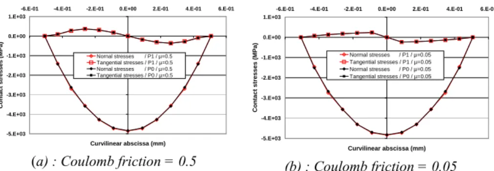
tangential stresses. In this case, the preceding comments apply. In particular, the shape of the normal and tangential stresses is similar (Figure 10) for the two types of

(15)

-5.E+03 -4.E+03 -3.E+03 -2.E+03 -1.E+03 0.E+00 1.E+03

-6.E-01 -4.E-01 -2.E-01 0.E+00 2.E-01 4.E-01 6.E-01

Curvilinear abscissa (mm) C o n ta c t s tr e s s e s ( M P a ) Nornal stresses / P1 / µ=0.5 Tangential stresses / P1 / µ=0.5 Nornal stresses / P0 / µ=0.5 Tangential stresses / P0 / µ=0.5 (a) : Coulomb friction = 0.5 -5.E+03 -4.E+03 -3.E+03 -2.E+03 -1.E+03 0.E+00 1.E+03

-6.E-01 -4.E-01 -2.E-01 0.E+00 2.E-01 4.E-01 6.E-01

Curvilinear abscissa (mm) C o n ta c t s tr e s s e s ( M P a ) Normal stresses / P1 / µ=0.05 Tangential stresses / P1 / µ=0.05 Normal stresses / P0 / µ=0.05 Tangential stresses / P0 / µ=0.05 (b) : Coulomb friction = 0.05

Figure 10. Normal and tangential stresses ( 0

hn hn M M = or 1 hn hn M M = ) for different Coulomb friction

5.1.3. The global type approach in PLAST2 with Q2 finite elements type

The global type approach has been implemented into PLAST2 for quadratic finite elements Q2 to simulate the problem of contact with Coulomb’s friction between two elastic solids (see (Moussaoui, 1992)) for a problem of unilateral contact without friction).

The convexes of Lagrange multipliers are continuous piecewise linear functions

( 1

h

M ) or constant piecewise functions ( 0

h

M ) on Γc . The use of such finite elements

gives hope for a better precision of calculation compared to rectangular or linear elements (Moussaoui, 1992). Figures 11 and 12 validate the correct behavior of the global type approach for problems of contact with or without friction. In the same manner for finite elements of the Q1 type, the results are identical for the Lagrange

multipliers 0 h h M M = or 1 h h M M = . -5.E+03 -4.E+03 -3.E+03 -2.E+03 -1.E+03 0.E+00

-6.E-01 -4.E-01 -2.E-01 0.E+00 2.E-01 4.E-01 6.E-01

Curvilinear abscissa (mm) N n o rm a l s tr e s s e s (M P a ) Q2 elements/ Multipliers P0 Q1 elements/ Multipliers P0 -5.E+03 -4.E+03 -3.E+03 -2.E+03 -1.E+03 0.E+00 1.E+03

-6.E-01 -4.E-01 -2.E-01 0.E+00 2.E-01 4.E-01 6.E-01

Curvilinear abscissa (mm) C o n ta c t s tr e s s e s ( M P a ) Normal stresses / Q2-P0 / µ=0.05 Tangential stresses / Q2-P0 / µ=0.05 Normal stresses / Q2-P1 / µ=0.05 Tangential stresses / Q2-P1 / µ=0.05

Figure 11. Normal stresses

( 0

hn hn M

M = ) for Q1 and Q2 element type without friction

Figure 12. Normal and tangential

stresses ( 0 hn hn M M = or 1 hn hn M M = )

(16)

5.2. Second numerical test

In the case of contact with friction of a deformable body on a rigid surface, one

studies numerically the performance of the methods shown above for 0

h h M M = and 1 h h M

M = . The numerical tests have been carried out on the finite element code

PLAST2. In the numerical tests, the behavior law is that of Hooke for isotropic and homogeneous materials , ) u ( 1 E ) u ( ) 1 )( 2 1 ( E ) u ( ij mm ij ij ε ν + + ε δ ν + ν − ν = σ [31]

with E=7.104 MPa et ν=0.3.

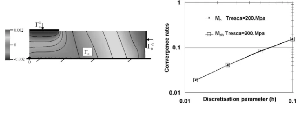
The Ω domain is a rectangle measuring 1.3 mm x 0.3 mm. The discretisation is

carried out with finite rectangular elements of the Q1 type in plane strains. The origin of the curvilinear abscissa is defined from the point O in the trigonometric

direction. A total displacement of 2.10-3mm is imposed on the 1

u

Γ and 2

u

Γ (see

Figure 13). The horizontal displacement is null on 1

u

Γ . The vertical displacement on

2 u

Γ is free which enables a detachment of the deformable body for a curvilinear

abscissa superior to 0.7mm (see Figure 15.a). The Tresca threshold stress is equal to 200MPa.

Figure 13. Vertical displacement on

the reference mesh

Figure 14. Convergence rates of

the two approach 0 h h 0 M M = and 1 h h M M =

(17)

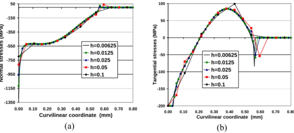
-1350 -1150 -950 -750 -550 -350 -150 50 0.00 0.10 0.20 0.30 0.40 0.50 0.60 0.70 0.80 Curvilinear coordinate (mm) N o rm a l s tr e s s e s ( M P a ) h=0.00625 h=0.0125 h=0.025 h=0.05 h=0.1 (a) -200 -150 -100 -50 0 50 100 0.00 0.10 0.20 0.30 0.40 0.50 0.60 0.70 0.80 Curvilinear coordinate (mm) T a n g e n ti a l s tr e s s e s ( M P a ) h=0.00625 h=0.0125 h=0.025 h=0.05 h=0.1 (b)

Figure 15. a. Normal ; b. tangential stresses for various h and for 0

h h M

M =

Having no analytic solution for the problem treated, the u−uh error in the

energy is numerically estimated by uref −uh . The reference solution is calculated

on a reference mesh containing 9678 elements.

On Figure 14 the convergence order of the different methods for different discretisation parameter h is represented. It can be seen that the convergence is similar for the two approaches. On Figure 15, one can see that the normal stress is not a negative function over all the interface, this is due to the use of slightly negative Lagrange multipliers. However this method enables the singularities of the stresses edges to be attenuated.

5.4. Third numerical test

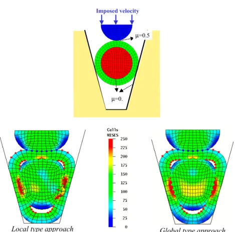
This test enables the global type approach to be validated when compared to the local one, in the case of a simulation of three deformable bodies in contact with one another and with a rigid surface (Figure 16). The bodies have an elasto-plastic

behaviour (

(

2 p

)

0.03

eq =348.210 +ε

σ − _{). Penetrations of the master nodes into the slave}

surface appear in the simulation using the local type approach and they generate a divergence of the calculation whereas the simulation with the global one is carried out without problems.

(18)

Imposed velocity

µ=0.

µ=0.5

Local type approach _{Global type approach}

Figure 16. Comparison between local and global type approach on a forging

simulation of three deformable bodies

6. Conclusion

For the management of a problem of friction contact with the mortar-finite element method and for the construction of a matrix expressing the friction contact of deformable bodies, one can choose form functions (linked to Lagrange multipliers) which are continuous piecewise linear (P1) or constant piecewise (P0). These two approaches have been implemented in PLAST2. Mathematically and numerically on problems of contact with friction, the results of normal and tangential contact stresses are similar when using both approximations (P0 or P1) of Lagrange multipliers.

For a discretisation with quadrilateral elements of the Q1 or Q2 type, it has been established on various numerical tests, that the mortar-finite element method makes

(19)

the management of the contact much more symmetrical when slave surfaces are exchanged, thus closer to physics. Finally, it has been shown that the formulation of this global type approach is also appropriate for Q1 or Q2 finite elements.

7. References

Alart P., Curnier A. “A mixed formulation for frictional contact problems prone to Newton like solution methods”, Comp. Meth. Appl. Mech. Eng., 92, 253-275, 1991.

Baillet L., Sassi T., “Finite element method with Lagrange multipliers for contact problems with friction ”, C.R. Acad. Sci. Paris, Ser. I 334, 917-922, 2002.

Baillet L., Sassi T. “Numerical implementation of differents finite elements methods for contact problems with friction”, C.R. Acad. Sci. Paris, Serie IIB Mechanic, V.331, Issue 11, 2003, pp. 789-796.

Bernardi C., Maday Y. and Patera A.T. “A new nonconforming approach to domain decomposition : the mortar element method”, Collège de France Seminar, Eds H.Brezis, J-L. Lions Pitman, 13-51, 1994.

Bruyère K., Baillet L., Brunet M. “Fiber matrix interface modelling with different contact and friction algorithms”, CIMNE. Edited by : D.R.J.OWEN, E.ONATE and E. HINTON, 1156-1161, 1997.

Chaudhary A., Bathe K.J. “A solution method for static and dynamic analysis of three-dimensional problems with friction”, Computers and Structures, Vol. 37, 319-331, 1986. Ciarlet P.G. The finite element method for elliptic problems. Studies in Mathematics and its

Applications, Vol. 4. North-Holland Publishing Co., Amsterdam-New York-Oxford, 1978.

Coorevits P., Hild P., Lhalouani K., Sassi T. “Mixed finite elements methods for unilateral problems : convergence analysis and numerical studies”, Mathematics of Computation, Vol. 71, No. 237, pp.1-25, 2002.

Duvaut G. et Lions J.-L. Les inéquations en mécanique et en physique, Dunod, Paris, 1972. Haslinger J., Halavàcek I. “Approximation of Signorini problem with friction by a mixed

finite element method”, J. Math. Anal. Appl., 86, 99-122, 1982.

Hild P. Problèmes de contact unilatéral et maillages éléments finis incompatibles, Thèse N° d’ordre : 2903, Doctorat de l’Université Paul Sabatier, 177 pages, 1998.

Hild P. Numerical implementation of two nonconforming finite element methods for unilateral contact, Comp. Meth. Appl. Mech. Eng., 184, pp.99-123, 2000.

Hild P., Laborde P. “Quadratic finite element methods for unilateral contact problems”, Applied Numerical Mathematics, 41, 401-421, 2002.

Klarbring A. “A mathematical programming approach to three dimensional contact problems with friction”, Comp. Meth. Appl. Mech. Eng., Vol. 58, 175-200, 1986.

(20)

Kikuchi N., Oden J.T., Contact problems in elasticity : A study of variational Inequalities and Finite Element Methods. SIAM ; Philadelphia ; 1988.

McDevitt T.W. and Laursen T.A. “A mortar-finite element formulation for frictional contact problem”, Int. J. Numer. Meth. Engng, 48, 1525-1547, 2000.

May H.-O. “The conjugate gardient method for unilateral problems”, Computers and structures, 12 (4), 595-598, 1986.

Moussaoui M., Khodja K. “Régularité des solutions d'un problème Dirichlet-Signorini dans un domaine polygonal plan”, Commun. Part. Diff. Eq., 17, 805-826, 1992.

Raous M., Barbarin S., “Conjugate gradient for frictional contact”, Proceeding of the Contact Mechanics International Symposium, A. Curnier (Ed.), 1992.

Rebel G., Park K. C., Felippa C.A. “A contact formulation based on localized Lagrange multipliers: formulation and application to two-dimensional problems” International Journal for Numerical Methods in Engineering Vol 54, Issue: 2, 2002, Pages: 263-297 Simo J.C., Laursen T.A. “An augmented Lagrangian treatment of contact problem involving

friction”, Computers and Structures, 42, 97-116, 1992.

Wriggers P., “Finite element algorithms for contact problems”, Archives of Computational Methods in Engineering, 1-49, 1995.

Wriggers P., VU Van T., Stein E., “Finite element formulation of large deformation impact-contact problems with friction”, Computers and Structures, Vol. 37, 319-331, 1990. Zhong Z., Mackerle J. “Static problems-a review”, Engineering Computations, 9, 3-37, 1992.