Diffusion-driven flows due to an obstruction layer

Diffusion-Driven Flows Due to an Obstruction Layer

by

Michael R. Allshouse

Submitted to the Department of Mechanical Engineering

in partial fulfillment of the requirements for the degree of

Bachelor of Science in Mechanical Engineering

at the

MASSACHUSETTS INSTITUTE O Y

June 2008

@

Massachusetts Institute of Technology 2008. All rights reserved.

Author ...

/ - .. I .... ... J.. .. . .. . ...

Department of Mechanical Engineering

May 9, 2008

Certified by...

... v .

..

...

. ...

Thomas Peacock

Associate Professor of Mechanical Engineering

Thesis Supervisor

Accepted by ..

John

... H....

Lie nhard V

Professor of Mechanical Engineering

Chairman, Undergarduate Thesis Committee

SSACHLUSETTS INSTITUTE OF TECHNOLOGY

AUG 14

2008

LIBRARIES

Diffusion-Driven Flows Due to an Obstruction Layer

by

Michael R. Allshouse

Submitted to the Department of Mechanical Engineering on May 9, 2008, in partial fulfillment of the

requirements for the degree of

Bachelor of Science in Mechanical Engineering

Abstract

With the confirmation of experiments, two new concepts about diffusion-driven flow are discussed and demonstrated. Although Phillips-Wunsch flow has been shown to exist along sloping boundaries, it is shown here that even an obstruc-tion layer with only vertical walls produces a type of diffusion-driven flow. This is demonstrated through the execution of a dye test. Additionally, the influence that impermeable obstructions have on the density evolution of a stratified fluid is developed theoretically and demonstrated experimentally. With the use of two different types of obstruction layers, the theory is shown to accurately predict the density evolution.

Thesis Supervisor: Thomas Peacock

Acknowledgments

To my friends and family for their support during this process.

Of course, Professor Peacock for all his help and guidence during this work. Generous funding was provided by the Paul Gray fund.

Offering Matlab assistance, Manikandan Mathur provided great insight for the numerics

Design tips and manufaturing help from Pat McAtamney helped make the plates a reality.

Contents

1 Introduction

1.1 Diffusion-Driven Flow Theory ...

2 Stratification Evolution

2.1 Governing Equation ... 2.2 Solution Method ...

2.2.1 Sturm-Liouville Method ... 2.2.2 Direct Numerical Method ...

2.2.3 Comparison of Methods ... 2.3 Design ... 2.3.1 Particle Layer ... 2.3.2 Flat Layer ... 2.3.3 Support Structure ... 2.3.4 Lid ... 2.4 Procedure ...

2.4.1 Assembly of Obstruction Layer and 2.4.2 Adding The Stratified Water ...

2.4.3 Probe Installation and Calibration 2.4.4 Measurement ...

2.5 Results ...

2.5.1 Particle Layer Results ... .

2.5.2 Flat Layer Results ... ..

2.5.3 Density Gradient Evolution ...

7 17 . .. .. .. . .. .. . .. . 17 .. . .. .. . .. .. . .. . 20 .. . .. .. .. . .. . .. . 20 .. . .. .. .. . .. .. .. 22 .. . .. .. . .. .. . .. . 25 .. . .. .. .. . .. .. . . 26 .. . .. .. .. . .. .. . . 26 .. .. . .. .. . .. .. .. 28 .. .. .. . .. .. . .. .. 31 .. . .. .. .. . .. .. .. 32 .. . ... . .. . .. .. .. 32 Installation . ... 32 .. .. .. . .. .. . .. .. 34 . . . 35 .. .. .. . .. .. . .. .. 37 .. .. .. . .. .. . .. .. 38 . .. .. . .. .. .. . ... 38 . . . . . 40

2.6 Conclusion ... ... 3 Flow Visualization 3.1 Theory ... 3.2 Experiment ... 3.2.1 Experimental Components 3.2.2 Experimental Procedure . 3.3 Results ... 3.4 Conclusion ...

A Direct Numerical Simulation Source Code

B Detailed Drawings

C Labview Data Collection

. . . . . . . . . . . . . . . . . . . .°

. . . . . . . . . . . . . . . . . .° . .

. . . . . . . . . . . . . . . . . . . .°

. . . . . . . . . . . . . . . . . . . .°

List of Figures

1-1 Sketch of the development of Phillips-Wunsch flow.[4] ... 15

2-1 Differential slice of fluid system. Sloping walls (bold) induce a diffusion-driven flow up the wall (solid arrow). This flow up the wall requires a return flow (dashed arrow). Looking at a differential slice where the coordinate is taken in the vertical, there are two levels (dashed lines) x and x + dx. ... ... 18

2-2 Trap Inside the Tank ... 27

2-3 Basic Frame ... . 29

2-4 Modified Frame .. .... ... .. 29

2-5 Top view of the particle layer with the top mesh and frame removed. 29 2-6 Side view of the particle layer... 30

2-7 Sketch of the side view of the particle layer. . ... 30

2-8 The liquid fraction for a system containing the particle layer. Height is scaled by the system height... .... 30

2-9 Top view of the flat layer. ... 31

2-10 The liquid fraction for a system containing the flat layer. Height is scaled by the system height... .. 31

2-11 Sponge, Stopper and Straws ... 33

2-12 Two Bucket System ... 34

2-13 Pump used to pump water from the bucket to either the other bucket or the tank ... ... 35

2-15 An example calibration test ... ... 37 2-16 The simulated evolution of a density profile containing the particle

layer over a four day period ... ... 39 2-17 The measured evolution of a density profile containing the particle

layer over a four day period ... 40 2-18 Entire profile comparison between simulated and measured density

profiles containing the particle layer after one day. ... . 41 2-19 Comparison between simulated and measured density profiles

con-taining the particle layer after one day. . ... 41 2-20 Comparison between simulated and measured density profiles

con-taining the particle layer after two days. . ... 42 2-21 Comparison between simulated and measured density profiles

con-taining the particle layer after three day. . ... 42 2-22 The simulated evolution of a density profile containing the flat layer

over a four day period ... 43 2-23 The measured evolution of a density profile containing the flat layer

over a four day period ... 43 2-24 Comparison between simulated and measured density profiles

con-taining the flat layer after one day. . ... . 44 2-25 Comparison between simulated and measured density profiles

con-taining the flat layer after two days. ... ... 44 2-26 Comparison between simulated and measured density profiles

con-taining the flat layer after three day. ... ... 45 2-27 Comparison between simulated and measured density gradients for

a system containing the flat layer ... .. 46 2-28 Comparison between simulations of a systems with and without an

obstruction layer ... . .. ... .. 46 10

3-1 A sketch of the isopycnals for a stratification in the presence of an obstruction with a vertical hole in it. The obstruction is in the thick black strip. The isopycnals are the lines. ...

3-2 A top view of the obstruction layer used for the dye experiment, the hole layer . ...

3-3 The device used to pump the dye into the trough. This contains a syringe filled with dye that is compressed by a rotating threaded rod. 3-4 Side view of the rod and tube during the injection process

3-5 The initial image of the dye position . . . . 3-6 Dye location after 4 hours of exposure ... . .

3-7 Dye location after 8 hours of exposure ... . .

3-8 Dye location after 12 hours of exposure . . . . B-1 Engineering drawing for original frame ...

B-2 Engineering drawing for modified frame . . . . B-3 Engineering drawing for flat obstruction layer ... B-4 Engineering drawing for hole obstruction layer ...

C-1 Labview interface for data collection ...

C-2 Labview circuit used to take data...

. . . . . . 52 . . . . . 56 . . . . . 56 . . . . . 57 . . . . . 57 . . . . . 64 . . . . . 65 . . . . . 66 . . . . . 67

Chapter 1

Introduction

A remarkable phenomenon arises along impermeable structures within a

strat-ified fluid. Phillips [5] and Wunsch [7] independently found that along a sloping impermeable boundary a flow develops if there is a density stratification within the fluid. This flow is due to the conflict between the no-flux boundary condi-tion and the influence of gravity. This inequillibrium induces flow along the wall called Phillips-Wunsch flow which falls into the general category of diffusion-driven flows.

This phenomenon has been studied by a number of researchers and it is also possible that it may be influential in a couple environmental settings. Peacock, Stocker, and Aristoff studied the influence that the angle of the wall had on the flow velocity [4]. They were able to show a close correlation between the theoretical and experimental measurements for angles larger than five degrees. They also showed that the velocity tends to zero as the angle goes to zero. Peacock has also shown the power of diffusion flows in his studies of the "diffusion fish" [3]. This research has shown that the diffusion flows over a sloping surface are so great that it can actually propel an object forward. Baidulov et. al. have done significant study on the diffusion-driven flow over a sphere [1]. They were able to identify the flow structures around a sphere isolated in a stratified fluid. It is believed that in addition to these studies that diffusion-driven flow may play a role in the studies of diffusion through porous media as well as the possible development of layering

within bodies of water.

While much of the work done on diffusion-driven flows has looked at systems where entire walls are sloped, this work tries to isolate the influences that an ob-struction layer has on a stratified fluid. This obob-struction layer in nature is made up of impermeable particles. It is believed that the introduction of non-vertical obstructions will induce diffusion-driven flows within the fluid. Meaning the in-troduction of these obstruction layers could substantially influence the way the diffusion through the system occurs. While it is expected that sloped walls of par-ticles will cause diffusion-driven flow, the study of obstruction layers with only vertical walls provides insight as well.

The objective of this thesis is to develop the two new findings made in research-ing these obstruction layers. The first is the development of a mathematical model which accurately predicts the density evolution within the system taking into ac-count an obstruction layer. This model is then simulated and tested against exper-imental results. The other new idea is the isolation of diffusion-driven flow within systems containing no sloped walls. This concept is developed theoretically, and then it is shown through experimental results.

1.1 Diffusion-Driven Flow Theory

As mentioned there are two conflicting physical influences: gravitational direc-tion and no-flux condidirec-tion. For hydrostatic equilibrium, the density of the fluid normal to the direction of gravity must be uniform. This means that if a horizontal cross sectional slice is taken from the fluid, the density along the entire plane must be uniform for there to be hydrostatic equilibrium. The no-flux condition requires that the lines of constant density, isopycnals, are normal to any impermeable wall. The reason for this is that diffusion goes down the density gradient. Since there is no diffusion through and impermeable wall, there can be no density gradient nor-mal to that wall. The problem arises when these walls are not vertical. In the case of sloped walls this hydrostatic equilibrium is broken because the density lines

TI

Figure 1-1: Sketch of the development of Phillips-Wunsch flow.[4] bend from horizontal to be normal to the walls.

Peacock et. al. do an excellent job sketching what is happening physically. Their figure is shown here as Figure 1-1. At the bottom left of the figure it shows the lines of constant density, p, bending to meet the slanted wall. With a stratifi-cation in place each of these lines represents a different density. This means that taking a horizontal cross section will not contain a constant density due to the bent isopycnals. This leads to the development of the flow with velocity profile u(rl) shown at the top right of the figure. This velocity profile is based on arguments made by both Phillips [5] and Wunsch [7].

Chapter 2

Stratification Evolution

Within bodies of water there is often a stratification, a variation in the density of the fluid as a function of height. While this density variation can be due to variations in temperature, the focus of this work will be on density variations due to changes in salinity. This stratification will change over time due to diffusion as well as other factors.

With the understanding of how diffusion-driven flow arises, the development of its influence on the stratification evolution is looked at. In his study on boundary-driven mixing, Woods looks at the influence that diffusion-boundary-driven flow has on the density evolution of the system [6]. He develops a governing equation for the density evolution accounting for the presence of diffusion-driven flow occurring throughout the system, and he briefly comments on the possibility that imper-meable particles may have an effect on the density evolution of the system. This chapter goes through the development of a governing equation for the stratifica-tion evolustratifica-tion taking into account an obstrucstratifica-tion layer. It goes on to describe an experiment to test this theoretical result.

2.1

Governing Equation

The governing equation is based on an approach developed by Woods [6], and will also use some of the assumptions that he made in his derivation. In his paper

- x+ dx

Figure 2-1: Differential slice of fluid system. Sloping walls (bold) induce a diffusion-driven flow up the wall (solid arrow). This flow up the wall requires a return flow (dashed arrow). Looking at a differential slice where the coordinate is taken in the vertical, there are two levels (dashed lines) x and x + dx.

he states that the two assumptions he makes in his model are that the particle spacing is much greater than the boundary layer of the diffusion-driven flow and that the density is only a function of z. Given that the boundary layer that develops for these flows is on the order of a fraction of a millimeter, this assumption appears to hold. Given the filling method, described later, the density function varies only with z far away from the wall which is what the assumption requires.

To develop the governing equation a differential slice, shown in Figure 2 - 1,

from a general system is analyzed. The two walls on the outside define the range of the whole system and has a total cross section defined as, A(z). The differential slice shows the diffusion-driven flows and the return flow that develops.

Since this study takes into account the possibility that there are obstructions, a function is created to include this factor. The fraction of the cross section that is water is the only portion through which diffusion can take place. This leads to the creation of the function O(z) termed the liquid fraction function.

In order to develop the governing equation, the basic physical concepts of vol-ume and mass conservation must be analyzed. For the volvol-ume conservation, it is know that the Phillips-Wunsch flow will be taking place along all non-vertical walls of the system. The overall volume flux of the Phillips-Wunsch flow with the function Q(z). From the shape of the system all the Phillips-Wunsch flow will be going from bottom to top. This leads to a volume reduction at the bottom of the

I

I

I I

system. Since a vacuum is not created in the system, there has to be a method of restoring the volume at the bottom of the tank. A result of the Phillips-Wunsch flow is a return flow through the center of the system. The average velocity of this return flow is defined to be W(z). This average is taken over a range of all the liquid cross section outside of the Phillips-Wunsch boundary layer. Since this boundary layer is so small it can be assumed that the return flow essentially goes through the entire fluid area, A(z)4(z). These two flows are the only contributors to the change in volume, so to satisfy the volume conservation the volume flux of the two are equal to each other

Q(z) = W(z)A(z)¢(z). (2.1)

To satisfy mass conservation, all the contributions to the change in mass of a differential slice must be accounted for. There are a number of mass flows occur-ring in this system. Looking at just the top of the system, there is mass flowing out of the system due to the Phillips-Wunsch flow, mass entering the system due to the return flow, and mass leaving due to the diffusion down the density gra-dient. At the bottom of the Phillips-Wunsch flow bring mass into the system, the return flow removes mass, and mass enters due to the diffusion down the density gradient. Overall the mass rate of change for the differential slice is

(pA) _ Ap1 O(pQ) _{+(pWA) (2.2)}

=

&t

8z I 8z

8z

az

Using Equation 2.1, this simplifies to

&- - A 9z A . (2.3)

In addition to the governing equation the boundary conditions and the initial value has to be taken into consideration. The two boundary conditions that are accounted for are both no-flux conditions. At the top of the system, there is no diffusion through the free water surface, meaning the density gradient must be

zero here. The same is true for the bottom of the system. The initial value used to develop the evolutions is the initial density profile.

2.2 Solution Method

There are two different methods to determining the solution to the governing equation. Both methods require the use of numerical methods in order to be ap-plicable to general liquid fraction functions. The first method described breaks the partial differential equation into two ODE's by means of a separation of variables. One ODE has the property of being a Sturm-Liouville problem. This allows for the development of modal shapes and solutions that apply to any initial profile. These mode shapes and numbers are then used to create a density profile evolution. The other method is a direct numerical interpretation of the problem. In this case the partial differential equation is solved directly through the use of a finite difference method. Both methods offer unique benefits and will be compared.

2.2.1

Sturm-Liouville Method

For the system being considered there is a constant overall cross section mean-ing that the function A(z) can be eliminated from Equation 2.3. The governmean-ing equation is now broken down by a method of separation of variables. With the assumption that the density function can be defined as

p(z, t) = g(t)h(z), (2.4)

the governing equation can be manipulated to be

dg A

+ -g = 0,

(2.5)

20

where A is the eigenvalue or mode number. The two different differential equa-tions can be defined as the temporal and spatial differential equaequa-tions respectively. The solutions to the spatial differential equation are called the mode shapes. Each mode shape corresponds to a distinct mode number, but all the mode shapes must satisfy the boundary conditions.

=L 0 (2.7)

aZ z=0,L

The solution to Equation 2.6 is trivial but there is a different solution for each mode number. The temporal and spatial solutions are paired up based on mode number. Since the system is linear these solutions can be superimposed on each

other. After combination and superposition, the solution becomes 00

p(z, t) = cj hj(z) exp -( t (2.8)

j=1

where hj(z) is the function of the jth mode shape, A3 is the jth mode number,

and cj is the coefficient which causes the equation to satisfy its initial condition, the initial stratification. At this point there are an infinite number of coefficients yet to be determined, and the initial condition has yet to be taken into account. One property of the solutions to the Sturm Liouville problem is that all the mode shapes are orthogonal to each other if the liquid fraction function is continuous and everywhere differentiable. Using this property the coefficients to the solution are defined as

ci = L h(z)p(z, 0)(z)dz

(2.9)

To simulate the system using this method a program that solves for the modes used in Equation 2.8, and project these mode shapes onto the initial condition had to be developed. The program uses the Matlab code bvp4c and the boundary con-ditions to find the mode shapes and mode numbers of the solution. The mode shapes are then scaled so their summation will reproduce the initial value distri-bution. Finally the program combines the mode shapes with the corresponding

temporal solution and displays the linear combination of a set number of modes.

2.2.2 Direct Numerical Method

To solve directly from the partial differential equation, the system will have to be discretized both space and time. The definition of the derivative will also have to be assumed. With a discrete system it is not possible to infinitesimally approach a point from both sides, thus the derivative has to be redefined. Although these two things bring in inherent errors, the code is able to compensate if it can insure that the numerical method is stable. Given the system in Equation 2.3, a new func-tion is created for simplicity

G(z) = O(z)P (2.10)

Using this substitution Equation 2.3 is changed into

Op

n OG(z)

-• = -

dt

az

Temporal Approximation

Since the spatial terms leave first order error it is easiest to use the temporal approximation

p) _(2.12)

at At

There are now two indicators for p. The superscript term represents the time step, and the subscript term represents the spatial location.

Spatial Component

The spatial element is broken into N equally spaced points spanning the system at a distance Az apart. Using this discretization the derivative is redefined as

OG(zi) _ G(zi+l) - G(zi-₁₎

Sz(2.13)

where

Gp(zi+i) = 3p(z+,₁) - 4p(z2) + p(zi-,) (2.14)

G(zi 1) = (zxi+i) = -(zj+ ₁) (2.14)

8z 2Az

similarly

G(zi-1) = () Zp(zi-1) -p(zi+) + 4p(zi) - 3p(zi_.) (2.15)

az 2Az

Using a modified notation, for example

q(Zi-1) = Oi-1 (2.16)

Equations 2.14 and 2.15 can be substituted back into Equation 2.13 and get the result

~i [0 ¢i 4 Az2 _{i [(3i+1 + i-1)pji+l - 4(Ok+1 +}

•i-1)pi + (0i+1 + 304_1)p-_1]

(2.17) This equation can be used to represent all the interior points of the system (i.e. for

z2 to ZN-1), but a different equation has to be used to account for the boundary

conditions at the end points of the system.

Boundary Condition

At the most extreme points the fact that the density must be constant will be taken advantage of and the standard differential becomes

dp(Zl) -- p(z3) + 4p(z2) - 3p(z) (2.18) = 2(2.18) 8z 2Az and Op(zN) -- P(ZN-2) - 4p(ZN_1) + 3p(zN) Z = 2Az (2.19)

Given a no-flux boundary condition at both the free surface and the bottom, the derivatives can be set to zero. This creates the final two equations that will be used

to solve for a density vector.

-P(z3)

-

P(2) + P(Z1)

= 0

3

3

1)

+ P(ZN)

=

0

Implementation of the Approximations

There are a number of ways to combine the above approximations to simu-late the evolution of the system, but taking into account speed and accuracy the implicit method seems to be the first choice. This method combines the approxi-mations to be

1+1 1

P _{P 4z} 2

i

[(30+1 + i-1

Using the substitution

)pi+

-

4(q5+1

+

+

(0ij1 +

30i-1)P_1+11

(2.22) KAt

A

S1+1

Making the substitutions lead to

Li - -A 30- 1 + _j_

Oi

i

Oi

_O

_I

This allows for the creation of the matrix 1 -4/3 1/3 0 0 L2 C2 R2 0 0 0 L3 C3 R3 0 0 0 LN-1 CN-1 RN-1

0 0

1/3 -4/3

1

Using the notation

[A]b = C (2.29)

the matrix of multiplying factors will be named [A], the vector b is the new density vector, and the vector ' is the modified old density vector. The vector C' takes the old density vector and replaces the first and last entries with zeros to account for the boundary conditions. The full code used for the simulation of the density over time is included in Appendix A.

2.2.3 Comparison of Methods

Both methods are capable of developing solutions, but there are strengths to both. The Sturm-Liouville method has the ability to develop evolutions rapidly if the liquid fraction function remains the same. The mode shapes and numbers are developed based only on the equation itself which dominates the run time and not on the initial profile. The modes are then projected onto any type of initial profile giving it the ability to simulate profile evolutions for multiple initial profiles without having to develop more mode shapes and numbers. The direct numerical method does not go through the process of developing modes so it reruns the entire code for systems that have the same liquid fraction function. However, it has the ability to simulate solutions for liquid fraction functions that are discontinuous or not everywhere differentiable. Discontinuous liquid fraction functions are not capable of being decomposed into modes since it breaks one of the requirements

for the Sturm-Liouville problem. Both methods were executed on a system with no obstruction layer and were capable of developing accurate simulations compared to the analytic solution. Since the direct method is more flexible, it will be used to simulate profile evolutions.

2.3 Design

In order to test the theory, it was necessary to be able to suspend obstructions in a stratified fluid. There had already been a method developed for the creation of a linear stratification, so the majority of the design necessary to run the experi-ment was focused on adding a fixed obstruction layer. The objective was to have a modular system so that multiple obstruction layers could be placed with the same apparatus.

2.3.1

Particle Layer

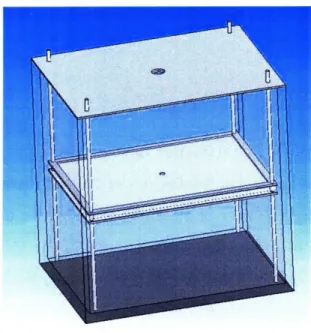
The first type of obstruction layer was a layer of acrylic particles. There had been attempts in the past to simply place the particles at the bottom of the tank and allow them to find their neutrally buoyant height. Assuming all the particles have the same density, they should theoretically end up at the same height. A problem with this is that there was a slight variation in the height of the particles due to variations in density, and if an air bubble developed in the water and attached to a particle it would cause the particle to move. The objective was to design an apparatus that had the capability of fixing the particles in place at a desired height. A general concept had already been thought up and needed further develop-ment and fabrication. The idea was to contain the particles in a mesh trap that would be supported by a rod system. After some modification, a final design was agreed upon and a solid model is featured in Figure 2-2. The design includes a frame, a mesh support, and four rod supporting the system at the comers. The particles would be attached to the mesh making them fixed in all directions.

Figure 2-2: Trap Inside the Tank

The purpose of the trap was to contain an obstruction layer of impermeable particles. The acrylic particles would be glued to a plastic mesh that would fix their position. To support this mesh, a frame had to be designed that would provide support and offer a way for the mesh to be located vertically.

The frame would be two thin pieces of acrylic that would be on top and below the obstruction and mesh layer. There were two concepts of the frame. The first was to have a rectangle with the center removed as shown in Figure 2-3. This frame offered support to the mesh only on the outside and had the ability to be mounted by a rod system. It was found that the weight of the particles in the water caused significant sagging of the mesh. This led to the second version of the frame shown in Figure 2-4. This frame, although it may obstruct the fluid slightly, offered a significant decrease in the amount of sag. The frames were then made of 1/8" thick acrylic and were machined on the water jet. Detailed drawings of the frames are provided in Appendix B.

The final product included the two acrylic frames, two layers of mesh and 480 quarter inch acrylic spheres. A top view of the layout is shown in Figure 2-5, and a side view is shown in Figure 2-6. This particle layer provided the ability

to introduce an obstruction layer that would change the liquid fraction drastically only in a small region.

Particle Layer Liquid Fraction Function

The calculation of the liquid fraction function is straight forward. It is assumed that the layer is level and that the bottom of the obstruction layer is at a height

z = h. Assuming the influence of the frame is negligible, the change in the liquid

fraction is a function of the cross sectional area of the sphere at a given height. Figure 2-7 shows a sketch of one particle. This sketch leads to the cross sectional area of a single sphere to be defined as

AC = r [R2 _{_(R- z + h)}2_{]. (2.30)}

Given that the tank has a constant cross section of At, the liquid fraction function can be defined as

1 z<h

OZ = At-NTr[R2 -(R-zh)2] h < z < h + 2R (2.31)

1 z > h + 2R

where N is the number of particles in the obstruction layer. This profile is shown in Figure 2-8.

2.3.2 Flat Layer

In order to justify the theory experimentally a second obstruction layer was developed. This layer would contain only vertical and horizontal walls to give insight to what occurs in the absence of Phillips-Wunsch flow. To make this layer a 1/2" piece of acrylic would be machined to contain a number of holes. The holes for the rod would be included in this layer so it would be self sufficient. The final layer is featured in Figure 2-9. This flat layer provided a second obstruction layer which modified the liquid fraction profile. An example of a the liquid fraction

Figure 2-3: Basic Frame

Figure 2-4: Modified Frame

Figure 2-6: Side view of the particle layer.

R

r

z = h +2R

z=h

Figure 2-7: Sketch of the side view of the particle layer.

0 0.2 0.4 0.6 0.8 1

z/H

Figure 2-8: The liquid fraction for a system containing the particle layer. Height is scaled by the system height.

Figure 2-9: Top view of the flat layer.

[

I

0 0.2 0.4 0.6

z/H

0.8 1

Figure 2-10: The liquid fraction for

scaled by the system height. a system containing the flat layer. Height is profile with the flat layer is shown in Figure 2-10. A detailed drawing of this is also included in Appendix B.

2.3.3 Support Structure

To support the two obstruction layers the use of simple rod system was devel-oped. At each of the comers of the frame are holes where the rods are placed. The obstruction layers will be constrained from the bottom and top by a corrosion re-sistant shaft collar at all four comers. These collars are tight enough around the rod to prevent any sort of slipping of the layer. This fixes the layer in place which is necessary to accurately simulate the stratification evolution. The tank that was

used had a raised surface at one of the corners so this had to be accounted for in the determination of the rod heights.

2.3.4 Lid

The final piece to the design was to add a lid to the tank. It was found that there is a nontrivial amount of evaporation and surface flow development if the system is left open. Although a complete covering of the tank may be optimal, the lid must have holes in it for the support rods to come through and for a measuring probe to enter the fluid. The lid must sit snuggly inside the tank so that little motion of the trap is possible. The lid was designed to be two 1/8" layers. The lower layer would be cut to fit just inside the tank. The top layer would be cut so that it reaches the outermost edges of the tank. This two layer system provides the ability to simply drop the lid on and have it slide into place.

2.4 Procedure

To set up the experiment there are a number of basic steps. The first is to set up the obstruction layer and place it in the tank. Next is to add the water so the fluid in the tank starts with a linear stratification. In order to measure the density for different depths, a probe is calibrated, placed on a traverse, and lowered into the water to take the measurements. Within each of these categories there are a number of sub-steps. What follows is a detailed outline of the procedure required to set up and carry out the experiment.

2.4.1 Assembly of Obstruction Layer and Installation

The trap itself was designed to be modular. After selecting the test height, one of the shaft collars was placed on each of the four rods taking into account the fact that one rod is on a platform that is about 3 cm high. Next the rods were inserted into the comers of the obstruction. Finally the top collar is placed on the rod so

Figure 2-11: Sponge, Stopper and Straws

that the obstruction layer is secured from the top and bottom. In both cases it is important to get the obstruction layer as level as possible. Even if there is a slight angle to the surface, there is a modification in the liquid fraction function. Being level is especially important for the flat layer case. Since the goal is to attain results for a system where Phillips-Wunsch flow is not expected, the layer has to be level to within a fraction of a degree. Peacock et. al. showed that the Phillis-Wunsch flow velocity tends to zero as the angle decreases below five degrees [4]. There were two methods of achieving this degree of level. The first was to use a fluid level and make sure it was accurate in multiple orientations. The other method included taking pictures and finding the degree of incline using Photo Shop.

Before the obstruction layer can go in a sponge must be placed at the water entry. This sponge acts to spread the injection of water to a larger area and reduce the velocity with which it enters the tank. This allows for a cleaner stratification. The sponge is held in place using a set up shown in Figure 2-11.

At this point it is important to make sure the path the probe will be traveling is clear. A section in the obstruction must be left open so that the the probe can reach the bottom of the tank. With the lid put on the tank, the opening in the obstruction layer needs to be aligned with the hole in the lid. Once alignment is achieved the system is ready for the stratification.

Figure 2-12: Two Bucket System

2.4.2 Adding The Stratified Water

There are a number of steps that need to be taken to add the water. The water is added to the tank through the use of a pumping mechanism that adds water with increasing salinity. This double bucket system was developed by Oster [2] This is how the linear stratification is developed. The water is removed from a two bucket system, Figure 2-12. One of the two buckets, Bucket 1, is filled with 20 liters of fresh water, p = 1000 --, and the other, Bucket 2, is filled with 40 liters of fully saturated water, p - 1200 k.

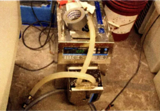
The pumps, Figure 2-13, use a rotary mechanism to move water from Bucket 2 to Bucket 1 and from Bucket 1 to the tank. Before the tank is filled it is important to calibrate the pumps to confirm that they are pumping at the correct rate. If the rate of volume flux is not correct the stratification may not be linear.

The first pump ran the saturated water from Bucket 2 to Bucket 1 at 0.25L/min. Once the saturated water entered Bucket 1, it mixes to create salt water that is pumped to the tank by the second pump at 0.5L/min. As time passes the water in Bucket 1 becomes more and more salty. This corresponds to water pumped in later which will be at the bottom of the tank to be more salty than the top. It takes about 40 minutes to fill the tank up to the required 21 cm height.

Figure 2-13: Pump used to pump water from the bucket to either the other bucket or the tank.

2.4.3 Probe Installation and Calibration

With the tank and stratified water system established, the final step is to take the measurements. The goal of the experiment is measure the density profile over time so a probe that measures density is used each day for four days. The probe used for this experiment was an 80 cm CT probe. The height of the probe at each reading is also measured.

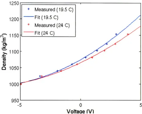
The calibration of the probe is based on the measurements recorded for samples of known density. For reliable calibration of the probe there need to be at least four different water samples of unique densities at two different temperatures. Using the saltwater remaining in Bucket 2, sample jars are filled with salt water of varying densities. Ideally the full range of densities in the tank should be covered by these samples. In order to test at two temperatures, a second set of identical densities must be made. In the experiments run, the average range of densities was from 1000kg/m3 to 1100kg/m3_{. Seven samples were made with densities ranging from}

1000kg/m3 to 1120kg/m 3 with a 20kg/m3 _{interval between samples.}

After all the samples were made each set is placed within its own thermal-bath. One set is taken to a temperature above the tank temperature, while the other bath cools the samples to a temperature lower than the tank's. The thermal-baths work to bring the samples to the desired temperature and keep them there for a desired length of time.

I COU 1200 c 1150 E

,1100

Figure 2-14: An example calibration measurement

After the samples have reached their target temperatures, the CT probe was used to measure both density and temperature. Temperature measurements were also taken with a thermometer, and density measurements were also taken by a densitometer. With the known values of the temperature and density the voltage readings from the CT probe were fit to a curve that would convert a voltage to the appropriate density. An example of one of these calibrations is shown in Figure

2-14.

Once the calibration is complete, the probe was placed on the traverse located over the tank. The traverse is controlled by the computer and can move to a desired location with great accuracy and at a controlled speed. The probe descends into the water and takes the measurement.

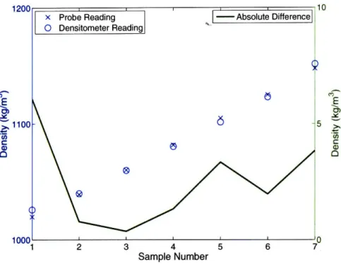
To analyze the reliability of the calibration a test was developed. In order to test the density measurements that are measured by the probe, the reading is com-pared to a reading from the densitometer on the same sample. To make the test as pertinent as possible, the sample jars are set at a temperature approximately equal

CO E 0) C (D 0_t-, o CO_E r• a) 0 1 2 3 4 5 6 7 Sample Number

Figure 2-15: An example calibration test

to that in the tank. Probe readings of the temperature and density of all the samples are taken as well as densitometer readings. This allows for the direct comparison needed. As example test is shown in Figure 2-15. From this test it is shown that the difference between the densitometer reading and the probe reading has a variation of at most 6kg/m3. While this correlates to about a .5 percent difference it is not

ideal. While a better method could be developed, it was felt that even though the variation of the probe may influence the exact numbers it would not significantly influence the shape of the profile.

2.4.4 Measurement

By the time the calibration is completed and the probe has been mounted, any transient motions in the water due to the filling have died out. After all the set up has been complete it was important to take a measurement as soon as possible in order to get the initial density profile. Even though diffusion takes time for noticeable changes in the profile to occur, it is good to have an accurate initial

condition.

After the probe has been lowered to the desired starting position, a VI in Lab-View was run which collected all the data. The interface for the LabLab-View is pre-sented in the Appendix. The way the VI operates was that a program controls both the stepper motor that determines the height and the sensor on the probe. The particular VI that was used in this experiment moved the probe down a frac-tion of a millimeter, paused for five seconds while transients died out, and then took a number of density readings.

The probe-reading the density at a given height produced a non-trivial amount of noise. In order to get a more accurate representation of the profile, a large num-ber of readings were taken at every point. During a typical run, the VI would have the probe take one hundred measurements at a given height in a period of about two seconds. After the measurement was completed, the VI then moved the probe down to its next location, the probe collected more data, and continued down to a desired depth.

The parameters that control this process were the desired depth, the number of depths to analyze, and the number of measurements to take at each depth. The average reading reduced some noise that came up in the reading. After the VI completed the cycle, the probe was returned to its starting position, and would wait until the next run. Based on the simulations it was felt that it was adequate to take measurements once every twenty four hours for four days. This would allow for the capturing of enough readings to confirm the theory.

2.5 Results

2.5.1 Particle Layer Results

The particle layer experiment was the first one run. This experiment was re-peated multiple time while the procedure was perfected. With the continued im-provement of the procedure the results got better. The results discussed here will

E

r•

-0.14 -0.13 -0.12 -0.11 -0.1 -0.09 -0.08

Depth (m)

Figure 2-16: The simulated evolution of a density profile containing the particle layer over a four day period.

be based on one of the most recent trials.

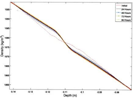
The experimental results proved some of the characteristics discovered while running simulations of the governing equation. The crucial observation is that the density profile deviates from a straight line at the obstruction height. This is different because the way the diffusion equation works is to smooth out all the disturbances. Instead of smoothing out the disturbance it actually amplifies it at the obstruction layer. This was developed in simulation as shown in Figure 2-16 and was shown experimentally as shown in Figure 2-17. Although the exact way the measured results change from day to day may not be exactly the same it is clear that the expected disturbance arises.

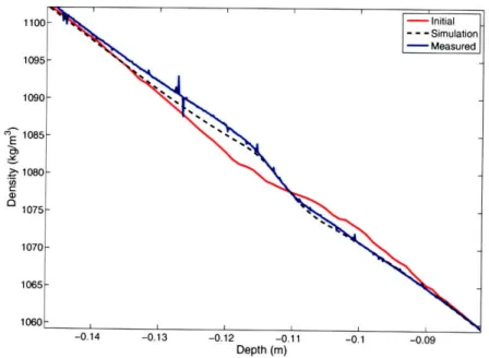
While being able to predict a characteristic difference is important the goal is to find out if the numerical simulation is able to accurately predict the density profile. When looking at the entire profile, Figure 2-18, it is obvious that there is a substantial difference between the theory and the measured results. At the two ends of the profile there are disturbances and thermal flows that develop that cause the density to change at a different rate. This is not taken into account, so it

-0.13 -0.12 -0.11 -0.1 -0.09 -0.08

Depth (m)

Figure 2-17: The measured evolution of a density profile containing the particle layer over a four day period.

is expected that these values will be off. The important part of this experiment is to look at the profile around the obstruction height. Figures 2-19 to 2-21 illustrate the comparison between the measured results and the simulation. Although the exact values are not matched they are accurate to within 5kg/.m3

2.5.2 Flat Layer Results

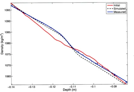
The flat obstruction layer was used in the second round of experiments. By this time the procedure had been perfected and this shows up in the results. The ex-pected result this time was that there would be a sharp change in the stratification at the obstruction height. This shows up both in the simulated results, Figure 2-22, and in the experimental results, Figure 2-23. Again there are disturbances at the two extremes which leads to the concentration on the comparison between the simulated and measured results at the obstruction layer. Figures 2-24 to 2-26 show the evolution and comparison between the two over days one through three. In this case the difference between the two is within 1kg/m3.

E

Depth (m)

Figure 2-18: Entire profile comparison between simulated and measured density profiles containing the particle layer after one day.

Depth (m)

Figure 2-19: Comparison between simulated and measured density profiles con-taining the particle layer after one day.

C

0) E

a2

Depth (m)

Figure 2-20: Comparison between simulated and measured density profiles con-taining the particle layer after two days.

CýE U)

0,

Depth (m)

Figure 2-21: Comparison between simulated and measured density profiles con-taining the particle layer after three day.

Figure 2-22: The simulated evolution of a density profile containing the flat layer over a four day period.

Depth (m)

Figure 2-23: The measured evolution of a density profile containing the flat layer over a four day period.

co)_CO

E

U)

0

Depth (m)

Figure 2-24: Comparison between simulated and measured density profiles con-taining the flat layer after one day.

COE

CO

(U)

-Depth (m)

Figure 2-25: Comparison between simulated and measured density profiles con-taining the flat layer after two days.

C., (I, C 0) 0 -0.13 -0.12 -0.11 -0.1 -0.09 -0.08 -0.07 -0.06 Depth (m)

Figure 2-26: Comparison between simulated and measured density profiles con-taining the flat layer after three day.

2.5.3 Density Gradient Evolution

The predominant feature of the density evolution is the creation of the higher density gradient at the obstruction layer. Since the flat layer shows a higher level of agreement with the model this scenario will be analyzed. The evolution of the den-sity gradient for this particular initial stratification is shown in Figure 2-27. From the figure there is again close agreement between the simulation and the points actually measured. This indicates that the simulation would be a good basis to make predictions. Perhaps one of the more telling plots is a comparison between the density gradient evolution for a system containing the flat layer and one con-taining no obstruction layer. Based on the way diffusion in a system without an obstruction layer acts, the initial density gradient at the center of the system will always be decreasing. Figure 2-28 demonstrates the evolution for two identical systems except for the presence of the flat layer. As predicted the system without the density layer decreases the magnitude of the gradient over time, while the sys-tem with the obstruction layer has an initial increase in gradient that remains for a significant amount of time.

E

CO

Figure 2-27: Comparison between simulated and measured density gradients for a system containing the flat layer

Figure 2-28: Comparison between simulations of a systems with and without an obstruction layer

2.6 Conclusion

The results indicate that the theory seems to match what is actually happening. In the region where only the diffusion-driven flows are expected to be occuring the measured and theoretical data matches very well. While the particle layer does not share the same degree of high accuracy as the flat layer, if experimental results were as refined similar results maybe possible. Almost as important as the actual prediction of densities is the disturbance created at the obstruction layer. Even though the actual numbers were not accurately matched the general shape of the disturbance was. This leads to the belief that at least to a first order the theory is accurate.

While the experiments offered many good results there are areas where there could be marked improvement. For the particle layer, even with the modified layer there is still a slight sag to the obstruction layer. This leads to a slight variation in the liquid fraction function. If stronger supports were added that did not reduce the liquid fraction greatly were added, it is possible the results may be cleaner. The calibration method could also use some improvement. While the calibration generally offers accuracy to within a couple kg/m 3, some of the calibrations have

shown variation from actual to measured of upwards of 6kg/m3.

An interesting conclusion from this result is that the flat layer shows significant change in from a system that has no obstruction layer. This indicates that there is likely a flow of some sorts going on. This belief will lead to the attempt to visualize a possible flow which is done in Chapter 3.

Chapter 3

Flow Visualization

The second concept that was looked into was the flow visualization of flows that develop in the presence of an obstruction layer having only vertical walls. The Phillips-Wunsch flow was known to develop flows along walls that were non-vertical, so it may seem surprising to find that flows also develop in the case where an obstruction layer contains only vertical walls. Through the development of a general theory and the confirmation through experimental results, it was found that a flow directed radially outwards occurs along the top surface of an imperme-able obstruction layer containing a hole in the center.

3.1 Theory

The theoretical development of this study shares many of the same ideas with the development of the Phillips-Wunsch flow. Again the two conflicting condi-tions are the no-flux boundary condition and the direction of gravity. In this case Figure 3-1 illustrates the expected isopycnals. The isopycnals over the center of the hole are horizontal but above the plate they must bend to be vertical to satisfy the no-flux condition. This causes the hydrostatic equilibrium along a plane parallel to the top of the surface. For the top surface, the further from the center of the plate the less dense the water becomes. This leads to the belief that the flow will be radially outwards.

[

Figure 3-1: A sketch of the isopycnals for a stratification in the presence of an obstruction with a vertical hole in it. The obstruction is in the thick black strip. The isopycnals are the lines.

Figure 3-2: A top view of the obstruction layer used for the dye experiment, the hole layer

3.2 Experiment

To capture this phenomenon an experiment is set up so that the flow drags a blue dye along the surface of the plate. This dye is a mixture of water, salt, and dextran dye. The water and salt mixture are made so that the dye is approximately the same density as the water at the obstruction height. The dextran dye adds the blue color to the dye and has the unique property that the coefficient of diffusivity is considerably lower than that of salt in water. This means that any movement of the dye is due to currents within the system.

Figure 3-3: The device used to pump the dye into the trough. This contains a syringe filled with dye that is compressed by a rotating threaded rod.

3.2.1 Experimental Components

The new obstruction layer was the only component that had to be fabricated for the new experiment. The plate used for this experiment will be the same thickness as the other obstruction layers, 6.325 mm. The features for this plate include: center hole, dye trough, and mounting holes. Since the expected phenomenon would oc-cur due to the center hole and the gaps between the obstruction layer and the tank wall, the hole size picked to allow for a large enough area to be only influenced by flows driven by the center hole. The trough was designed to contain the dye that would be drawn out. It was made to be thick enough such that the dye would still have a high concentration even after 12 hours of exposure to the stratification. The plate used for this experiment is shown in Figure 3-2.

In order to inject the dye into the trough, the use of a syringe, syringe pump, and the traverse were necessary. The syringe contained the dye that would be injected, and the syringe pump, shown in Figure 3-3, was used to inject the dye at a constant, controlled rate. The tube connected to the syringe ran from the syringe pump down a rod and into the trough. The rod was connected traverse which allowed for controlled removal of the tube and rod. This reduced the disturbances caused by the injection method. Figure 3-4 shows the rod and tube at the trough injecting the dye.

Figure 3-4: Side view of the rod and tube during the injection process

3.2.2 Experimental Procedure

Since this experiment has many of the same requirements as the experiments to measure the density profile the procedures are very similar. The first step is to take the obstruction layer and connect the rods and collars such that the plate is level. The leveling of the plate was measured in the same way as the flat layer in the previous experiment. After the obstruction is placed in the tank, the traverse was located so that the rod and tube would be lowered right above the trough. Once the traverse was located properly, the rod and tube were raised. Next the filling process adds the stratified salt water.

After the system is established the injection of the dye is the final step. It was important to make sure that as soon as the syringe tube was turned on that dye come out. Otherwise air bubbles would come out the end of the tube disturbing the stratification. Once dye is at the very end of the tube, the rod and tube were lowered to the top of the plate. The syringe pump was then turned on and set so that the dye would be able to flow around the trough without building up to much at the injection point. Once the dye had flowed all the way around the trough and

filled it to the top, the pump was turned off and the rod and tube were lifted out by the traverse. Finally the lid was carefully placed on in order to reduce the surface flows.

After the dye is injected, the system is observed over a 12 hour period. A com-puter controlled camera takes pictures at a selected interval over this time. Once the run is completed the images can the be compiled into a movie which shows what has occurred.

3.3 Results

Since only a qualitative understanding of this phenomenon was desired, a look at the time evolution of the photographs is sufficient. As stated before the expected result should show the dye being moved radially outwards. Figure 5 to Figure 3-8 shows pictures of one of the runs over the twelve hour period. The first image shows the initial dye set up. In this case all the dye is located in the trough with some overflow. The overflow is due to the method of injection. The top right of Figure 3-5 is where the dye was injected. It is interesting to note that the other major point of overflow is at the opposite end of the trough. This is due to the way the dye flows around the trough. Starting at the injection point the dye moves in the two directions and meets at the opposite end of the trough. At this point the two flows slam into each other and instead of a rebounding wave the dye flows over the side of the trough.

Figure 3-6 to Figure 3-8 show snap shots of the flow visualization. The image of the four hour point shows that most of the overflow has moved radially outward which is expected. There is a portion that has moved into the center of the circle. This dye is actually on the face of the wall caused by the overflow when the run is started. This dye is drops below the obstruction layer and is actually falling during the run. The next figure shows that the flow has grabbed more dye from the trough and has completed the perimeter. This image confirms the theory that there is a flow moving everywhere away from the vertical wall. The final image

shows the dye location after 12 hours. The difference between this image and the eight hour image is that the section between the trough and the dark dye ring has less dye in it. This indicates that the dye in the trough is below the surface of the plate and is no longer being dragged outwards. The reason that this ring is not making it all the way to the walls of the tank is because there is a gap between the obstruction layer and the wall. This gap experiences the same type of flow that is demonstrated with the dye but in the opposite direction.

While the expected result is a symmetric shape the shape shown in the figure is skewed on one side. There are a couple possible sources for this. The first is that the dye might have been higher up are had more overflow in this area. This would mean that more dye was exposed to flow for a longer period of time allowing it to move further. Another possibility is that the plate is slightly off level. While the plate is level to within a fraction of a degree it is possible that the slight slope biases the dye in one direction. Finally, there is the possibility that surface flows or

flows developed due to disturbances have affected the dye's motion.

3.4 Conclusion

From the results it appears that the phenomenon predicted by the theory does in fact exist. The dye moved radially outward as predicted and although poten-tial sources of error were present, the phenomenon seems to still be demonstrated. What this result shows is that flows will develop along horizontal, impermeable surfaces within a stratified fluid given changes in the cross sectional area of the water are present. Additionally the fact the shape of the dye ring gives some in-sight to what may be going on. The fact that the ring does not go all the way to the edge of the plate indicates that either the flow weakens far away from the hole or there is a flow in the opposite direction. The fact that the ring is not a perfect circle as well as the shape being the approximately the same after a number of runs indicates that it is more likely that there is a counter flow stopping the dye. This shows that the flows arise not just due to large holes but small gaps as well.

The concept of a counterflow leads to a number of new experiments that should be run. Visualizing flows is important in demonstrating that they exist. While this experiment confirms the theory, it would be good to show what happens when there is no gap between the obstruction layer and the wall. This would give some insight into what the flow does when it begins to approach a wall.

While isolating a visual understanding of the flows is important, a analytic model of what is going on. This will be a considerable challenge. The first step would be to understanding how the density distribution along the obstruction layer is structured. After this theory is developed understanding how the Navier-Stokes applies would be the next step. While solving for exact solutions may be impractical, attaining a governing equation would allow for the numerical simu-lation of the flows developing.

Another interesting experiment would be to look at the stratification evolution using this system. The theory in Chapter-2 does not take into consideration how evenly distributed the gaps in the obstruction layer are. In the case of the flat layer it would appear that the theory was correct. The question is, if the hole layer would share the same level of accuracy. If it does, that would demonstrate that the theory does not need to take into account how the gaps are distributed. Another possibility is that the theory does not accurately predict the stratification evolution containing the hole layer at all. That would imply that there is some sort of constraint on how evenly the gaps should be distributed. Another possibility is that the density evolution in this case would become dependent on the radius that it was taken. It may be that within a certain distance from the obstruction wall the theory holds while at the center of the hole it is as if the obstruction layer is not there at all.

Figure 3-5: The initial image of the dye position

Figure 3-7: Dye location after 8 hours of exposure

Appendix A

Direct Numerical Simulation Source

Code

The source code for the direct numerical simulation of the density evolution:

clear

% Need to load the initial stratification from file inistrat.mat load inistrat.mat

% Creation of the discritzied spatial coordinate

x = -.2:.001:0;

% Creation of the initial density vector by interpolation of the

% initial stratification for the specified spatial coordinate rho = interpl(z,r_new,x)';

% Definition of parameters used in code

dx = x(2)-x(1) ; xmax = x(end)+.2;

tmax = 60*60*24;

k =10^ - 9;

dt = 1;

% Spatial step size

% Maximum spatial value shifted by .2 so % that the bottom of the tank corresponds % to a height of zero

% Maximum time to be considered

% Diffusivity of salt in water [m^2/sec] % Time step [sec]