Directed transport of superparamagnetic microbeads using periodic magnetically textured substrates

(1)

Directed Transport of Superparamagnetic Microbeads Using Periodic Magnetically Textured Substrates

by Minae Ouk

B. S., Pohang University of Science and Technology (2009) M.S., Pohang University of Science and Technology (2011)

Submitted to the Department of Materials Science and Engineering in partial fulfillment of the requirements for the degree of

Doctor of Philosophy in Materials Science and Engineering at the

MASSACHUSETTS INSTITUTE OF TECHNOLOGY June 2017

Author...Signature

redacted

Department of Materials Science and Engineering

A -May 17, 2017

Signature redacted

Certified by... . ,...

Geoffrey S. D. Beach Class of 58 Associate Professor of Materials Science and Engineering Thesis Supervisor

Accepted by...Signature

redacted

MASSACHUSETTS INSTITUTE

(2)

(3)

Directed Transport of Superparamagnetic Microbeads

Using Periodic Magnetically Textured Substrates

by

Minae Ouk

Submitted to the Department of Materials Science and Engineering on May 17 th, 2017, in partial fulfillment of

the requirements for the degree of

Doctor of Philosophy in Materials Science and Engineering Abstract

Superparamagnetic microbeads (SPBs) have been widely used to capture and manipulate biological entities in a fluid environment. Chip-based magnetic actuation provides a means to transport SPBs in lab-on-a-chip technologies. This is usually accomplished using the stray magnetic field from patterned magnetic micro structures or domain walls in magnetic nanowires. Recently, many studies have focused on sub-micron sized antidot array of magnetic materials because non-magnetic holes affect the micromagnetic properties of film. In this work, a method is presented for directed transport of SPBs on magnetic antidot patterned substrates by applying a rotating elliptical magnetic field. We find a critical frequency for transport beyond which the bead dynamics transition from stepwise locomotion to local oscillation. We also find that the out-of-plane (Hoop) and in-out-of-plane (Hip) field magnitudes play crucial roles in triggering bead movements. Namely, we find threshold values in Hoop and Hip that depend on bead size which can be used to independently and remotely to address specific bead populations in a multi-bead mixture. In addition, these behaviors are explained in terms of the dynamic potential energy landscapes computed from micromagnetic simulations of the substrate magnetization configuration. Furthermore, we show that large-area magnetic patterns suitable for particle transport and sorting can be fabricated through a self-assembly lithography technique, which provides a simple, cost-effective means to integrate magnetic actuation into microfluidic systems. Finally, we observed the transport of bead motion on antidot arrays of multilayered structures with perpendicular magnetic anisotropy (PMA), and found that the dynamics of SPBs on a PMA substrate are much faster than on a substrate with in-plane magnetic anisotropy (IMA). Our findings provide new insights into the enhanced transport of SPBs using PMA substrates and offer flexibility in device applications using the transportation or sorting of magnetic particles.

(4)

(5)

Acknowledgements

Of all parts of this thesis, writing this section is the hardest and most exciting part for me

because it makes me recall everything since I came to Boston. Through this, I would like to thank all the people who have been here for me during my Ph.D. programs. As you know, the Ph.D. program was challenging, including demanding course work and the solving of problems in a creative and scientific way. In addition, studying at MIT has been a matter of survival for me at every step, and an emotional test. I definitely could not have succeeded in life at MIT without

significant help from the following people.

First, I would like to appreciate my advisor, Professor Geoffrey Beach. He is a great advisor and I respect him as a teacher and person. When I was in trouble and I wanted to give up, he always understood my situation and cheered me up with his wisdom. I sincerely appreciate that he did not give up on me and guided me with patience. In addition, he listened to and answered all of my questions and gave a lot of guidance. He always made me excited about the research and showed me his enthusiasm as a researcher. Therefore, I wholeheartedly thank Prof. Geoffrey Beach for

supporting me, working with me, and for many discussions.

I also would like to thank my other thesis committee professors, Professor Caroline Ross

and Professor Alfredo Alexander-Katz. To Professor Caroline Ross, I learned the fundamental knowledge of magnetism through your classes. Furthermore, every committee meeting, you advised, taught, and gave me the right direction to move forward. I sincerely thank you so much for your time, suggestions, and enthusiasm for my research. To Professor Alfredo Alexander-Katz, I thank you for all your guidance for modeling and studying the simulation. Before I met Professor

(6)

Katz, I did not know MATLAB at all and struggled moving forward. You taught me in a collegial way and inspired me with your patience. I extremely appreciate your time, advice, and guidance.

To my family in Korea, I am such a lucky girl to have my great father, mother and sister. They have always believed in my choices and supported me. Even though I could not live together with my family after graduating from high school, they have been my best support and motivation to overcome the difficulties of at MIT. I sincerely thank you all for visiting Boston to cheer me up and help me when I was stressed. My family members always said to me "You are still my proud and lovely daughter and it does not matter whether you receive the Ph. D degree or not", and this long-lasting love and belief helped calm me down.

As for the Beach group members, I found the most amazing and nicest people I have ever met. Satoru, Liz, Uwe, and Seong-hoon, taught me about our lab facilities and helped me develop experiments. In addition, I also would like to offer thanks to the other members of the Beach Lab: Kohei, Felix, Can, Parnika, Sarah, Lucas, Max, AJ, Ivan, Mantao, and Sasha. Due to these wonderful labmates, I was able to learn and obtain a great deal of knowledge and ideas from discussions with you about my research, and I sincerely thank you for all your help in experiments. Beyond the research, you all made my time at MIT special and enjoyable.

Finally, I especially thank my friends (Namjoo, Siwon, Jiyoung, Kyoung-won, Sarah, So-young, Shin So-young, Ji-yeon, Jeong-yun, Kyung-hee, Jessie, Sangwon, Yongjoo, E.K, Intak, Byungjin, Eugene, Jong-won, Dong-wook) in Boston and (Miri, Ja-yu, Myeong-won, Ul-won, Ji-seon, friends of 2 bunban) in Korea. I will never forget any of my friends and every moment in my Ph.D. journey.

(7)

List of Figures

Fig. 2-1 Hysteresis loop for ferrimagnet or ferromagnet

Fig. 2-2 Prolate ellipsoid

Fig. 2-3 Magnetostatic energy and domain formation

Fig. 2-4 Spin orientation in a magnetic domain wall

Fig. 2-5 Two different types of domain walls

Fig. 2-6 Superparamagnetic microbead

Fig. 2-7 Schematic of a prolate spheroid depicting a nanoparticle and magnetic potential energy

Fig. 2-8 Nanoparticles with net magnetization direction in those particles

Fig. 2-9 Formation of suprastructures of superparamagnetic beads

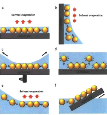
Fig. 3-1 Several microsphere lithography strategies

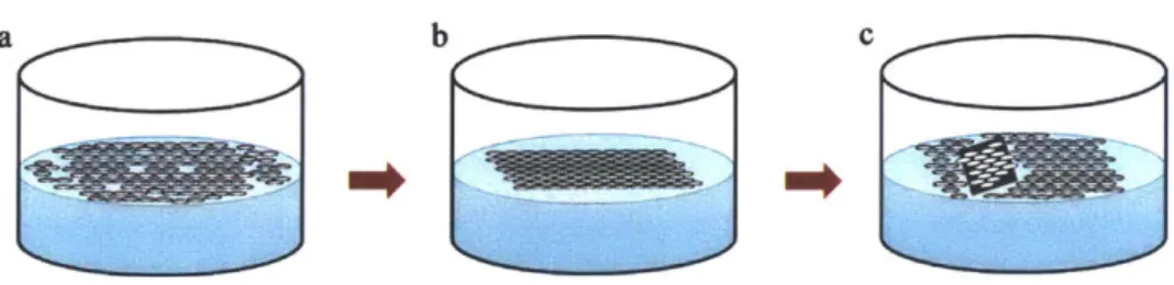
Fig. 3-2 Process of the microsphere lithography of polystyrene particles

Fig. 3-3 SEM images of 2D polystyrene patterns

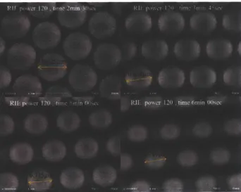
Fig. 3-4 SEM images of polystyrene beads etched by oxygen

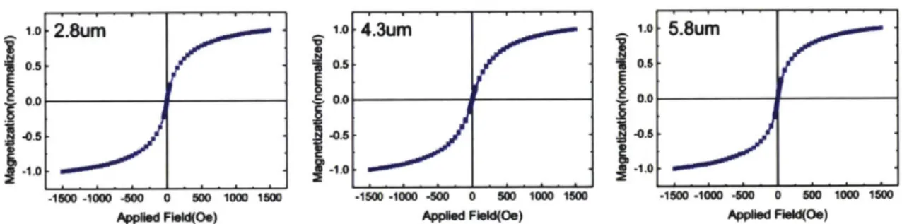
Fig. 3-5 Hysteresis loop of each superparamagnetic bead

Fig. 3-6 Sample preparation with suspension of magnetic beads

Fig. 3-7 Customized vector electromagnet with magnetic base and poles

Fig. 4-1 Schematic of superparamagnetic bead motion experiments

Fig. 4-2 Velocity as a function of frequency and critical frequency as a function of fields

(12)

Fig. 4-5 Optical microscopy images showing a series of SPB movement snapshots

Fig. 4-6 Remanent spin states in a unit cell from micro-magnetic simulation

Fig. 4-7 MFM images of DW structures

Fig. 4-8 Relaxed magnetization configuration and magnetostatic potential energy landscape

Fig. 4-9 SEM images for Co antidot arrays and velocity as a function of frequency

Fig. 4-10 Critical threshold of both Hip and Hoop for both 0 = 0 0 and 0 = 450

Fig. 4-11 Velocity as a function of frequency at SPB diameter of 2.8 jim on each symmetry lattice

Fig. 4-12 Threshold behavior of both Hip and Hoop with 2.8 pim for each lattice antidot array

Fig. 4-13 Velocity as a function of frequency at SPB diameter of 2.8 pim and 4.3 jm

Fig. 4-14 Critical threshold of Hip and Hoop for both 2.8 pim and 4.3 pim on the square antidot array

Fig. 4-15 Magnetization configuration and potential energy landscape of various diameter of SPBs

Fig. 5-1 Depth of the magnetostatic potential wells along the diameter-to-periodicity ratio

Fig. 5-2 Velocity as a function of frequency with an SPBs 2.8 pim

Fig. 5-3 Critical frequency as a function of both Hip and Hoop

Fig. 5-4 Relaxed magnetization configuration and Magnetostatic potential energy surfaces

Fig. 5-5 Critical frequency as a function of field and series of images of bead movement

Fig. 6-1 Hysteresis loop of continuous samples with Co (t nm)/Pt (5 nm)

Fig. 6-2 Hysteresis loops of continuous films with [Co(lnm)/Pt (t nm)]5

Fig. 6-3 Hysteresis loops of antidot arrays with [Co (Inm)/Pt (t nm)]5

Fig. 6-4 Velocity behavior on antidot-array with PMA and in-plane magnetic anisotropy

Fig. 6-5 Graph of velocity on the square lattice with PMA

(13)

Fig. 6-8 Magnetostatic potential well for square lattice and cross-section of the wells

Fig. 6-9 Relaxed magnetization configuration and magnetostatic potential well of hexagonal lattice Fig. 6-10 Optical microscopy images showing a series SPB movement snapshots

Appendix Fig. I SPB movements snapshot on continuous film with in-plane anisotropy Appendix Fig. 2 SPB movements on square symmetry antidot arrays with in-plane anisotropy Appendix Fig. 3 SPB movements on hexagonal symmetry antidot arrays with in-plane anisotropy Appendix Fig. 4 SPB movements snapshot on continuous film with out-of-plane anisotropy Appendix Fig. 5 SPB movements on square symmetry antidot arrays with out-of-plane anisotropy Appendix Fig. 6 SPB movements on hexagonal symmetry antidot arrays with out-of-plane anisotropy

(14)

List of Frequently Used Symbols

a Damping parameter Br Residual induction Bs Saturation induction Co Cobalt DW Domain wall d Diameter of the SPBs

FACS Fluorescence-activated cell-sorting

f

rotational frequency

fc

Critical frequency

Hc Coercivity

Heff total effective field

Hip Out-of-plane field Hoop In-plane field

hcp hexagonal-close-packed HMDS hexamethyldisilzane

K uniaxial magnetic anisotropy constant

Keff Effective anisotropy constant

y Gyromagnetic ratio

M Volumetric magnetization MFM Magnetic force microscope

(15)

magnetostatic energy

Ms Saturation magnetization Mr/Ms Squareness

ncp monolayers and non-close-packed

OOMMF Object-oriented micro-magnetic framework PDMS Polydimethylisiloxane

p distance from center to center or periodicity PMA Perpendicular magnetic anisotropy

RIE Reactive ion etching

SEM Scanning electron microscope SPB Superparamagnetic bead SPBs Superparamagnetic beads TN Neel temperature TB Blocking temperature Tm Measurement time v velocity of SPBs

Vm volume of the SPBs or particle VSM Vibrating sample magnetometer

(16)

(17)

Chapter

1 Introduction

In this chapter, we motivate the importance of studying the interaction between superparamagnetic beads (SPBs) and periodic magnetic patterns for the dynamics of SPBs. Then, we briefly review the outline of the thesis.

1.1 Motivation

Micrometer- or nanometer- sized devices for medical or biological applications have been widely studied during recent decades. The goal of most such research is to create fast, cheap, sensitive, and high-throughput platforms, and these are called "lab-on-a-chip" technologies in analysis systems.

The key technologies of lab-on-a-chip are transporting biological species across the surface of the chip, which can be controlled by simple or remote methods. Surface-functionalized micrometer- or nanometer- sized beads are popular ways to transport biological species. Taking advantage of the small diameter of the beads, options for surface modification, and actuation modes. In fluidic environments, beads with biological matter can be transported, controlled, and manipulated. Therefore, techniques based on beads open the possibility of future biological applications such as drug delivery, hyperthermia, and MRI enhancement, which can be based on acoustofluidics, ~- optical images,9-'5 hydrodynamics,16-21 thermophoresis, electrophoresis,23-26 dielectrophoresis,27 31 and magnetic force.3246

(18)

Magnetic systems inducing bead motion have many advantages. Magnetic particles or

entities can be manipulated using discrete permanent magnets or electromagnets, independent of

normal microfluidic or biological processes.47-48 Furthermore, such magnetic systems do not need

complex experimental components such as micro channels, electrical connections, pumps for fluid

flow, reservoir chambers.49 Localized heating is known to cause problems in lab-on-a-chip devices,

but magnetic fields do not degrade biological entities and are thermally stabilized,5 0 5' unlike

electric fields.12-13

Furthermore, magnetically activated cell-sorting can be possible simultaneously,

offering high throughput, while fluorescence-activated cell-sorting (FACS) which is a sequential

43

process

In recent decades, nano- or microsized SPBs with functionalized surfaces have been widely

applied in biological analysis applications using transport, switching, mixing, separation, and

detection. Initial on-chip bead manipulation studies were based on bulky permanent magnets in

fluidic microchannels5 4 59. The simplicity of this system is attractive, but the formation of SPB

aggregation leads to attenuated optical signals and mechanically damages the biological cells.

Electromagnets that are located in microchannel have also been used for magnetic manipulation.

In these structures, the magnetic field gradient usually produce 104-105 Tm-1 in a local regime,

which sufficiently supports the transport of SPBs. Several designs, including current-carrying

wires6 0-62, high aspect ratio trenches63-64, and several arrays of coiled wire65 have been developed

to precisely control SPBs. However, these electromagnets within microchannel have limitations in

terms of the complexity of fabrication, a nonlinear position dependence of the force profile, and

heating problems from the large number of electromagnets.

(19)

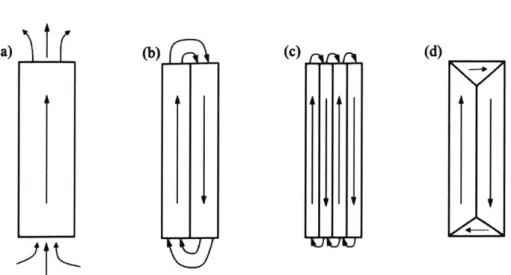
wall magnetophoretic transport, and nonlinear magnetophoresis. In the first, the SPBs are transported on de-magnetizable structures such as Nio.8Feo.266. By applying a rotating magnetic

field in the xy plane, the soft micro-magnets are easily demagnetized and the magnetizations of micro-magnet elements are changed along each direction of the magnetic field. The SPBs follow the net magnetization of the magnetic structure and are transported along the perimeter of the micro-magnet elements such as ellipses 66-68, connected disks or half-disks69-7 3_{, triangles}4 9_'74_{, and}

other complex configurations 75. In the case of symmetric elements, such as disks, H_ is required to move the SPBs from one element to another; otherwise, the SPBs exhibit a closed orbit around the

element.

In the second mechanism, using the stray field from the domain walls in thin films has been

76-79

used to control the movement of SPBs. For example, in a thin film of Y2.sBio.sFes-GaqO2

-magnetic domains are configured in a stripe-pattern with periodicity A, and the travelling distance of SPBs on this film is A for a rotational period. In continuous films, applying a high-frequency magnetic field with pulses can create "bubble" domains7 8_{'80-81, which trap the SPBs. The transport}

of SPBs is controlled through the magnitude of the normal field component H. Furthermore, the transport of beads on patterned zigzag nanowire has been widely studied with head-head (HH) and tail-tail (TT) domains at the vertices of the wire82-87. The domain walls with SPBs were shifted by applying Hy and H- magnetic fields, the latter of which controls the depth of the potential well. The geometry of domain wall conduits also includes ring, square, or rectilinear conduits, where the SPBs can be smoothly transported using an Hy field33

,34,8 4_-8 5_,88_-90

The final mechanism for SPB transport is based on nonlinear magnetophoresis using hard micro-magnet arrays. A traveling magnetic field wave, which results from the superposition of an

(20)

SPBs36_-37_,91_-92

. The velocity of SPBs increases linearly with the frequency of the rotating field until a critical frequency (ae), beyond which the velocity rapidly drop-off and the SPBs locally oscillate.

Using the dependency on the a), multiplex separation is possible for a heterogeneous sample.

However, the separation efficiency is limited by the sharpness in the transition from "mobile" to

"immobile" beads, which is influenced by the ratio of the diameter of SPBs and the periodicity of

patterns.

In this thesis, for the first time, the dynamics of SPB transport on antidot arrays is fully

investigated and characterized. Whereas previous studies have focused on the critical frequency to

sort the SPBs, we explore the dynamics of SPBs and elucidate the interaction between the SPBs

and various magnetic patterns. Through several micro-magnet structures with different magnetic

anisotropy and geometry, we show different behaviors of SPB transport. Thus, we not only

demonstrate the controlling parameters such as the critical frequency as well as the threshold

behavior in a magnetic field, but also show magnetic potential distribution to play a key role to

understand the dynamics of SPBs. Finally, with this knowledge, we design a multilayer structure

(21)

(22)

1.2 Thesis outline

Given the advantages of micro-magnetic lab-on-a-chip technologies, the aim of this thesis is to develop several parameters to precisely control SPB transport and establish micro-magnetic arrays to enhance the dynamics of SPBs, including capture, transport, and sorting. Accordingly, the thesis is organized as follows:

- Chapter 2 discusses the physical phenomena and fundamental concepts needed to support this inquiry: magnetic energy, magnetic anisotropy, domain walls, and superparamagnetism.

- Chapter 3 explains the simulation and fabrication methods that are used in this thesis.

- Chapter 4 demonstrates that the dynamics of the SPBs can be controlled by the critical frequency as well as the threshold behavior in magnetic fields. These controlling parameters depend on the patterns of the magnetic configurations or lattice geometry.

- Chapter 5 reveals that bead sorting based on these controlling parameters can be achieved throughout the entire range of micro-magnet arrays. We introduce self-assembly methods, which are simple and cheap ways to produce small-scale micro-magnet arrays.

- Chapter 6 demonstrates the enhanced dynamics of SPB motions on the perpendicular magnetic anisotropy substrate and the widened scope of the capability of magnetic fields to transport SPBs. We also explain the different transport of SPBs on various lattice geometries through simulation results.

(23)

Chapter 2 Background

In this chapter, we discuss the fundamental phenomena relevant to developing a magnetic lab-on-a-chip. First, we describe the details of the magnetic concept, including magnetic anisotropy and superparamagnetic beads. After that, we will discuss magnetotransport, which will become important in later chapters for understanding the mechanism of bead transport.

2.1 Basic concepts

2.1.1 M-H curves

When a magnetic field of strength H is applied to a material, the response of the material is called magnetic induction B. All the individual atomic moments in the materials will contribute to the response, and the relation between B and H is proportional to the material properties. Generally, the equation relating B and H is given by:

B = pO(H + M) (1)

where yo is the permeability of free space, and M is magnetization, defined as the magnetic moment per unit volume M= m/V, where m is the magnetic moment on a volume V of the material.

(24)

Furthermore, the magnetic properties of materials are defined not only by the magnetization, but also by the magnetic susceptibility, which varies with the applied magnetic field. The magnetic susceptibility is the ratio of M to H, where the magnetization induced in a material by H93:

M

X = - (2)

H

where X is dimensionless and both M and H are expressed in Am~. Most materials can be classified either as paramagnets, for which X falls in the range 10-6 -10-, or diamagnets, where X is in the range -10-6 to -10 .However, some materials exhibit ordered magnetic states without applying a field; these materials are classified as ferromagnets, ferrimagnets, or antiferromagnets. The coupling interaction between the electrons within the materials leads to spontaneous magnetization and exhibits different ordering based on the nature of the coupling interaction. The susceptibility in ordered material depends on temperature as well as on H. Therefore, each material exhibits the characteristic sigmoidal shape of the M-H curves when a large value of H is applied. In ferromagnet and ferrimagnet materials, the M-H curves show hysteresis, which is an irreversible magnetization process due to the pinning of magnetic domain walls at grain boundaries or impurities as well as to intrinsic properties such as the crystalline magnetic anisotropy.

Figure 2-1 describes the typical hysteresis loop for the ferri- or ferromagnet, plotted B versus H. The loop started at the original, unmagnetized state, and B follows the curve from 0 to B,, which is the saturation induction. Here, we note that although the magnetization is constant after saturation, B continually increases due to B = po(H + M). When H is reduced to zero after saturation, B reduces from B, to B, (remanence induction), and the reversal field required to reduce

(25)

a

0 H

Figure 2-1 Hysteresis loop for ferrimagnet or ferrromagnet. From Nicola A. Spaldin, Magnetic Materials:

Fundamentals and Device Applications, (Cambridge University Press, 2003)

2.1.2 Magnetic energy

In this section we discuss several magnetic energy terms used in micro-magnetics, which describe magnetic behavior at sub-micrometer length scales. To determine the spatial distribution of the magnetization M at equilibrium, the magnetic energy, including exchange, anisotropy, Zeeman, and magnetostatic energy, should be minimized.

The exchange energy is based on the quantum-mechanical exchange interaction and is defined as94_:

Eex = A 2 (3)

(ax)

where A ==s2a2j₁₁N'/2 is called the exchange stiffness constant, a is lattice constant, ;j; is

(26)

divergence a- and exchange stiffness A. Therefore, exchange energy tends to keep adjacent

ax

magnetic moments aligned in parallel or antiparallel, producing antiferromagnetism, ferrimagnetism, and ferromagnetism. For example, it is responsible for ferromagnetic behavior, where the magnetization retains a parallel direction at saturation.

Anisotropy energy represents the directionality dependence for spins to align along a certain direction. Considering the magnetocrystalline anisotropy in the uniaxial case, this is given

94

as

Ua = Kansin2n9 (4)

n

where Ua is the uniaxial crystal anisotropy energy density, Kun is the uniaxial anisotropy constant, and 0 is the angle between the spin and the preferred direction.

The Zeeman energy is due to the misalignment of the magnetization in an applied field, and is described as94:

UH = -POMs -HO = -pOMHOcosO (5)

where 6 is the angle between the magnetization M and field H. This energy decreases as the angle 0 decreases.

Finally, the magnetostatic energy is created by the magnetic sample itself and arises mainly from having a discontinuity in the normal component of magnetization across an interface. The energy results from the interaction between the spin and the dipolar demagnetization field, which is the field inside the sample. It points along the opposite direction to the magnetization. Therefore, the magnetostatic energy is an anisotropic energy that depends strongly on the shape of the samples. The magnetostatic energy is defined

(27)

as94-Ums = -IOM - Hi = -pOMsH1cos (6)

where M, is the saturation magnetization of the material, and the internal field Hi = Happl+Hd is a function of the externally applied field Happi and the dipolar demagnetizing field Hd. Therefore, the

demagnetization field contributes to decreasing the magnetostatic energy. In addition, as the angle 0 between the direction of magnetization and the direction of internal field increases, the

magnetostatic energy also increases.

Here, we note that the exchange and magnetostatic energy contribute in opposite ways, where the exchange energy favors parallel spin alignments, and the magnetostatic energy prefer antiparallel alignment. Therefore, the extent / over which energy dominates is characterized by the exchange length, and it varies with the type of domain wall95_{. For hard materials with large} crystalline anisotropy, the typical domain wall is the Bloch type. In that case the width of the Bloch wall is 6B = w /A/KU, where A is the exchange constant in J/m and Ku is the uniaxial anisotropy constant in J/m3_{. The magnetocrystalline exchange length 1 is defined as A/Ku in the hard}

materials; while in very thin films, composed of magnetically soft materials, A Neel wall is the typical structure. The width of these walls is around 3 A/Kd, where Kd = poM,/2 and the

magnetostatic exchange length is:

lex = [2A/(otMS) (7)

In this case, the exchange interaction is dominant when 1 < ex while the magnetostatic interaction is dominant when l> Le.

(28)

2.1.3 Magnetic anisotropy

Magnetic anisotropy is the preference for the magnetization to lie in a certain direction in the samples. Magnetic anisotropy has several origins including shape anisotropy, magnetocrystalline anisotropy, magnetoelastic anisotropy, and exchange anisotropy.

Magnetocrystalline anisotropy is a force which hold the magnetization in certain crystallographic directions in a crystal 96. The crystal anisotropy energy in a cubic lattice, which is the energy needed to align magnetization along a non-easy direction, can be expressed as:

E= K + K1(aa+ a2a2 + a2a2) + K2(a2 a2a2) + (8)

where KO, K1, K2,.. are the constants for particular materials and a,, a2, a3 are the cosines of the angles between Ms and crystal axes. Usually Ko is ignored because it is not changed by the angle, and the values of both K1 and K2 determine the direction of easy and hard magnetization. For

hexagonal crystals, all directions in the basal planes are hard axes and the magnetocrystalline anisotropy energy depends on only a single angle, 0, between the Ms vector and the c axis. In this case, the anisotropy can be described as:

E = K' + K1cos 20 + Kicos4_{0 +} ₌ _{KO + K}

1sin2 + K2sinO + (9)

The physical origin of magnetocrystalline anisotropy is spin-orbit coupling. When the external field tries to reorient the spin of an electron, then the orbit of that electron also tends to be reoriented. However, the orbit is also strongly coupled to the lattice, so energy is required to overcome the resistance. This energy can be measured by several methods, including torque curves, torsion pendulum, magnetization curves, and magnetic resonance.

(29)

The shape anisotropy is dependent upon the shape of the sample. As mentioned in Section 2.1.2, the demagnetizing field along a short axis is stronger than along a long axis. When a field is applied along a short axis, the same field is produced inside the specimen. Therefore, the shape itself can be a source of magnetic anisotropy. Considering a prolate spheroid with semi-major axis c and semi-minor axes a of equal length, as shown in Figure 2-2, the magnetostatic energy is defined as96:

1

Ems = -[(Mcose)2N, + (Msin6)2 _Na] ₍₁₀₎ 2

where Nc and Na are demagnetizing coefficients along c and a, respectively. Substituting cos2₆

1 - sin2 _{, then the above equation is expressed as:}

1 1

Ems = 1 M 2

Nc + (N _ N)M2_sin2

O (11)

2 2

In this magnetostatic energy expression, it has the same form as uniaxial crystal anisotropy energy, an angle-dependent term, and the long axis of the sample plays the same role as the easy axis of the crystal. Thus, the shape-anisotropy constant K, is given by:

1

Ks = -(Na - NC)M2 ₍₁₂₎

2

The magnetic moment is easily aligned along the c-axis and is hardly aligned with any axis normal to c. For the spherical shape, the shape anisotropy disappears (Ks=0) because c equals a and Na = Nc.

(30)

M

Figure 2-2 Prolate ellipsoid. From B. D. Cullity and C. D. Graham, Introduction to Magnetic Materials, (Institute of Electrical and Electronics Engineers) (1991)

The magnetoelastic energy is based on the magneto-elastic effect, which comes from spin-orbit interactions. The moment of spin is coupled with the lattice through spin-orbital electrons. If the lattice is changed by strain, then the distance between the magnetic moments is also altered. Therefore, the interaction energies are changed and it produces magneto-elastic anisotropy. This is correlated to the phenomenon where the permeability or susceptibility of a material is changed when applying a stress on the material. Generally, without a stress M is controlled by magnetocrystalline anisotropy as characterized by the first anisotropy constant Ki. However, when a stress is applied, the direction of M is controlled by both K and a. Therefore, the energy in a cubic crystal, which depends on the direction of M, is defined as:

E = K1(aai + aa3 + a )(a y + a y2 + a y) (13)

- 3Ajjja(a₁a₂Y₁Y2 + a2a3Y1Y2 + a2a3Y2Y3 + a3a1y3y1)

where a1, a2, a3 are the direction cosines of M and yi, Y2, Y3 are the direction cosines of the

stress a. The first term of the equation is the magnetocrystalline anisotropy and next two terms are called the magnetoelastic energy. The final direction of M is that which minimize E and the direction is determined by various parameters such as K1, /10, l,, and a for any given stress

(31)

direction yi, Y2, Y3- In the elastically isotropic materials with isotropic magnetistrictions (A100=

Al, = Asi), the magnetoelastic energy is:

3 3

Eme = Asi-cosA2 _ .=sin2

0 (14)

2 2

where & is the angle between M and a.

Finally, exchange anisotropy is observed at the interface between an antiferromagnetic

material and a ferromagnetic material, where an exchange coupling is magnified. The typical

features of exchange anisotropy are a shifted loop and high-field rotational hysteresis, and these

are observed in multilayer structures and alloys. For example, when a strong field is applied to

Co-CoO particles at 20'C (the Ndel temperature, TN, of CoO is about 20'C) the cobalt is magnetically

saturated but the oxide is paramagnetic. However, the spins of the first layer of Co ions in the

oxide are forced to be parallel to the adjacent cobalt atom due to the positive exchange force

between the spins of adjacent Co atoms. When the particle is cooled below TN with a field, the

antiferromagnetic ordering is caused in the oxide, and the spin arrangement still persists at the

interface. If the field is applied in the opposite direction, then the spin in the Co will reverse, and

the spins of the oxide are forced to reverse due to the exchange coupling at the interface. However,

this rotation is resisted by the crystal anisotropy of the antiferromagnet, so partial rotations of a

few spins appear at the interface. This anisotropy usually displays unidirectional anisotropy, so the

anisotropy energy is proportional to the first power of the cosine rather than the square of the

cosine

(32)

where K is the anisotropy constant and 0 is the angle between M, and the direction of the cooling field. Thus, the requirements for establishment of exchange anisotropy are field-cooling through

TN, contact between ferromagnetic and antiferromagnetic materials, and strong crystal anisotropy

in the antiferromagnet.

2.1.4 Magnetic Domain walls

97

The concept of a magnetic domain introduced by Pierre-Ernest Weiss in 1906. It were first experimentally observed in silicon-iron single crystal was by H. J. Williams, R. M. Bozorth, and W. Shockley in 1949. 98 Since this observation, domain theory is used to describe many magnetization processes. A domain indicates the interface in which the spontaneous magnetization has different directions, so the magnetizations are changed from one easy crystallographic direction to between domains99. This effect can be understood from an energetic perspective. In Figure 2-3 (a), the free magnetic poles at the edge of the sample are relatively strong, resulting in a large magnetostatic energy. By introducing the 1800 DW in Figure 2-3 (b), the magnetization of each domain points in different direction, and the magnetostatic energy is reduced. Although

introducing DWs costs energy due to the exchange interaction, their presence is energetically favored in many magnetic systems.

(33)

(a) (b) (c) (d)

j1

Figure 2-3 Magnetostatic energy and domain formation (a) magnetostatic (MS) energy of the single domain state, (b) Introduction of 1800 domain walls to reduce MS energy, but increasing the wall energy, (c) smaller MS energy, but higher wall energy, (d) 900 closure domains eliminate MS energy, but cause elastic energy due to the strain incompatibility and increasing the anisotropy energy. From O'Handley, R.C. Modern magnetic materials: principles and applications. (John Wiley & Sons, Inc., 2000).

In a microscale structure, wide DWs become energetically unfavorable, as they serve as a transition area between different magnetizations. The internal structure of DWs are generally dependent on the size, structure and material parameters of the sample. However, there are two competing energy terms which are involved in spin orientations in a DW: anisotropy energy and exchange energy. As shown in the Figure 2-4, where the spin orientation in the thin film and the term from magnetostatic energy is neglected, the exchange energy prefers a parallel alignment of spin, which minimizes the angle difference between the spins. On the other hand, the anisotropy energy prefers an alignment of magnetization along an easy axis such as x axis, minimizing the number of spins pointing along an unfavorable hard axis. Therefore, the exchange energy prefers gradually changing the spin direction in DWs over a large length scale, whereas the anisotropy energy tends to reduce the DW width to minimize the number of spins which align along the hard

(34)

N

Gex + = ISJaSn 2 2 + Ksin2OdG (15)

i-1

where J is the exchange anisotropy constant, S is the electron spin, N is the number of spins within the DW, and 0 is the angle between the nearest neighbor spins, K is anisotropy constant.

94

Considering the simple DW case, the above equation can be written as

Uex + 0ant ~S 2 2 + KuNa (16)

where a is the atomic constant, angle approximately &ij ~wT/N, and integral approximation for simplicity. The above equation has dependency on N, which is directly correlated to the width of the DW. It is minimized for No = US2 2_/Ka3₎

1/2 and the width of the DW is No a

i(A/K,)1/2, where A is the exchange stiffness constant A = JS2/a. For example, the thickness of

a DW in soft materials with small anisotropy is approximately 0.2 pm, whereas the thickness of a DW in hard materials with high-anisotropy is approximately 10 nm.

(a)Anisotropyenergy minimintion

- x axis (b) Exchange energy minimizaton

(35)

The most common type of 180* DW is a Bloch wall, where the magnetization rotates in the plane parallel to the plane of the DW. The other DW type is a I4eel wall, where the magnetization rotates in the plane perpendicular to the plane of the DW. The DW energy densities for these DWs have different due to the thickness of the thin film. The Bloch wall energy increases with decreasing film thickness because of increasing magnetostatic energy at the charged surface. However, the Neel wall energy density decreases with decreasing film thickness because the amount of surface is also reduced, and the Neel wall is usually stable in magnetic thin films below 50 or 60 nm thickness. In this thesis, all the in-plane magnetic anisotropy samples (IMA) exhibit

several kinds of DW structures due to the antidot patterns. Furthermore, the remnant magnet configurations have dependency on the symmetry of the pattern, the periodicity of pattern, and the diameter of the hole, as shown in Figure 4-6.

+

(a) Bloch wall (b) Neel wall

Figure 2-5 Two different types of domain wall: (a) Bloch wall, with charged surfaces on the external surfaces of the sample and (b) Neel wall with charged surfaces internal to the sample. From O'Handley, R.C. Modern magnetic materials: principles and applications. (John Wiley & Sons, Inc., 2000).

(36)

2.1.5 Perpendicular magnetic anisotropy

The presence of perpendicular magnetic anisotropy (PMA) is a complicated phenomenon because magnetostatic potential energy generally favors an in-plane anisotropy (IMA) according to the conventional theory of magnetic thin films. As mentioned in Section 2.1.3 magnetic anisotropy, the magnetization of a thin film prefers the direction that can reduce the demagnetization fields. If the magnetization of a thin film is magnetized along the z axis (out-of-plane), then the magnetic free poles generate a large demagnetization field, which is unfavorable. Therefore, to prevent a large demagnetization field, the magnetization of a thin film tends to align in the plane of the material. However, with the introduction of new concepts such as spin-orbit interaction, the easy axis of a thin film can be parallel to the z-axis when an ultra-thin ferromagnetic layer is embedded between nonmagnetic materials such as Pt and Pd' 0 0_-103 _{or a capping oxide such}

as MgO10 4 or Gd2O, 105.

PMA can be explained by a strong interfacial interaction, and it can be described by an effective anisotropy constant' 06-17 in Co/Pt multilayers:

2K

Kef = 2 + K (17)

tco

where tco is the thickness of an individual Co layer, Ks is the anisotropy originating from the interface per unit area, Kv = K, - O.5pOM,2 is the volume contribution of Co, including

magnetocrystalline, magnetoelastic anisotropies, and a negative shape anisotropy term. Thus, the anisotropy of materials is determined through the competition between the magnetostatic energy minimization and energy reduction by the spin-orbit coupling. By decreasing the thickness of Co

(37)

layer, the effective anisotropy changes from negative to positive, indicating a transition from in-plane anisotropy (Keff < 0) to out-of-in-plane anisotropy (Keff > 0) .

The materials with PMA have a great deal of advantages compared to the material with IMA. First, the average anisotropy energy of PMA materials is much larger than that of in-plane materials. As shown in Section 2.1.3, the width of a domain wall is determined by two competing energies: the exchange energy and the anisotropy energy. When increasing the anisotropy energy, the width of a DW becomes narrower, so DWs in PMA materials are narrower than in IMA materials. For example, the width of DWs in a PMA material is around 1~10 nm; while that of DWs in an in-plane material is approximately 100nm94. Furthermore, thermal instability, which results in the curling of magnetization and is frequently observed at the edge of in-plane materials, is not exhibited in PMA materials' .4-1 Consequently, these structures have been widely studied and have attracted a great deal of interest in high density magnetic recording research.'1 6

(38)

2.2 Superparamagnetic beads

Lab-on-a-chip or biomedical applications based on microfluidic systems generally use magnetic nano- or microparticles which can be easily manipulated using a permanent magnet or electromagnets, independent from normal microfluidic or biological processes ..-. 9. The size of these magnetic particles varies from several microns in diameter down to tens of nanometers". Superparamagnetic behavior is dependent on the size of particle, such that larger microscale magnetic particles cannot exhibit superparamagnetism. However, micro-sized particles can be designed to have superparamagnetism through composition. Generally, these beads or particles consist of many separated small, superparamagnetic grains of iron oxide (magnetite Fe304 or

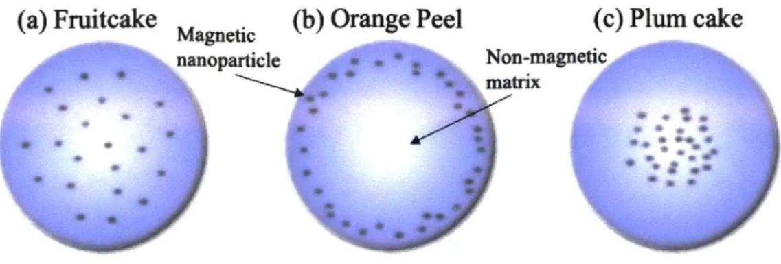
maghemite y-Fe2O3), embedded in a polymer matrix such as polystyrene120. Recently, three types

of embedding for the paramagnetic micro-sized beads have been reported by Thanh'21: "fruitcake" (the nanoparticles are uniformly distributed in the matrix), "orange peel" (the nanoparticles are located on the surface of the bead), and "plum cake" (the nanoparticles are concentered in the center of matrix). Figure 2-6 shows these three types of micro-sized superparamagnetic beads. The matrix also serves as a separator medium to reduce inter-particle interaction and prevents the loss of superparamagnetism. The surface of superparamagnetic beads is coated to stabilize the beads in solution and render them non-toxic and biocompatible. For example, superparamagnetic particle used in biomedical applications should be water-dispersible. Thus they usually feature a hydrophilic surface coating such as a carboxylate-functionalized group.

(39)

(a) Fruitcake (b) Orange Peel (c) Plum cake

nanoparticle Non-magnetic

matrix

Figure 2-6 Several types of superparamagnetic microbead. From Ruffert, C. Magnetic bead-magic bullet, Micromachines, 7, 21 (2016)

Nowadays, a variety of magnetic beads are used for different applications and they are commercially available: Dynabeads* magnetic beads provided by Invitrogen, BcMagTM by Bioclone Inc., ProMagTM and BioMag* from Bangslabs, SupraMagTm _{by Polymicrosheres Inc.,}

TurboBeads* by Turbobeads Lic., and SPHEROTM Polystyrene Magnetic Particles by Spherotech. These superparamagnetic beads are used in binding, purification, and magnetic separation of biomolecules such as proteins, cells, DNA fragments, and antibodies, because the size of beads are comparable to those of cells (10-100 pm), proteins (5-50 nm) and small bacteria (20-450 nm). In addition, these superparamagnetic beads which can be manipulated by a magnetic field do not maintain their magnetization and decompose into particles after removing the magnetic field. As mentioned before, unlike electrical manipulation, the magnetic interaction rarely affects the

122

sensitive parameters biological applications such as pH, ionic concentration, and temperature. Furthermore, biological systems usually have little magnetic susceptibility, which results both in high selectivity and non-interference of magnetic fields. Therefore, superparamagnetic beads have potential for use in immunoassays, cell manipulation and cellular-specific targeting, DNA

(40)

extraction 12 3_{, magnetic resonance imaging'} 2 4_{, targeted medication}1 25_{, and hyperthermia}

therapiesc .

Given the advantages of superparamagnetic beads, the beads are widely studied and used in lab-on-a-chip applications. In the following section, we discuss what the superparamagnetism is and several forces that act on magnetic particles.

2.2.1 Superparamagnetism

Superparamagnetism is observed in small ferromagnetic particles on the order of tens of nanometers or less due to fundamental size-effects. In nano-particles, reduced energy from a multi-domain configuration is no longer favorable, so the small particles generally consist of single domain structure with magnetization reversal occurring via coherent spin rotation rather than through domain expansion via domain wall propagation.

The typical radius below which a spherical nano-particle will be single domain is given by94,12 7.

Rsd - 6 (18)

where A, the exchange stiffness, is a measure for the critical temperature for magnetic ordering of the material, K is the magnetic anisotropy of the particle, Io is the permeability of free space, and M, is the saturation magnetization. For most magnetic materials, the size limit for superparamagnetism is in the range of 10-100nm.

(41)

Since the first research done by Neel 2 8_{, Brown'}_29,_{and Aharoni" on uniaxial magnetic}

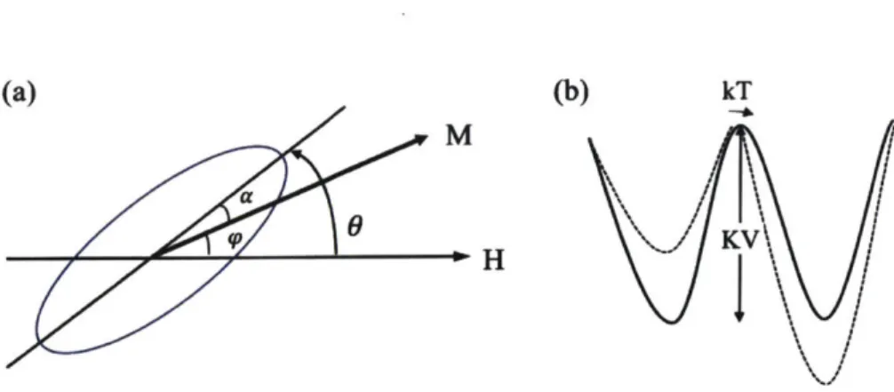
nanoparticles, superparamagnetic relaxation process has been well studied. Generally, a particle with uniaxial anisotropy is designed as a prolated spheroid with the easy axis of magnetization along the major axis. As shown in Figure 2-7, the magnetic anisotropy energy is given by127

Eani(a) = -KVcos 2_za ₍₁₉₎

where a is the angle between the direction of magnetization Mand the easy axis, V is the volume of the particle, and K is the uniaxial magnetic anisotropy constant. Figure 2-7 (b) represents the magnetic anisotropy energy as a function of the angle, a, where two minima of energy are located at a = 0 and wT, separated by an energy barrier KV. Without an external field, the magnetic moment of a particle has equal probability to arrange along either direction of the easy axis. Reversal between the two minima can be achieved when the thermal energy is larger than energy barrier (kBT > KV). According to the Neel-Brown theory12 8

-129_{, the relaxation time}

T of the net magnetization of the particle under an activation law is:

T

=

Toexp

(IT)

(20)

where AE is the energy barrier to moment reversal, and kBT is the thermal energy. For the non-interacting particles, the pre-exponential factor -ro is of the order 10' -1022s and only weakly dependent on the temperature. For the energy barrier AE , this term is correlated to the magnetocrystalline anisotropy, shape anisotropy, strain anisotropy, and exchange anisotropy.

(42)

(a)(b) kT M

aH

Figure 2-7 (a) Schematic of a prolate spheroid depicting a nanoparticle with uniaxial magnetic anisotropy in the presence of an external magnetic field Hat an angle 0 relative to the direction of the anisotropy axis. Angles a, p give the orientation the magnetization of the particle, M, relative to the anisotropy axis and the magnetic field, respectively. (b) Magnetic potential energy as a function of angle a, in the absence of an applied field, solid line, and in the presence of an applied field along the anisotropy axis, dash line. The minima occur at a = 0, 1T. From Papaefthymiou, G. C. (2009). Nanoparticle magnetism. Nano Today, 4(5),

438-447. https://doi.org/l 0.101 6/i.nantod.2009.08.006

Thermally activated flipping of the net moment direction can be observed when AE is

comparable to kBT. For example, at room temperature and for the small particles, the AE of

moment reversal is equivalent to the thermal energy so the time-averaged magnetization of the

particle is measured as zero. Therefore, the barrier AE, which is proportional to the particle

anisotropy and volume, is an important factor to develop the superparamagnetism. In addition, the

observation of superparamagnetism is also dependent on the measurement time Tm of the

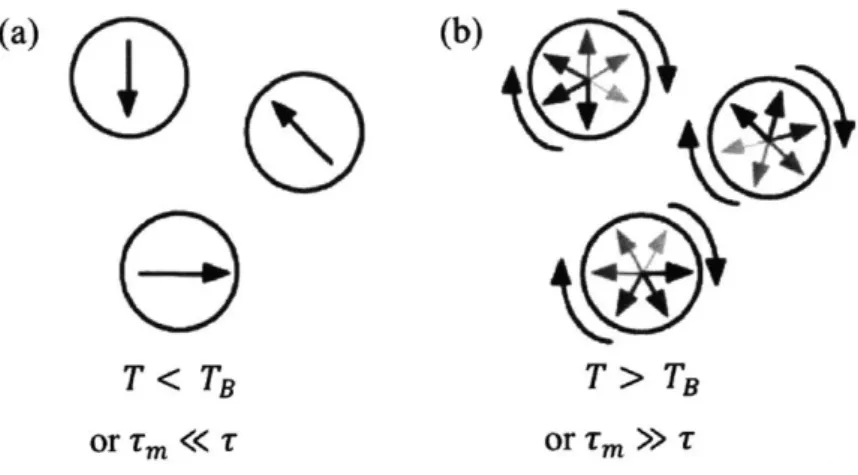
experimental technique. As shown in the Figure 2-8, if the relaxation time is much larger than the

measurement time (T <Tm), then the flipping is fast relative to the experimental time and the

time-average moment of particle is measured as zero. This state is the superparamagnetic state. If

the relaxation time is much smaller than measurement time (T > Tm), however, then reversal is slow and a well-defined state can be observed. This is called a 'blocked' state of system. The

(43)

(a)

0

T<TB or Tm

«

T

0

(b) T>TB or Tm >

Figure 2-8 The circles depict three magnetic nanoparticles, and the arrows represent the net magnetization direction in those particles. (a) The measurement time Tm is much smaller than the relaxation time. A well-defined state can be observed (quasi-static state). (b) The measurement time Tm is much larger than the relaxation time, then a time-averaged net moment of zero will be observed (superparamagnetic state). From Pankhurst, Q. a, Connolly, J., Jones, S. K., & Dobson, J. (2003). Applications of magnetic nanoparticles in biomedicine. Journal of Physics D: Applied Physics, 36(13), R167-R181. https://doi.org/10.1088/0022-3727/36/13/201

2.2.2 Force on a magnetic particle

In order to understand how a magnetic field can transport and manipulate magnetic beads,

it is important to quantify the magnetic field gradient, supporting the transport of the beads. While

a uniform magnetic force only exerts a torque on the beads, a field gradient can transport the beads.

From the consideration of a moment in a field B, then the magnetic potential energy is defined as:

(21)

U = -m-B

and the magnetic force is:

(44)

Fm = V(m - B) ~ (m - V)B

where the second part of the above equation is based on the magnetization m of the particle not varying in space (V - m = 0).

In the case of magnetic particles suspended in a weakly diamagnetic medium such as water, the total moment of the particle can be written m=VmM (where Vm is the volume of the particle and M is its volumetric magnetization.) The effective susceptibility of the particle is AX = Xm

-Xw, where Xmis the susceptibility of the magnetic particle, and Xw is the susceptibility of water. Thus,

B

H = - (24)

Mo where yo is the permeability of free space.

M = VmM =Vm XH (25)

Substituting these expressions and rewrite the expression for the force on a magnetic dipole in a magnetic field gradient gives:

V X

Fm = -(B - V)B (26)

Po

If we consider the magnetic particles that are constrained to move in the x direction, the x component of the force is defined as:

VX

a

Fm,x= Bx-+By +B (27)

Po ax ay Bx 27

Thus, both the magnitude of the magnetic field and the field gradient need to be large to have a (23)

(45)

2.2.3 Stokes drag force in viscous medium

In many applications, magnetic particles are separated in a liquid solution by Brownian fluctuation. Therefore, to transport the magnetic beads in a fluid it is necessary to consider the force exerted on the beads from the fluid. The inertial force and viscous force on the beads can be

133.

characterized by the Reynolds numbers, which is defined as

Re =pvL (28)

P

where p is the density of the fluid, v is a characteristic velocity of the fluid with respect to the object, L is a characteristic linear dimension, and p is the dynamic viscosity of the fluid. There are two types of flow: laminar and turbulent. Laminar flow occurs at low Reynolds numbers where viscous forces are dominant. While turbulent flows occurs at high Reynolds numbers where at high Reynolds numbers.

The hydrodynamic drag force, which is the result of the velocity difference between the magnetic particle and the liquid, is given by Stokes law34_:

Fd = 6rTirAv (29)

where rq is the viscosity of the medium surrounding the beads, r is the radius of bead, and Av is the difference between the magnetic particle and the liquid. From the Eq. (26) and Eq. (29), the maximum flow rate of the particle in a surrounding static liquid is47_:

2r2X(B - V)B 1

(46)

2r 2X VX

9= q= _ Vi (31)

9ij 6wtri

being the "magnetophoretic mobility" of the particles, which describe how magnetically manipulable the particle is.

2.2.4 Other forces on a magnetic particle

Other forces acting on the beads are electrostatic forces including van der Waals attraction and electrostatic repulsion, which lead to bead-bead interactions. These forces can be modified through surface coating. In addition, the DLVO interaction, which describe the aggregation of aqueous dispersions quantitatively, between the charged surface of beads and a liquid medium must also be considered, and the hydrophobic or hydrophilic characteristics of the bead can affect the dynamics of beads'35-3 7_{. However, these forces are complicated, and it is hard to represent} these forces as a general way in our model. Thus, these forces will not be considered in our simulation models, but they can be potential source of variation between simulation and experimental results.

(47)

2.2.5 Suprastructure formation

For the selective transport or separation of beads, agglomeration of the beads is not desired. The concentration of beads is usually kept low to prevent agglomeration and increase interbead distance. At high concentration, the beads tend to form supraparticle structures47 as described in Figure 2-9. Without an external magnetic field, the net magnetization of superparamagnetic beads is zero, and there is no magnetic interaction. By applying a magnetic field, a torque T acts on the

magnetic moment vectors M of the beads:

T = M x B (32)

Due to the torque T, the magnetic moments are aligned which leads to the development of a stray field. If the magnetic field is homogeneous, then the beads seldom assemble each other. However, if the interbead distance is small enough, the inhomogeneous stray fields lead to attractive forces between the beads. Thus, the attractive force results in an alignment of particles along the lines of the magnetic field, called a chain. This chain structure can be rotated when a magnetic field is rotated in-plane. In addition, rotating the field in the xz plane can manipulate the shape and motion of chain structures.13 8 _{When increasing the frequency of the rotating fields, the}

lag between the angular moment of the chain and the magnetic field increases, so the beads can no longer align along a chain axis. Finally, the chain collapses and cluster structures are formed as shown in Figure 2-9. Even though the magnetic configuration of each bead is not known specifically, calculations show that the magnetic domains aligned antiparallel to each other'39.

(48)

No magnetic field

Homogeneous magnetic field

Rotating homogeneous magnetic field ₆ V

*

at B

Low rotation high rotation

frequency frequency

Figure 2-9 The formation of suprastructures of superparamagnetic beads. Without an external magnetic

field, the net magnetization is zero. Under an external and homogeneous magnetic field, the moments of

the beads are aligned. If the bead concentration is sufficiently high, then the beads form ID agglomerates (chains) due to the inhomogeneous stray field of each bead. At a high frequency of rotating field, the chains

collapse into 2D cluster structure. Eickeuberg B. Superparamagnetic bead as self-assembling matter for microfluidic applications. Bielefeld; Bielefeid university (2014).

To describe the behavior of a chain under the influence of a rotating magnetic field. The

Mason number, or the ratio of viscous to magnetic forces, is useful. The Mason number is given

as140:

16ilw Mn = 161(3

OX2 H 2

where rq is the viscosity of the liquid, w is the angular velocity of the field, PO is the vacuum permeability and X is the magnetic susceptibility. Generally, the average length of chain structures decreases with an increasing Mason number, where viscous force dominates over the magnetic force. The proportionality between the chain length L and the Mason number is expressed as:

L oc (34)

(33)

(49)

At a certain value of the Mason number, the chain starts to form an S-like configuration. If the Mason number further increases, then the chain is divided into shorter chain segments or into a two-dimensional cluster.