The effect of cash constraints on smallholder farmer revenue

The Effect of Cash Constraints on Smallholder

Farmer Revenue

by

Kenneth Pay

B.S., University of Chicago (2019)

Submitted to the Center for Computational Science and Engineering

in partial fulfillment of the requirements for the degree of

Master of Science in Computational Science and Engineering

at the

MASSACHUSETTS INSTITUTE OF TECHNOLOGY

September 2020

c

○ Massachusetts Institute of Technology 2020. All rights reserved.

Author . . . .

Center for Computational Science and Engineering

August 18, 2020

Certified by . . . .

Y. Karen Zheng

Associate Professor of Operations Management

Thesis Supervisor

Accepted by . . . .

Youssef Marzouk

Director, Center for Computational Science and Engineering

The Effect of Cash Constraints on Smallholder Farmer

Revenue

by

Kenneth Pay

Submitted to the Center for Computational Science and Engineering on August 18, 2020, in partial fulfillment of the

requirements for the degree of

Master of Science in Computational Science and Engineering

Abstract

Many smallholder farmers in developing countries struggle to make ends meet. We develop a model that examines how markets catering to numerous smallholder farm-ers reach an equilibrium, while incorporating real world challenges that smallholder farmers face, namely a lack of long term planning and cash constraints. Through this, we analyze the effectiveness of two common forms of government intervention, storage and loan provision. We fully characterize market equilibrium conditions un-der the base scenario of no government intervention, analyzing how price conditions, number of farmers, and severity of cash constraints impact farmer behaviour. We then illustrate how these results change when storage and loans are integrated into the model. The analysis demonstrates that myopic optimization and cash constraints induce farmers to make sub-optimal decisions, resulting in farmers not receiving the full benefit of government interventions. We show that while storage is always use-ful in situations where farmers have excess quantity, providing overly generous loan terms can negatively impact farmer revenue by disincentivizing farmers from selling their produce on the market. We also show that attempting to improve equality by alleviating farmer cash constraints can result in negative externalities like increased wastage. Empirical analysis with Bengal gram farmers in India shows that farmers are in dire need of government assistance to meet their cash constraints. However, improving loan terms only boosts farmer revenue up to a point, after which revenue declines. The analysis shows that while loan schemes are widely popular and some-times necessary in aiding struggling farmers, governments should be aware that the strategic response of different farmers can result in adverse effects.

Thesis Supervisor: Y. Karen Zheng

Acknowledgments

I would like to thank Professor Karen Zheng and Somya Singhvi for this opportunity, and for their guidance over this past year. This work would not have been possible without their dedication and generous support. I would also like to thank my family and friends for their encouragement over the course of my studies.

Contents

6 Government Optimization Problem 47

7 Relating Model Predictions to Empirical Observations 53

8 Conclusion 57

A Summary of Notation Used 59

List of Figures

3-1 Illustration of Eqn. 3.2 (left) and 3.3 (right). . . 25 3-2 Harvest season partially constrained equilibrium. . . 26 4-1 Lean season partially constrained equilibrium. . . 33 5-1 Simulation results for the following parameter values: 𝛽 = 0.1, 𝑁 =

520, 𝐶𝑚𝑎𝑥 = 16, 𝐿 = 10. . . 43

5-2 Simulation results for the following parameter values: 𝛼 = 30, 𝛽 = 0.01, 𝑁 = 1800, 𝐿 = 10. . . 44 6-1 Lean season total revenue. . . 50 7-1 Quantity sold in the harvest and lean seasons. . . 56

List of Tables

7.1 Calibrated parameter values. . . 54 7.2 Simulation Results. . . 55 A.1 Summary of Notation Used. . . 59

Chapter 1

Introduction

Smallholder farmers are an integral part of the agriculture industry, accounting for 84% of farms and 2 billion people worldwide [15]. Even as they provide over 80% of the food consumed in developing countries, they also account for most of the 1.4 billion people living in poverty [21]. Therefore, improving revenue outcomes for smallholder farmers is an important and relevant problem for governments worldwide.

One reason that smallholder farmers struggle to generate revenue is that they are forced to sell most or all of their produce immediately after harvest at depressed prices. This is done firstly because of a lack of storage infrastructure. Smallholder farmers do not have the capital necessary to invest in high quality storage facilities, and as a result there are significant post-harvest crop losses from storage due to decay, physical shocks, pests and disease [7]. A second reason is the need for immediate cash. It is estimated that fewer than 10% of smallholder farmers have access to finance [4], and as such most farmers rely on revenue generated through selling produce to prepare for the next harvest. As a result, smallholder farmers flood the market with produce during the harvest season and are forced to accept the low prices offered by traders [20].

An illustration of how devastating this phenomenon can be for farmers was seen recently in India, where the price of the khatif onion dropped below the cost of production [11]. Without the means to store their produce, farmers were forced to sell at a loss while traders and stockists with access to warehouses were able to store

the produce for sale during the lean season, where prices are typically higher.

This paper evaluates the effectiveness of commonly observed government interven-tions in improving farmer revenue. We use a 2 period model, representing the harvest and lean season, and simulate how a market with numerous farmers selling small quantities of produce reaches an equilibrium in each season. This model is unique in two ways: first, farmers are assumed to optimize myopically; second, farmers are het-erogeneous, each constrained by their need for different amounts of cash. We believe that these conditions accurately depict the realities faced by smallholder farmers -the threat of poverty induces farmers to prioritize immediate financial benefits over long-term strategy [3], and the need to purchase inputs like seeds and fertilizer for the next harvest ensures that farmers face cash constraints. However, given that farmers have multiple sources of income and some will be better off than others, we incorporate heterogeneous cash constraints into the model.

Since cash constraints and myopic optimization results in farmers making long-term sub-optimal decisions, government interventions designed to boost farmer rev-enue may be rendered less effective. Furthermore, heterogeneity of cash constraints allows us to analyze how the benefits of government intervention may be unevenly distributed across farmers. In particular, this paper considers the effect of provid-ing storage infrastructure and short-term loans to farmers. These measures are of particular relevance in India as the government has looked to invest in these areas. Recently, the Indian government pledged 1 trillion rupees for investment in cold stor-age facilities and post-harvest storstor-age centers, for the benefit of smallholder farmers that are unable to afford such services [25]. There have also been numerous policies aimed at improving access to credit, such as requiring banks to meet credit targets for agricultural loans every year, and introducing schemes to lower the effective rate of interest on agricultural loans [17].

We evaluate the effectiveness of storage and loans by examining their impact on farmer revenue and inequality amongst farmers. We also consider the cost of such schemes, both in terms of wasted produce as well as government expenditure. We find that provision of storage always improves revenue and reduces wastage if farmers have

excess quantity in the harvest season. In contrast, loans have mixed effects - while offering more generous loans reduces inequality amongst farmers, it also encourages wastage and higher government expenditure. Furthermore, loans can backfire and reduce farmer revenue.

We illustrate these findings using field data from the Bengal gram market in India. Without government intervention, we find that farmers are unable to meet their cash constraints. We then consider the introduction of storage and loans, calibrating loan terms to government data. We find that farmers can now meet their cash constraints in the harvest season and earn additional revenue in the lean season. However, op-timizing loan terms sees a 12.6% increase in total revenue for farmers, as well as reduced revenue disparity. Improving loan terms beyond the optimal level results in lower revenue for farmers, on top of higher government expenditure.

The remainder of the paper is structured as follows. Chapter 2 reviews the related literature. Chapter 3 characterizes the base model with no government intervention. Chapter 4 explains how the introduction of storage infrastructure and loans influences the model. Chapter 5 examines how the base model compares to the model under government intervention. Chapter 6 considers how the government can determine the optimal level of intervention, and discusses the policy implications. Chapter 7 presents the empirical analysis. Chapter 8 concludes the paper.

Chapter 2

Literature Review

Studying the effect of storage on revenue is closely related to the classical warehouse problem in operations management, where aspects of warehouses such as location or size are optimized to maximize sales. Existing literature in the agriculture industry includes studies by Jasinska and Wojtych [10] and Monteroso et al. [16] that examined the warehouse location problem from the government’s perspective in the sugar beet and grain industry respectively. Research in this area tends to view the storage problem from a macro perspective, modelling the total flow of produce between areas. This paper differs by approaching the storage problem from the farmer’s perspective - rather than treating farmers as a homogeneous whole, we consider the reality that individual farmers may have differing cash constraints that influence their decisions. This adds value to the current discourse by enabling us to model how the benefits of government intervention may be unevenly distributed to farmers.

Loans in the agriculture industry have also been well-studied. For example, studies by Zelenovic, Vojinovic and Cvijanovic [28] and Sharifat et al. [24] examine agricul-tural loans in Serbia and Iran respectively. The existing literature is largely focused on understanding the underlying factors affecting credit access and default rates for farmers. In contrast, this paper examines the effect of loans on farmer welfare, mod-elling the balance between offering farmers loans large enough to meaningfully improve their revenue, while also ensuring loans are not so large as to disincentivize farmers from selling their produce on the market.

In markets catering to smallholder farmers, we have hundreds of farmers selling their produce simultaneously. Since market price is a function of total quantity sold, the individual farmer’s decision on quantity to sell is clearly influenced by his peers. However, due to the large number of farmers, it is unlikely that the individual farmer considers the strategies of each of his peers separately. Using traditional dynamic game theory is infeasible and implausible when analyzing dynamic systems with a large number of agents [12]. Beyond computational limitations, as the number of play-ers increases, ’interindividual complex strategies can no longer by implemented...each player is progressively lost in the crowd in the eyes of other players’ [9]. Therefore, we use the concept of mean field equilibria to model his decision making process, where we assume each farmer bases his decision on the long run average behaviour of all other farmers. We believe that the mean field approach provides a more realistic approximation to farmer behavior in reality, compared to traditional dynamic game theory.

Finally, we refer to a study by Liao, Chen and Tang [14] which modelled the responses of smallholder farmers to information provision policies. They accounted for heterogeneity amongst farmers in terms of their distance from markets, and modelled this by assuming farmers were distributed uniformly over a 2D space representing distance from the market. We adopt a similar approach in modelling heterogeneous cash constraints.

Chapter 3

Base Model

In the base case, we model the existing situation for farmers - that is, without access to storage or loans. Note that although we have a two period model, without storage farmers are unable to sell produce in the lean season. Therefore, farmers earn no revenue in the lean season, and we focus on the harvest season market equilibrium.

We consider an agricultural market with 𝑁 farmers. Since smallholder farmers have limited access to finance [4], farmers rely on revenue generated through selling produce to purchase inputs for the next harvest season. However, since farmers can have multiple sources of income [23], different farmers require different amounts of cash. Therefore, we assume heterogeneous cash constraints distributed uniformly over [0, 𝐶𝑚𝑎𝑥]. We model market price using the same method as Liao, Chen and

Tang [14], as is commonly seen in operations research literature. Market price is given by the equation 𝛼 − 𝛽∑︀𝑁

𝑖=1𝑞𝑖, where 𝛼 is the intercept, 𝛽 is price elasticity,

and ∑︀𝑁

𝑖=1𝑞𝑖 is the total quantity sold by the 𝑁 farmers. Since smallholder farmers

operate farms of 2 hectares or less, the output level of each farm is similar. Therefore, we assume homogeneous production of 1 unit per farmer during the harvest season. Each farmer is aware of his individual cash constraint, the total number of farmers, and the distribution of cash constraints across farmers.

3.1

Characterization of equilibria

Using the principle of mean field equilibria, we assume individual farmers make quan-tity decisions based on the average quanquan-tity sold by other farmers. We call this their response quantity. We characterize an equilibrium by computing the best-response quantity for each farmer as a function of their cash constraint, and we say an equilibrium is feasible if it meets the following conditions: (i) Farmers satisfy their cash constraint by selling their best-response quantity; (ii) No farmer is selling more than 1 unit. In this section, we begin by defining the parameter region in which feasi-ble equilibria exist. Thereafter, we show the derivation of best-response quantities for feasible equilibria. Finally, we consider the sensitivity of the equilibrium to changes in parameter values.

We begin by considering how the individual farmer computes his best-response quantity. The 𝑖th farmer chooses quantity 𝑞𝑖 ∈ [0, 1] to sell in order to maximize

revenue. The farmer has cash constraint 𝐶𝑖 and solves the following problem:

𝑚𝑎𝑥𝑞𝑖 𝑅𝑒𝑣𝑒𝑛𝑢𝑒 = 𝑚𝑎𝑥𝑞𝑖 (𝛼 − 𝛽(𝑞𝑖+ (𝑁 − 1)¯𝑞−𝑖))𝑞𝑖 (3.1)

𝑠.𝑡. 𝑅𝑒𝑣𝑒𝑛𝑢𝑒 ≥ 𝐶𝑖

0 ≤ 𝑞𝑖 ≤ 1

where ¯𝑞−𝑖 is the average quantity sold by the other 𝑁 − 1 farmers. There are two

pos-sibilities: (i) The cash constraint is not tight for any farmer. (ii) The cash constraint is tight for some farmers. We refer to the former as an unconstrained equilib-rium, and the latter as a partially constrained equilibrium. Note that the cash constraint cannot be tight for all farmers because cash constraints start at 0.

Before presenting the theorem, we introduce some terminology. In the context of partially constrained equilibria, we separate the farmers into two groups: uncon-strained (Revenue > 𝐶) and cash conuncon-strained (Revenue = 𝐶). As seen in problem 3.1, the individual farmer’s decision is dependent on the average quantity sold by other farmers, ¯𝑞−𝑖. We use the following terms to express ¯𝑞−𝑖:

1. ˆ𝑐: The boundary cash constraint between unconstrained and cash constrained farmers.

2. 𝐹 : The average quantity sold by unconstrained farmers

3. ˜𝑓 : The average quantity sold by cash constrained farmers, weighted by the proportion of cash constrained farmers

The average quantity sold by the other farmers can thus be written ¯𝑞−𝑖= _{𝐶𝑚𝑎𝑥}^𝑐 𝐹 + ˜𝑓 .

Lemma 1 Let 𝛼1, ˜𝑓1 and 𝛼2, ˜𝑓2 be the solutions to the system of equations 3.2 and

3.3 respectively. At least one of the systems of equations has a solution. If only one has a solution, denote it 𝛼*. Else, let 𝛼* = 𝑚𝑖𝑛{𝛼1, 𝛼2}.

𝑃 = 𝛼 − 𝛽(𝑁 − 1)( 𝑐ˆ 𝐶𝑚𝑎𝑥 𝐹 + ˜𝑓 ) ≥ 𝛽 + 𝐶𝑚𝑎𝑥 𝑔( ˜𝑓 ) = 1 2𝛽(1 − ˆ 𝑐 𝐶𝑚𝑎𝑥 )𝑃 − 1 12𝛽2_𝐶 𝑚𝑎𝑥 ((𝑃2− 4𝛽ˆ𝑐)1.5− (𝑃2− 4𝛽𝐶𝑚𝑎𝑥)1.5) − ˜𝑓 = 0 𝑔′( ˜𝑓 ) = 0 (3.2) 𝑃 = 𝛽 + 𝐶𝑚𝑎𝑥 𝑔( ˜𝑓 ) = 0 (3.3) where 𝐹 = 𝐶𝑚𝑎𝑥(𝛼−𝛽 ˜𝑓 (𝑁 −1)) 2𝛽(𝐶𝑚𝑎𝑥+^𝑐(𝑁 −1)) and ˆ𝑐 = −𝛽𝐶𝑚𝑎𝑥+ √ 𝛽2_𝐶2 𝑚𝑎𝑥+𝛽𝐶𝑚𝑎𝑥(𝑁 −1)(𝛼−𝛽 ˜𝑓 (𝑁 −1))2 2𝛽(𝑁 −1) .

Theorem 1 Let 𝑞 = 𝑚𝑖𝑛{_2𝛽𝑁𝛼 , 1} and 𝑅 = (𝛼 − 𝛽𝑁 𝑞)𝑞. 1. If 𝛼 ≥ 𝛼*, then if

(a) If 𝑅 ≥ 𝐶𝑚𝑎𝑥, 𝑞* = 𝑚𝑖𝑛{_2𝛽𝑁𝛼 , 1}

(b) If 𝑅 < 𝐶𝑚𝑎𝑥, 𝑞* is a piece-wise function of the following form:

𝑞(𝐶) = ⎧ ⎪ ⎨ ⎪ ⎩ 𝐹 𝐶 ≤ ˆ𝑐 1 2𝛽(𝑃 −√︀𝑃2− 4𝛽𝐶) ˆ𝑐 < 𝐶 ≤ 𝐶𝑚𝑎𝑥

2. If 𝛼 < 𝛼* then the problem 3.1 is infeasible and ∃𝑐* > 0 s.t. ∀𝐶𝑖 > 𝑐*,

𝑅𝑒𝑣𝑒𝑛𝑢𝑒 < 𝐶𝑖, .

To interpret Lemma 1, we begin by explaining the derivation and intuition behind the formulas for 𝐹, ˆ𝑐 and 𝑔( ˜𝑓 ). As mentioned earlier, 𝐹 and ˆ𝑐 exist in the context of a partially constrained equilibria where some farmers are cash constrained and others are unconstrained. We consider problem 3.1 from the perspective of both groups of farmers. Since unconstrained farmers’ quantity decision is unaffected by their cash constraint, we can remove it from their revenue maximization problem. As a result, all unconstrained farmers solve identical problems and hence have the same best-response quantity, which we denote as 𝐹 . By solving the problem below, we can express 𝐹 in terms of ˆ𝑐 and ˜𝑓 .

𝑚𝑎𝑥𝐹 (𝛼 − 𝛽(𝐹 + (𝑁 − 1)( ˆ 𝑐 𝐶𝑚𝑎𝑥 𝐹 + ˜𝑓 )))𝐹 𝐹 = 𝐶𝑚𝑎𝑥(𝛼 − 𝛽 ˜𝑓 (𝑁 − 1)) 2𝛽(𝐶𝑚𝑎𝑥+ ˆ𝑐(𝑁 − 1)) (3.4)

Since cash constrained farmers make their cash constraint exactly, we can determine their best-response quantity 𝑞 in terms of ˆ𝑐 and ˜𝑓 by equating revenue to their cash constraint 𝐶. Note that 𝑞 is increasing in 𝐶, as more severely cash constrained farmers will have to sell larger quantities to meet their cash constraint.

𝐶 = (𝛼 − 𝛽(𝑞 + (𝑁 − 1)( ˆ𝑐 𝐶𝑚𝑎𝑥 𝐹 + ˜𝑓 )))𝑞 𝑞 = 1 2𝛽(𝑃 − √︀ 𝑃2_{− 4𝛽𝐶) (3.5)} where 𝑃 = 𝛼 − 𝛽(𝑁 − 1)(_𝐶^𝑐

𝑚𝑎𝑥𝐹 + ˜𝑓 ). 𝑃 can be interpreted as the market price

observed by the farmer before making a quantity decision.

We can express ˆ𝑐 in terms of ˜𝑓 by noting that the farmer with cash constraint ˆ𝑐 belongs to both the unconstrained and cash constrained groups. Therefore, his cash

constraint is tight, but he also sells quantity 𝐹 : ˆ 𝑐 = (𝛼 − 𝛽(𝐹 + (𝑁 − 1)( 𝑐ˆ 𝐶𝑚𝑎𝑥 𝐹 + ˜𝑓 )))𝐹 ˆ 𝑐 = −𝛽𝐶𝑚𝑎𝑥+ √︁ 𝛽2_𝐶2 𝑚𝑎𝑥+ 𝛽𝐶𝑚𝑎𝑥(𝑁 − 1)(𝛼 − 𝛽 ˜𝑓 (𝑁 − 1))2 2𝛽(𝑁 − 1) (3.6)

We are then left with one unknown ˜𝑓 . By construction, equations 3.4, 3.5 and 3.6 guarantee that farmers satisfy their cash constraint. For a given value of ˜𝑓 , we can compute the realized weighted average quantity sold by cash constrained farmers,

˜ 𝑓𝑟𝑒𝑎𝑙 = ∫︀𝐶𝑚𝑎𝑥 ^ 𝑐 1 𝐶𝑚𝑎𝑥 1

2𝛽(𝑃 −√︀𝑃2− 4𝛽𝐶)𝑑𝐶. The fixed point equation 𝑔( ˜𝑓 ) checks if

˜

𝑓𝑟𝑒𝑎𝑙 = ˜𝑓 . When 𝑔( ˜𝑓 ) = 0, we know that farmers are selling their best-response

quantity, and all farmers satisfy their cash constraint, meeting the first condition of feasibility.

To check the second condition of feasibility, that no farmer is selling more than 1 unit, we check that 𝑞(𝐶𝑚𝑎𝑥) ≤ 1, since the most cash constrained farmer sells the

greatest quantity. We find that this equivalent to the condition 𝑃 ≥ 𝛽 + 𝐶𝑚𝑎𝑥. When

𝑃 = 𝛽 + 𝐶𝑚𝑎𝑥, the most cash constrained farmer is forced to sell 1 unit, since the

market price then decreases by 𝛽 and he earns exactly 𝐶𝑚𝑎𝑥. Therefore, as long as

𝑃 ≥ 𝛽 + 𝐶𝑚𝑎𝑥, the most cash constrained farmer will not sell more than 1 unit.

The systems of equations 3.2 and 3.3 allow us to find the boundary parameter values for each of the feasibility conditions. System of equations 3.2 finds the value of 𝛼 such that if 𝛼 decreases, condition (i) will fail. System of equations 3.3 does the same for condition (ii).

Before explaining the systems of equations, we prove the following properties of ˜ 𝑓𝑟𝑒𝑎𝑙: Proposition 1 1. ˜𝑓𝑟𝑒𝑎𝑙 > 0 when ˜𝑓 = 0 2. 𝑑 ˜𝑓𝑟𝑒𝑎𝑙 𝑑 ˜𝑓 > 0 3. 𝑑 ˜𝑓𝑟𝑒𝑎𝑙 𝑑𝛼 < 0 and 𝑑 ˜𝑓𝑟𝑒𝑎𝑙 𝑑𝛽 , 𝑑 ˜𝑓𝑟𝑒𝑎𝑙 𝑑𝑁 , 𝑑 ˜𝑓𝑟𝑒𝑎𝑙 𝑑𝐶𝑚𝑎𝑥 > 0

To provide some intuition for Proposition 1, note that feasibility is related to how easily farmers can meet their cash constraint. In terms of model parameters, we say that it is easier for farmers to meet their cash constraint if 𝛼 increases or 𝛽, 𝑁 , or 𝐶𝑚𝑎𝑥 decreases. Increasing 𝛼 raises the price intercept, while decreasing 𝛽 reduces

the sensitivity of price to quantity sold. Therefore, a farmer will earn more revenue for the same quantity sold. Decreasing 𝑁 reduces the number of competing farmers, effectively reducing the total supply to the market and making it easier for farmers to get a better price. Finally, reducing 𝐶𝑚𝑎𝑥 not only makes it easier for the most

cash constrained farmer to meet his cash constraint, but also improves price for other farmers, since the most cash constrained farmer no longer has to sell as much quantity. If we adjust parameters to make it easier for farmers to meet their cash constraint, we will eventually allow all farmers to meet their cash constraint by selling 1 unit or less. Conversely, if we make it more difficult for farmers to meet their cash constraint, we will reach an infeasible situation where it is impossible for every farmer to satisfy his cash constraint.

We start by explaining system of equations 3.2. As explained earlier, 𝑔( ˜𝑓 ) has two components - the given value of ˜𝑓 and the realized best-response quantity ˜𝑓𝑟𝑒𝑎𝑙.

Taking these components separately and plotting them as functions of ˜𝑓 , we see a solution to 𝑔( ˜𝑓 ) exists when there is an intersection between the components. The equations 𝑔( ˜𝑓 ) = 0 and 𝑔′( ˜𝑓 ) = 0 find the value of ˜𝑓 such that the line 𝑦 = ˜𝑓𝑟𝑒𝑎𝑙

is tangent to 𝑦 = ˜𝑓 , as illustrated in Figure 3-1. The inequality 𝑃 ≥ 𝛽 + 𝐶𝑚𝑎𝑥

ensures that farmers are selling feasible quantities at this value of ˜𝑓 . By Proposition 2, decreasing 𝛼 or increasing 𝛽, 𝑁, 𝐶𝑚𝑎𝑥 causes ˜𝑓𝑟𝑒𝑎𝑙 to shift upwards, hence there

is no intersection point and 𝑔( ˜𝑓 ) = 0 becomes infeasible. This means that farmers cannot sell their best-response quantity and meet their cash constraint.

For system of equations 3.3, 𝑃 = 𝛽 + 𝐶𝑚𝑎𝑥 ensures that the farmer with cash

constraint 𝐶𝑚𝑎𝑥 is selling 1 unit, and the second equation ensures the fixed point

equation is solved. Decreasing 𝛼 or increasing 𝑁, 𝛽, 𝐶𝑚𝑎𝑥causes ˜𝑓𝑟𝑒𝑎𝑙to shift upwards.

From Figure 3-1, we see that the equilibrium value of ˜𝑓 increases. This reflects the fact that cash constrained farmers are selling greater quantity, since it is now more

Figure 3-1: Illustration of Eqn. 3.2 (left) and 3.3 (right).

difficult for them to meet their cash constraint. Market price decreases as a result of greater quantity being sold, meaning the most cash constrained farmer now has to sell more than 1 unit to earn 𝐶𝑚𝑎𝑥.

We now explain the characterization of unconstrained and partially constrained equilibria. For unconstrained equilibria, since the cash constraint is not tight for any farmer, we can remove it from the farmers’ revenue maximization problem. Hence, all farmers solve identical problems, given by

𝑚𝑎𝑥𝑞𝑖 𝑅𝑒𝑣𝑒𝑛𝑢𝑒 = 𝑚𝑎𝑥𝑞𝑖 (𝛼 − 𝛽(𝑞𝑖+ (𝑁 − 1)¯𝑞−𝑖))𝑞𝑖

𝑠.𝑡. 0 ≤ 𝑞𝑖 ≤ 1

All farmers therefore have the same optimal quantity, given by _2𝛽𝑁𝛼 . We refer to this as the optimal unconstrained quantity. Note that _2𝛽𝑁𝛼 can be greater than 1, so farmers’ best-response quantity is actually 𝑚𝑖𝑛{_2𝛽𝑁𝛼 , 1}. If farmers sell _2𝛽𝑁𝛼 , each farmer earns _4𝛽𝑁𝛼2 . Else if farmers sell 1 unit, each farmer earns 𝛼 − 𝛽𝑁 . If individual farmer revenue is greater than 𝐶𝑚𝑎𝑥, then every farmer meets his cash constraint, and

Figure 3-2: Harvest season partially constrained equilibrium.

For partially constrained equilibria, given the formulas for 𝐹 and ˆ𝑐 from equations 3.4 and 3.6, we can characterize the best-response quantity for all farmers in terms of

˜

𝑓 . Let 𝑞(𝐶) denote the best-response quantity sold by a farmer with cash constraint 𝐶. 𝑞(𝐶) = ⎧ ⎪ ⎨ ⎪ ⎩ 𝐹 𝐶 ≤ ˆ𝑐 1 2𝛽(𝑃 −√︀𝑃2− 4𝛽𝐶) ˆ𝑐 < 𝐶 ≤ 𝐶𝑚𝑎𝑥

By solving systems of equations 3.2 and 3.3 to obtain 𝛼*, we guarantee that for 𝛼 ≥ 𝛼*, there exists a solution to 𝑔( ˜𝑓 ) = 0 where all farmers are selling 1 unit or less. Therefore, we only need to solve the fixed point equation to find the equilibrium value of ˜𝑓 . Figure 3-2 illustrates a typical harvest season partially constrained equilibrium. Observe that unconstrained farmers sell the same quantity while increasingly cash constrained farmers are forced to sell greater amounts.

Note that while unconstrained equilibria are guaranteed to be unique, it is possible for multiple feasible partially constrained equilibria to exist for a single parameter set. However, we can rank them in terms of farmer revenue. We find that the equilibrium with the lowest ˜𝑓 has the smallest proportion of cash constrained farmers, and all farmers earn equal or better revenue than the other equilibria.

Proposition 2 Suppose there ∃ ˜𝑓1 < ˜𝑓2 corresponding to feasible partially constrained

equilibria. Then (𝛼 − 𝛽(𝑞1(𝐶) + (𝑁 − 1)(_{𝐶𝑚𝑎𝑥}^𝑐1 𝐹1+ ˜𝑓1))𝑞1(𝐶) ≥ (𝛼 − 𝛽(𝑞2(𝐶) + (𝑁 −

1)( 𝑐^2

𝐶𝑚𝑎𝑥𝐹2+ ˜𝑓2))𝑞2(𝐶)∀𝐶 ∈ [0, 𝐶𝑚𝑎𝑥].

Finally, we examine how the equilibrium value of ˜𝑓 shifts in response to changes in the parameters 𝛼, 𝛽, 𝑁, 𝐶𝑚𝑎𝑥 and how this affects farmer revenue:

Proposition 3 𝑑 ˜_𝑑𝛼𝑓 < 0 and 𝑑 ˜_𝑑𝛽𝑓,_𝑑𝑁𝑑 ˜𝑓,_𝑑𝐶𝑑 ˜𝑓

𝑚𝑎𝑥 > 0.

Proposition 3 reflects the intuitive result that as 𝛼 increases or 𝛽, 𝑁, 𝐶𝑚𝑎𝑥

de-creases, cash constrained farmers will sell less quantity since it is easier for them to meet their cash constraint. As ˜𝑓 decreases, the proportion of cash constrained farmers decreases, and unconstrained farmers earn more revenue. From a government stand-point, this means that making it easier for farmers to meet their cash constraints improves farmer welfare.

Chapter 4

Government Intervention

We now introduce two forms of government intervention into the model - provision of storage infrastructure and loans. We select these forms of government intervention because they align with government policy in reality. In India, access to storage and finance are key components of the government’s approach to helping smallholder farmers [25][17].

4.1

Storage

We assume that farmers are now able to store their unsold quantity from the harvest season to the lean season. We further assume that there is no limit to the quantity that can be stored, there is no cost of storage, and there is no depreciation of quality over time. We make the first two assumptions with the view that it is in the government’s interest to reduce wastage, and that the government is not trying to profit through providing storage. We ignore the effect of depreciation for the sake of model simplicity. Under these assumptions, farmers will store all of their unsold quantity since there is no downside. During the lean season, we also assume that the price parameters 𝛼 and 𝛽 are unchanged from the harvest season. This is a conservative take, given that seasonal variation in prices of staple crops has been observed in India, where prices fall during harvest months and increase in the lean season [26]. Finally, we assume that farmers are not cash constrained in the lean season, since they would

have already purchased new inputs post harvest.

Note that because farmers still optimize myopically, the harvest season equilibrium is unchanged from the base case. We now characterize the equilibrium in the lean season. Moving forward, we introduce subscripts to differentiate the harvest and lean season, with 1 referring to the harvest season and 2 the lean season. Similar to the base case, we begin by considering how the individual farmer computes his best-response quantity. A farmer with cash constraint 𝐶𝑖 solves the following problem:

𝑚𝑎𝑥𝑞𝑖 𝑅𝑒𝑣𝑒𝑛𝑢𝑒 = 𝑚𝑎𝑥𝑞𝑖 (𝛼 − 𝛽(𝑞𝑖+ (𝑁 − 1)¯𝑞−𝑖))𝑞𝑖 (4.1)

𝑠.𝑡. 𝑞𝑖 ≤ 1 − 𝑞1(𝐶𝑖)

where ¯𝑞−𝑖 is the average quantity sold by the other 𝑁 − 1 farmers, and 𝑞1(𝐶𝑖) is the

farmer’s quantity sold in the harvest season. Note that instead of a cash constraint, farmers now face a quantity constraint in 𝑞𝑖 ≤ 1 − 𝑞1(𝐶𝑖). There are three cases:

(i) The quantity constraint is not tight for any farmer. (ii) The quantity constraint is tight for some farmers. (iii) The quantity constraint is tight for all farmers. We henceforth refer to (i) as an unconstrained equilibrium; (ii) as a partially con-strained equilibrium; and (iii) as a fully concon-strained equilibrium. For the following analysis, we assume that a feasible equilibrium exists in the harvest season. In case (ii), we can separate the farmers into two groups: unconstrained (𝑞𝑖 <

1 − 𝑞1(𝐶𝑖)) and quantity constrained (𝑞𝑖 = 1 − 𝑞1(𝐶𝑖)). As seen in problem 4.1, the

farmer’s decision is dependent on ¯𝑞−𝑖, so we introduce the following terminology:

1. ˆ𝑐2: Boundary cash constraint between unconstrained and quantity constrained

farmers

2. 𝐹2: Average quantity sold by unconstrained farmers

3. ˜𝑓2: Average quantity sold by quantity constrained farmers, weighted by the

proportion of quantity constrained farmers

Theorem 2 Let 𝑞1 = 𝑚𝑖𝑛{_2𝛽𝑁𝛼 , 1} and 𝑅 = (𝛼 − 𝛽𝑁 𝑞1)𝑞1.

1. If 𝑅 ≥ 𝐶𝑚𝑎𝑥, 𝑞*2 = 𝑚𝑖𝑛{2𝛽𝑁𝛼 , 1 − 𝑞1}

2. If 𝑅 < 𝐶𝑚𝑎𝑥, a partially constrained equilibrium exists in the harvest season,

and we obtain 𝐹1, ˆ𝑐1, ˜𝑓1, 𝑞1(𝐶𝑚𝑎𝑥) and 𝑃1.

(a) If 1 − 𝑞1(𝐶𝑚𝑎𝑥) ≥ _2𝛽𝑁𝛼 , 𝑞2* = 2𝛽𝑁𝛼 (b) If _2𝛽𝑁𝛼 ≥ 1 − 𝐹1 and 𝐶𝑚𝑎𝑥(𝛼−𝛽(𝑁 −1)(1−_{𝐶𝑚𝑎𝑥}^𝑐1 − ˜𝑓1) 2𝛽(𝐶𝑚𝑎𝑥+(𝑁 −1)^𝑐1) ≥ 1 − 𝐹1, 𝑞 * 2 is a piece-wise

function of the following form:

𝑞2(𝐶) = ⎧ ⎪ ⎨ ⎪ ⎩ 1 − 𝐹1 𝐶 ≤ ˆ𝑐1 1 −_2𝛽1 (𝑃1−√︀𝑃12− 4𝛽𝐶) 𝑐ˆ1 < 𝐶 ≤ 𝐶𝑚𝑎𝑥

(c) Else, 𝑞*₂ is a piece-wise function of the following form:

𝑞2(𝐶) = ⎧ ⎪ ⎨ ⎪ ⎩ 𝐹2 𝐶 ≤ ˆ𝑐2 1 −_2𝛽1 (𝑃1−√︀𝑃12− 4𝛽𝐶) 𝑐ˆ2 < 𝐶 ≤ 𝐶𝑚𝑎𝑥 where 𝐹2 = 𝐶𝑚𝑎𝑥(𝛼−𝛽(𝑁 −1) ˜𝑓2) 2𝛽(𝐶𝑚𝑎𝑥+(𝑁 −1)^𝑐2).

Recall that if 𝑅 ≥ 𝐶𝑚𝑎𝑥, an unconstrained equilibrium is feasible in the harvest

season, and all farmers store the same quantity 1 − 𝑚𝑖𝑛{_2𝛽𝑁𝛼 , 1}, so stored quantity is uniform. Therefore, in the lean season, the quantity constraint is identical for farmers, and we either have an unconstrained or fully constrained equilibrium. In an unconstrained equilibrium, we remove the quantity constraint from problem 4.1 and find that the optimal quantity for farmers is _2𝛽𝑁𝛼 . In a fully constrained equilibrium farmers will sell 1 − 𝑚𝑖𝑛{_2𝛽𝑁𝛼 , 1}. Therefore, the best-response quantity for farmers is 𝑚𝑖𝑛{_2𝛽𝑁𝛼 , 1 − 𝑚𝑖𝑛{_2𝛽𝑁𝛼 , 1}}.

If 𝑅 < 𝐶𝑚𝑎𝑥, a feasible partially constrained equilibrium exists in the harvest

season. In this case, stored quantity differs between farmers. Due to heterogeneity in the quantity constraint, unconstrained, partially constrained, and fully constrained

equilibria are possible. From the harvest season, we have equilibrium values of ˜𝑓1, ˆ𝑐1

and 𝐹1. Recall that ˜𝑓1 is the weighted average quantity sold by cash constrained

farm-ers, ˆ𝑐1 is the boundary cash constraint between cash constrained and unconstrained

farmers, and 𝐹1 is the quantity sold by unconstrained farmers.

For unconstrained equilibria, as explained above the optimal unconstrained quan-tity is _2𝛽𝑁𝛼 . Since the most cash-constrained farmer sells the greatest quantity in the harvest season, he consequently has the least quantity in the lean season. Therefore, to ensure that no farmer is violating his quantity constraint we check if 1−𝑞1(𝐶𝑚𝑎𝑥) ≥

𝛼 2𝛽𝑁.

In a fully constrained equilibrium, all farmers are quantity constrained. We con-sider the conditions under which this is optimal for farmers. First, if the optimal unconstrained quantity is greater than quantity stored for all farmers, it must be optimal for all farmers to be quantity constrained. The inequality _2𝛽𝑁𝛼 ≥ 1 − 𝐹1

checks for this condition. Second, note that cash constrained farmers from the har-vest season store less than unconstrained farmers. Take the cash constrained farmers and assume they sell all of their stored quantity in the lean season. We can then compute the best-response quantity for unconstrained farmers. If their best-response quantity is greater than their stored quantity, a fully constrained equilibrium exists. The inequality 𝐶𝑚𝑎𝑥(𝛼−𝛽(𝑁 −1)(1−

^ 𝑐1 𝐶𝑚𝑎𝑥− ˜𝑓1)

2𝛽(𝐶𝑚𝑎𝑥+(𝑁 −1)^𝑐1) ≥ 1 − 𝐹1 checks for this condition.

We show in the proof of Theorem 2 that a partially constrained equilibrium is guaranteed to exist if the conditions for unconstrained and fully constrained equilibria are not met. To characterize the quantity sold in a partially constrained equilibrium, we separate farmers into unconstrained and quantity constrained groups, and solve problem 4.1 from both perspectives. Since unconstrained farmers are unaffected by their quantity constraint, we can remove it from their revenue maximization problem. Hence all unconstrained farmers sell the same quantity, and we can express their best-response quantity 𝐹2 in terms of ˜𝑓2 and ˆ𝑐2

𝐹2 =

𝐶𝑚𝑎𝑥(𝛼 − 𝛽(𝑁 − 1) ˜𝑓2)

Figure 4-1: Lean season partially constrained equilibrium.

Since all other farmers are quantity constrained, we know that they sell 1 − 𝑞1(𝐶).

Let 𝑞2(𝐶) be the best-response quantity sold by a farmer with cash constraint 𝐶.

𝑞2(𝐶) = ⎧ ⎪ ⎨ ⎪ ⎩ 𝐹2 𝐶 ≤ ˆ𝑐2 1 − 𝑞1(𝐶) 𝑐ˆ2 < 𝐶 ≤ 𝐶𝑚𝑎𝑥

The fact that a fully constrained equilibrium does not exist guarantees that 𝑞2(𝐶)

does not violate farmers’ quantity constraint. To find the equilibrium values of ˆ𝑐2

and ˜𝑓2, two conditions must be fulfilled - first, the farmer with cash constraint ˆ𝑐2

should be quantity constrained but also selling 𝐹2; second, for a given value of ˜𝑓2, the

realized weighted average quantity sold by cash constrained farmers must be equal to ˜

𝑓2. Such an equilibrium is depicted in Figure 4-1, and expressed mathematically as

follows: 𝐹2 = 1 − 𝑞1(ˆ𝑐2) ˜ 𝑓2 = ∫︁ 𝐶𝑚𝑎𝑥 ^ 𝑐2 1 𝐶𝑚𝑎𝑥 (1 − 𝑞1(𝐶))𝑑𝐶

4.2

Loans

Although introducing storage provides farmers with revenue in the lean season, it does not address the problem of farmers struggling to meet their cash constraints in the harvest season. Therefore, we suppose the government offers farmers a loan in the harvest season, using the quantity stored by farmers as collateral. We introduce two new parameters, 𝐿 and 𝑟. Let 𝐿 be the maximum loan quantum, and assume that the quantum that farmers are eligible for scales linearly with quantity stored. A farmer that sells 𝑞1(𝐶) in the harvest season is thus eligible for a loan of size

(1 − 𝑞1(𝐶))𝐿. Let 𝑟 be the proportion of the loan to be repaid. In our analysis, we

assume that 𝑟 takes on values between 0 and 1. Since we contextualize our analysis to India, this is justified by the extensive history of borrower bailouts in India. In 2009, the Agricultural Debt Waiver and Debt Relief Scheme distributed more than Rs.520 billion in debt waivers. This was followed by state level loan waivers in 2014, 2016, and 2017, amounting to more than Rs.1 trillion [19]. The efficacy of such loans have been subject to debate for many years, with studies finding that loan performance declines in districts with greater exposure to loan waivers, and that farmers may anticipate credit market interventions, resulting in more loan defaults [8] [13]. Therefore, it is certainly possible that many farmers take on loans with the intention of only repaying a fraction of the principal.

Since farmers optimize myopically, the introduction of loans only affects the har-vest season equilibrium, where farmers can now use the loan to meet their cash con-straints. We reformulate the individual farmer’s maximization problem in the harvest season:

𝑚𝑎𝑥𝑞𝑖 𝑅𝑒𝑣𝑒𝑛𝑢𝑒 + 𝐿𝑜𝑎𝑛 = 𝑚𝑎𝑥𝑞𝑖 (𝛼 − 𝛽(𝑞𝑖+ (𝑁 − 1)¯𝑞−𝑖))𝑞𝑖+ (1 − 𝑟)(1 − 𝑞𝑖)𝐿

𝑠.𝑡. 𝑅𝑒𝑣𝑒𝑛𝑢𝑒 + 𝐿𝑜𝑎𝑛 ≥ 𝐶𝑖

0 ≤ 𝑞𝑖 ≤ 1

revenue, the money earned from selling produce on the market, and the loan received from the government. Also note that the farmer has factored the loan repayment into his optimization problem - even though he receives a loan of size (1−𝑞𝑖)𝐿, he accounts

for the fact that he has to repay 𝑟(1 − 𝑞𝑖)𝐿 and therefore only gains (1 − 𝑟)(1 − 𝑞𝑖)𝐿

in income. As in Chapter 3, we have unconstrained equilibria where no farmers are cash constrained, and partially constrained equilibria where some farmers are cash constrained.

The characterization of the equilibrium remains very similar to the base case, except farmers now incorporate the loan into their income calculations. Therefore, we retain the definitions of 𝐹1, ˆ𝑐1 and ˜𝑓1 for partially constrained equilibria, as in

Chapter 3.

Lemma 2 Let 𝛼1, ˜𝑓1 and 𝛼2, ˜𝑓2 be the solutions to the system of equations 4.2 and

4.3 respectively. At least one of the systems of equations has a solution. If only one has a solution, denote it 𝛼*. Else, let 𝛼* = 𝑚𝑖𝑛{𝛼1, 𝛼2}.

𝑃1 = 𝛼 − 𝛽(𝑁 − 1)( ˆ 𝑐1 𝐶𝑚𝑎𝑥 𝐹1+ ˜𝑓1) ≥ 𝛽 + 𝐶𝑚𝑎𝑥 𝑔( ˜𝑓1) = 1 2𝛽(1 − ˆ 𝑐1 𝐶𝑚𝑎𝑥 )(𝑃1− (1 − 𝑟)𝐿) − 1 12𝛽2_𝐶 𝑚𝑎𝑥 (((𝑃1− (1 − 𝑟)𝐿)2 −4𝛽(ˆ𝑐1− (1 − 𝑟)𝐿))1.5− ((𝑃1 − (1 − 𝑟)𝐿)2− 4𝛽(𝐶𝑚𝑎𝑥− (1 − 𝑟)𝐿))1.5) − ˜𝑓1 = 0 𝑔′( ˜𝑓1) = 0 (4.2) 𝑃1 = 𝛽 + 𝐶𝑚𝑎𝑥 𝑔( ˜𝑓1) = 0 (4.3) where 𝐹1 = 𝐶𝑚𝑎𝑥(𝛼−𝛽 ˜𝑓1(𝑁 −1)−(1−𝑟)𝐿) 2𝛽(𝐶𝑚𝑎𝑥+^𝑐1(𝑁 −1)) and ˆ 𝑐1 = −𝛽(𝐶𝑚𝑎𝑥−(𝑁 −1)(1−𝑟)𝐿)+ √ 𝛽2_(𝐶 𝑚𝑎𝑥+(𝑁 −1)(1−𝑟)𝐿)2+𝛽𝐶𝑚𝑎𝑥(𝑁 −1)(𝛼−𝛽(𝑁 −1) ˜𝑓1−(1−𝑟)𝐿)2 2𝛽(𝑁 −1) .

1. If 𝛼 ≥ 𝛼*, then if

(a) If 𝑅 ≥ 𝐶𝑚𝑎𝑥, 𝑞1* = 𝑚𝑖𝑛{

𝛼−(1−𝑟)𝐿 2𝛽𝑁 , 1}

(b) If 𝑅 < 𝐶𝑚𝑎𝑥, 𝑞1* is a piece-wise function of the following form:

𝑞1(𝐶) = ⎧ ⎪ ⎪ ⎪ ⎪ ⎪ ⎨ ⎪ ⎪ ⎪ ⎪ ⎪ ⎩ 𝐹1 𝐶 ≤ ˆ𝑐1 1 2𝛽(𝑃1− (1 − 𝑟)𝐿− √︀ (𝑃1− (1 − 𝑟)𝐿2 − 4𝛽(𝐶 − (1 − 𝑟)𝐿)) ˆ 𝑐1 < 𝐶 ≤ 𝐶𝑚𝑎𝑥

2. If 𝛼 < 𝛼* then the problem 4.1 is infeasible and ∃𝑐* > 0 s.t. ∀𝐶𝑖 > 𝑐*,

𝑅𝑒𝑣𝑒𝑛𝑢𝑒 + 𝐿𝑜𝑎𝑛 < 𝐶𝑖.

We begin by explaining the derivation of formulas for 𝐹1 and ˆ𝑐1. In a partially

constrained equilibrium, we have unconstrained and cash constrained farmers. As in Chapter 3, we remove the quantity constraint from the income maximization problem of unconstrained farmers, to obtain their best response quantity 𝐹1.

𝑚𝑎𝑥𝐹1 (𝛼 − 𝛽(𝐹1+ (𝑁 − 1)( ˆ 𝑐1 𝐶𝑚𝑎𝑥 𝐹1 + ˜𝑓1)))𝐹1+ (1 − 𝑟)(1 − 𝐹1)𝐿 𝐹1 = 𝐶𝑚𝑎𝑥(𝛼 − 𝛽(𝑁 − 1) ˜𝑓1− (1 − 𝑟)𝐿) 2𝛽(𝐶𝑚𝑎𝑥+ ˆ𝑐1(𝑁 − 1)) (4.4)

Similarly, cash-constrained farmers now use the loan to meet their cash constraint 𝐶:

𝐶 = (𝛼 − 𝛽(𝑞 + (𝑁 − 1)( ˆ𝑐1 𝐶𝑚𝑎𝑥 𝐹1+ ˜𝑓1)))𝑞 + (1 − 𝑟)(1 − 𝑞)𝐿 𝑞 = 1 2𝛽(𝑃1 − (1 − 𝑟)𝐿 − √︀ (𝑃1− (1 − 𝑟)𝐿)2− 4𝛽(𝐶 − (1 − 𝑟)𝐿)) (4.5) where 𝑃1 = 𝛼 − 𝛽(𝑁 − 1)(_{𝐶𝑚𝑎𝑥}^𝑐1 + ˜𝑓1).

Finally, the farmer with cash constraint ˆ𝑐1 sells quantity 𝐹1, and combining his

revenue and loan income makes just enough to meet his cash constraint:

ˆ 𝑐1 = (𝛼 − 𝛽(𝐹1+ (𝑁 − 1)( ˆ 𝑐1 𝐶𝑚𝑎𝑥 𝐹1+ ˜𝑓1)))𝐹1+ (1 − 𝑟)(1 − 𝐹1)𝐿

ˆ 𝑐1 = −𝛽(𝐶𝑚𝑎𝑥− (𝑁 − 1)(1 − 𝑟)𝐿) + ⎯ ⎸ ⎸ ⎸ ⎷ 𝛽2(𝐶𝑚𝑎𝑥+ (𝑁 − 1)(1 − 𝑟)𝐿)2+ 𝛽𝐶𝑚𝑎𝑥 (𝑁 − 1)(𝛼 − 𝛽(𝑁 − 1) ˜𝑓1− (1 − 𝑟)𝐿)2 2𝛽(𝑁 − 1)

Since the intuition behind the fixed point equation 𝑔( ˜𝑓1) and the systems of equations

4.2 and 4.3 is identical to the base case, we do not reproduce the explanations here. For unconstrained equilibria, we remove the cash constraint from the income max-imization problem. Farmers solve:

𝑚𝑎𝑥𝑞𝑖 𝑅𝑒𝑣𝑒𝑛𝑢𝑒 + 𝐿𝑜𝑎𝑛 = 𝑚𝑎𝑥𝑞𝑖 (𝛼 − 𝛽(𝑞𝑖+ (𝑁 − 1)¯𝑞−𝑖))𝑞𝑖+ (1 − 𝑟)(1 − 𝑞𝑖)𝐿

𝑠.𝑡. 0 ≤ 𝑞𝑖 ≤ 1

The optimal quantity is 𝛼−(1−𝑟)𝐿_2𝛽𝑁 , and the best-response quantity is 𝑚𝑖𝑛{𝛼−(1−𝑟)𝐿_2𝛽𝑁 , 1} due to farmers’ quantity constraint. Intuitively, 𝛼−(1−𝑟)𝐿_2𝛽𝑁 < _2𝛽𝑁𝛼 because farmers now derive income from unsold quantity and are hence incentivized to sell less.

For partially constrained equilibria, as in Chapter 3 we use the formulas for 𝐹1

and ˆ𝑐1 to find 𝑞1(𝐶), the best-response quantity sold by a farmer with cash constraint

𝐶. 𝑞1(𝐶) = ⎧ ⎪ ⎪ ⎪ ⎪ ⎪ ⎨ ⎪ ⎪ ⎪ ⎪ ⎪ ⎩ 𝐹1 𝐶 ≤ ˆ𝑐1 1 2𝛽(𝑃1 − (1 − 𝑟)𝐿− √︀ (𝑃1− (1 − 𝑟)𝐿2− 4𝛽(𝐶 − (1 − 𝑟)𝐿)) ˆ 𝑐1 < 𝐶 ≤ 𝐶𝑚𝑎𝑥

The findings on ranking feasible partially constrained equilibria and the sensitivity of ˜𝑓1 to 𝛼, 𝛽, 𝑁 and 𝐶𝑚𝑎𝑥 remain identical to those expressed in Propositions 2 and 3.

We examine how the equilibrium shifts in response to changes in the new parameters 𝐿 and 𝑟: Proposition 4 𝑑 ˜𝑓1 𝑑𝐿 < 0 and 𝑑 ˜𝑓1 𝑑𝑟 > 0. Also, 𝑑𝑞1(𝐶) 𝑑𝐿 < 0 and 𝑑𝑞1(𝐶) 𝑑𝑟 > 0.

Improving loan terms by increasing 𝐿 or decreasing 𝑟 causes the equilibrium value of ˜𝑓1 to decrease, and induces all farmers to increase stored quantity. The proposition

reflects the intuitive result that as loan terms are made more generous, fewer farmers are cash constrained and farmers that remain cash constrained sell less quantity. Furthermore, since storing produce now allows farmers to take a larger loan, farmers will opt to store more produce.

Chapter 5

Comparison of Models

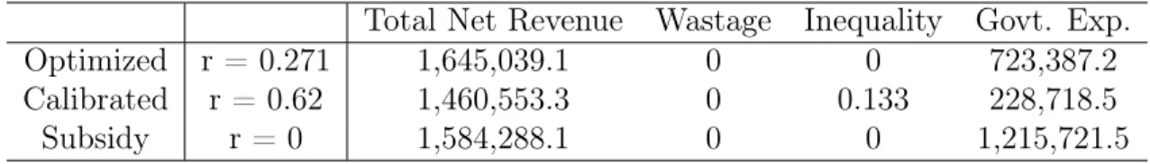
We now consider 3 scenarios: (i) No storage or loans; (ii) Storage but no loan; (iii) Storage and loan. We use the following metrics for comparison: First, total net rev-enue, which we define as harvest season and lean season revenue less cash constraint, across all farmers. Second, wastage, defined as unsold quantity after the lean season. Third, inequality, defined as the proportion of cash constrained farmers. We use this as a metric for inequality because cash constraints are the key driver of sub-optimal decision making in the model, so equality is achieved when no farmers are cash con-strained. This is also justified from a monetary perspective, since all farmers earn equal revenue when no farmers are cash constrained.

We conduct a theoretical analysis to examine the sensitivity of total net revenue, wastage, and inequality to the repayment rate 𝑟. We use 𝑟 because from a government policy perspective, 𝑟 is the means by which the government can control how much money is disbursed to farmers. By setting 𝑟 = 1, the loan model reduces to the base case of no loan, since farmers will opt not to take the loan if they have to repay the full amount. Following the theoretical analysis, we conduct numerical simulations to show how different parameter sets can affect the benefits of storage and loans.

Proposition 5 Define 𝑅1(𝑟) = ∫︀𝐶𝑚𝑎𝑥 0 (𝛼 − 𝛽(𝑞1(𝐶) + (𝑁 − 1)( ^ 𝑐1 𝐶𝑚𝑎𝑥𝐹1+ ˜𝑓1)))𝑞1(𝐶) − 𝐶𝑑𝐶 and 𝑅2(𝑟) = ∫︀𝐶𝑚𝑎𝑥 0 (𝛼 − 𝛽(𝑞2(𝐶) + (𝑁 − 1)( ^ 𝑐2 𝐶𝑚𝑎𝑥𝐹2 + ˜𝑓2)))𝑞2(𝐶) 𝑑𝐶 as harvest

The following equations have unique solutions, denoted as 𝑟1, 𝑟2 and 𝑟3 respectively: ˆ 𝑐1 𝐶𝑚𝑎𝑥 𝐹1+ ˜𝑓1 = 𝛼 2𝛽𝑁 (5.1) (𝛼 − 𝛽(1 − 𝛼 2𝛽𝑁 + (𝑁 − 1)( ˆ 𝑐1 𝐶𝑚𝑎𝑥 𝐹1+ ˜𝑓1))) (1 − 𝛼 2𝛽𝑁) + (1 − 𝑟) 𝛼 2𝛽𝑁𝐿 = 𝐶𝑚𝑎𝑥 (5.2) 1 − ˆ𝑐1 𝐶𝑚𝑎𝑥 𝐹1− ˜𝑓1 = 𝛼 2𝛽𝑁 (5.3)

𝑅1(𝑟) is unimodal, and ∃𝑟*1 ∈ [0, 1] s.t. 𝑅1(𝑟1*) ≥ 𝑅1(𝑟)∀𝑟 ∈ [0, 1], where 𝑟1* is

expressed by the following piece-wise equation:

𝑟₁* = ⎧ ⎪ ⎪ ⎪ ⎪ ⎪ ⎨ ⎪ ⎪ ⎪ ⎪ ⎪ ⎩ 0 𝑟1 ≤ 0 𝑟1 0 < 𝑟1 < 1 1 𝑟1 ≥ 1 For 𝑅2(𝑟), 1. If 𝑟2 ∈ [0, 1] and 𝑟3 ∈ [0, 1], 𝑅/ 2(𝑟2) ≥ 𝑅2(𝑟)∀𝑟 ∈ [0, 1]. 2. If 𝑟2 ∈ [0, 1] and 𝑟/ 3 ∈ [0, 1], 𝑅2(𝑟3) ≥ 𝑅2(𝑟)∀𝑟 ∈ [0, 1]. 3. If 𝑟2, 𝑟3 ∈ [0, 1], 𝑚𝑎𝑥{𝑅/ 2(0), 𝑅2(1)} ≥ 𝑅2(𝑟)∀𝑟 ∈ [0, 1]. 4. If 𝑟2, 𝑟3 ∈ [0, 1], 𝑅2(𝑟2) = 𝑅2(𝑟3) ≥ 𝑅2(𝑟)∀𝑟 ∈ [0, 1]. Define 𝑊 (𝑟) = ∫︀𝐶𝑚𝑎𝑥

0 1 − 𝑞1(𝐶) − 𝑞2(𝐶) 𝑑𝐶 as wastage. The following system of

equations has a unique solution, 𝑟4.

𝐹2 = 1 − 𝐹1 ˆ 𝑐2 = ˆ𝑐1 ˜ 𝑓2 = 1 − ˆ 𝑐1 𝐶𝑚𝑎𝑥 − ˜𝑓1 ˆ 𝑐1 = 𝐶𝑚𝑎𝑥 𝛽(𝑁 − 1){2𝛼 − 2𝛽 − 𝛽(𝑁 − 1) − (1 − 𝑟)𝐿} (5.4)

𝑊 (𝑟) is decreasing in 𝑟 for 𝑟 ∈ [0, 𝑚𝑎𝑥{𝑟4, 0}], and 𝑊 (𝑟) = 0 for 𝑟 ∈ (𝑚𝑖𝑛{𝑟4, 1}, 1].

Define 𝐼(𝑟) = 1 − 𝑐^1

𝐶𝑚𝑎𝑥 and let 𝑞 =

𝛼−(1−𝑟)𝐿

2𝛽𝑁 . The following equation has a unique

solution 𝑟5.

(𝛼 − 𝛽𝑁 𝑞)𝑞 + (1 − 𝑟)(1 − 𝑞)𝐿 = 𝐶𝑚𝑎𝑥 (5.5)

𝐼(𝑟) = 0 for 𝑟 ∈ [0, 𝑚𝑎𝑥{𝑟5, 0}] and increasing for 𝑟 ∈ (𝑚𝑖𝑛{𝑟5, 1}, 1]

From Proposition 5, we see that harvest season revenue is guaranteed to have a unique maximizer, while lean season revenue can have up to 2 maximizers.

The LHS of equation 5.1 is the average quantity sold in the harvest season, while the RHS is the optimal unconstrained quantity _2𝛽𝑁𝛼 . Note that we do not use 𝛼−(1−𝑟)𝐿_2𝛽𝑁 because we want to maximize revenue, not income. When they are equal, harvest season net revenue is maximized. By Proposition 4, we know that a unique solution exists because as 𝑟 decreases, average quantity sold decreases. However, it is possible that the solution is not within the interval [0, 1], in which case the maximizer of 𝑅1(𝑟)

is at the boundary.

Equations 5.2 and 5.3 correspond to the two possible maximizers of 𝑅2(𝑟). Like

the harvest season, lean season revenue is maximized when the average quantity sold is equal to the optimal unconstrained quantity. There are two cases when this may occur: First, when all farmers are able to sell _2𝛽𝑁𝛼 . By Proposition 4, since stored quantity is increasing for all farmers as 𝑟 decreases, there is some unique value where the most cash-constrained farmer stores exactly _2𝛽𝑁𝛼 . This is expressed in equation 5.2, where the LHS is the farmer’s harvest season revenue when selling quantity 1 − _2𝛽𝑁𝛼 . Therefore, the most cash constrained farmer will sell this quantity to meet his cash constraint. Second, in a fully constrained equilibrium, due to differences in quantity stored some farmers are forced to sell less than _2𝛽𝑁𝛼 while others can sell more. As a result, it is possible for the overall average quantity to equal _2𝛽𝑁𝛼 . By Proposition 4, there is a unique value 𝑟3 corresponding to this equilibrium, characterized by

equation 5.3. The LHS is the average quantity stored, while the RHS is the optimal unconstrained quantity. It is not guaranteed that 𝑟2 or 𝑟3 is within the interval [0, 1],

We now move on to the analysis of wastage. From Proposition 4, it is clear that wastage is non-increasing in 𝑟. Since increasing 𝑟 results in decreased stored quantity, wastage cannot increase. In fact, wastage is strictly decreasing in 𝑟 up to the point where the lean season equilibrium transitions from partially constrained to fully constrained, which is characterized by equation 5.4. Recall that we check for the existence of a fully constrained equilibrium by assuming all cash constrained farmers from the harvest season sell all of their stored quantity, then computing the best-response quantity of the remaining unconstrained farmers. The boundary between partially constrained and fully constrained equilibrium is therefore when the best-response quantity of unconstrained farmers is equal to their stored quantity. If 𝑟 is increased, all farmers store less and will therefore sell their maximum quantity, resulting in a fully constrained equilibrium. Hence, wastage is 0 for all greater values of 𝑟. Conversely, if 𝑟 is decreased all farmers store more, and there are fewer cash constrained farmers from the harvest season. As a result, the best-response quantity of the unconstrained farmers decreases, and we have a partially constrained equilibrium. Hence, wastage increases.

Finally, with regard to inequality, from Proposition 4 we know that inequality is non-decreasing in 𝑟. In fact, inequality is constant at 0 to the point where the har-vest season equilibrium transitions from unconstrained to partially constrained, after which inequality is strictly increasing. To find the boundary between unconstrained and partially constrained equilibria, we use the result from Theorem 3 to find the value of 𝑟 such that the most cash constrained farmer just meets his cash constraint by selling the optimal unconstrained quantity. This condition is expressed in equation 5.5.

For the numerical simulations, Figures 5-1 and 5-2 illustrate how total net rev-enue, wastage, and inequality change in response to changes in 𝛼 and 𝐶𝑚𝑎𝑥, under 3

scenarios: (i) no storage or loan, (ii) storage but no loan, (iii) storage and loan. We exclude 𝛽 and 𝑁 since the results are similar. Note that scenarios (i) and (ii) are unaffected by 𝑟, so the lines are constant. Also note that providing storage does not affect inequality, so we only show scenarios (i) and (iii) in the inequality plot.

Figure 5-1: Simulation results for the following parameter values: 𝛽 = 0.1, 𝑁 = 520, 𝐶𝑚𝑎𝑥 = 16, 𝐿 = 10.

Figure 5-2: Simulation results for the following parameter values: 𝛼 = 30, 𝛽 = 0.01, 𝑁 = 1800, 𝐿 = 10.

We begin by analyzing Figure 5-1. For this parameter set, note that optimal unconstrained quantity _2𝛽𝑁𝛼 = 0.48 when 𝛼 = 50. This indicates that if farmers were not cash constrained, it would be optimal for them to waste a significant amount of produce in the harvest season. Therefore, if storage were provided, we expect a large quantity to be stored, and farmers would see a large increase in revenue. This is reflected in the total net revenue plot for 𝛼 = 50, where farmers saw a 393% increase in net revenue from storage. In comparison, loans provide a relatively small improvement in net revenue. The wastage plot highlights one of the drawbacks of loan provision, as it becomes optimal for farmers to waste produce as 𝑟 decreases. Decreasing 𝑟 also serves to reduce inequality, establishing the trade-off between reducing wastage and inequality. However, for 𝛼 = 55, there is a range of 𝑟 values where we have zero wastage and inequality simultaneously. In increasing 𝛼 = 50 to 𝛼 = 55, we improve market price conditions and increase the optimal unconstrained quantity. Storage is therefore utilized less, but still provides a 184% increase in revenue. Loans provide even smaller benefit than before, because taking a loan is now a less attractive option for farmers compared to selling their produce on the market. With better prices, more farmers can meet their cash constraint and there is less reason to take a loan. The reduction in cash constrained farmers is clear in the inequality plot. Finally, wastage is reduced because better prices incentivize farmers to sell more of their produce on the market.

For Figure 5-2, the optimal unconstrained quantity is now 0.83. As a result, it is optimal for farmers to sell almost all of their produce in the harvest season. Therefore, storage has less of an impact on net revenue, which only increases 68%. This parameter set demonstrates how loans can be used to encourage usage of storage and thereby boost revenue. For 𝐶𝑚𝑎𝑥 = 13 and 𝑟 = 0, the loan improves revenue by a

further 43%, relative to the storage and no loan case. Because of the higher optimal unconstrained quantity, it is optimal for farmers to sell all of their produce over the harvest and lean seasons. This is reflected in the wastage plots, where we have zero wastage for scenarios (ii) and (iii). Note that the effect on net revenue and inequality when reducing 𝐶𝑚𝑎𝑥 from 14 to 13 is very similar to that of increasing 𝛼 from 50 to

55. This reflects the point in Chapter 3 that both of these parameter shifts have the effect of making it easier for farmers to meet their cash constraints. Therefore, we intuitively expect these changes to have similar results.

Chapter 6

Government Optimization Problem

We consider the scenario where the government has provided storage and determined 𝐿, and now wants to find the optimal 𝑟 that maximizes government utility. We propose the following objective function:

𝑚𝑎𝑥𝑟 𝑤1{ ∫︁ 𝐶𝑚𝑎𝑥 0 (𝛼 − 𝛽(𝑞1(𝐶) + (𝑁 − 1)( ˆ 𝑐1 𝐶𝑚𝑎𝑥 𝐹1+ ˜𝑓1)))𝑞1(𝐶) − 𝐶 𝑑𝐶 + ∫︁ 𝐶𝑚𝑎𝑥 0 (𝛼 − 𝛽(𝑞2(𝐶) + (𝑁 − 1)( ˆ 𝑐2 𝐶𝑚𝑎𝑥 𝐹2+ ˜𝑓2)))𝑞2(𝐶) 𝑑𝐶} −𝑤2{ ∫︁ 𝐶𝑚𝑎𝑥 0 1 − 𝑞1(𝐶) − 𝑞2(𝐶) 𝑑𝐶} −𝑤3{1 − ˆ 𝑐1 𝐶𝑚𝑎𝑥 }

The objective function is the weighted sum of total farmer net revenue, wastage, and inequality, as defined in Chapter 5. To characterize the objective function maximizer 𝑟*, we begin by considering the edge case where 𝑤2 = 𝑤3 = 0. Following that, we

examine how the inclusion of wastage and inequality affects 𝑟*. Finally, we conclude by summarizing the implications on government policy.

Recall from Proposition 5 that harvest season net revenue has a unique maximizer, while lean season net revenue has up to two maximizers. For the following analysis, we assume that all three maximizers are in the interval [0, 1]. Denote the maximizers 𝑟1, 𝑟2 and 𝑟3, as defined in Proposition 5. Let the total net revenue maximizer be 𝑟*𝑟𝑒𝑣.

Proposition 6 1. If _2𝛽𝑁𝛼 ≥ 1, 𝑟* 𝑟𝑒𝑣 ∈ (0, 2𝛽𝑁 −(𝛼−𝐿) 𝐿 ) 2. If 1₂ < _2𝛽𝑁𝛼 < 1, 𝑟2 ≤ 𝑟3 < 𝑟𝑟𝑒𝑣* < 𝑟1 3. If _2𝛽𝑁𝛼 = 1 2, 𝑟2 ≤ 𝑟3 = 𝑟1 = 𝑟 * 𝑟𝑒𝑣 4. If 0 < _2𝛽𝑁𝛼 < 1₂, then for 𝑟 = 𝑟1, (a) If 1 − 𝑞1(𝐶𝑚𝑎𝑥) > _2𝛽𝑁𝛼 , 𝑟1 < 𝑟𝑟𝑒𝑣* < 𝑟2 < 𝑟3 (b) If 1 − 𝑞1(𝐶𝑚𝑎𝑥) = _2𝛽𝛼, 𝑟𝑟𝑒𝑣* = 𝑟1 = 𝑟2 < 𝑟3 (c) Else, 𝑟2 < 𝑟𝑟𝑒𝑣* < 𝑟3

If _2𝛽𝑁𝛼 ≥ 1, it is optimal for farmers to sell 1 unit in the harvest season until 𝑟 decreases to the point that 𝛼−(1−𝑟)𝐿_2𝛽𝑁 < 1. Since farmers will earn maximum revenue by selling 1 unit, harvest season net revenue is maximized for all 𝑟 ≥ 2𝛽𝑁 −(𝛼−𝐿)_𝐿 . For the lean season, it is always optimal for farmers to sell all of their stored quantity. Lean season revenue is thus maximized for 𝑟 = 0, where quantity stored is maximized. 𝑟*_𝑟𝑒𝑣 is thus in the interval (0,2𝛽𝑁 −(𝛼−𝐿)_𝐿 ).

If 1₂ < _2𝛽𝑁𝛼 < 1, since farmers only have 1 unit to sell over the harvest and lean season, if harvest season net revenue is maximized, farmers will store insufficient quantity to maximize lean season revenue. Hence we have 𝑟2 ≤ 𝑟3 < 𝑟1, and since

harvest season net revenue is unimodal by Proposition 5, 𝑟*_𝑟𝑒𝑣 is in the interval (𝑟3, 𝑟1).

If _2𝛽𝑁𝛼 = 1

2, farmers will maximize harvest season and lean season net revenue at

the same time, hence we have 𝑟2 ≤ 𝑟3 = 𝑟1 = 𝑟𝑟𝑒𝑣* .

If 0 < _2𝛽𝑁𝛼 < 1₂, when farmers maximize harvest season net revenue, they will store too much to maximize lean season revenue with a fully constrained equilibrium. Hence we have 𝑟1 < 𝑟3. However, the relationship between 𝑟1 and 𝑟2 is dependent

on the quantity stored by the farmer with cash constraint 𝐶𝑚𝑎𝑥, 1 − 𝑞1(𝐶𝑚𝑎𝑥). If,

at 𝑟 = 𝑟1, 1 − 𝑞1(𝐶𝑚𝑎𝑥) > _2𝛽𝑁𝛼 , then the farmer is storing more than enough to sell

the optimal unconstrained quantity. Hence 𝑟1 < 𝑟2 < 𝑟3, and 𝑟*𝑟𝑒𝑣 is in the interval

(𝑟1, 𝑟2). If 1 − 𝑞1(𝐶𝑚𝑎𝑥) = _2𝛽𝑁𝛼 , we have 𝑟1 = 𝑟2 < 𝑟3, and 𝑟*𝑟𝑒𝑣 = 𝑟1. Finally, if

From Proposition 5, wastage is non-increasing in 𝑟. Therefore, as 𝑤2 increases,

we expect 𝑟* to increase. However, note that if 𝑟*_𝑟𝑒𝑣 ≥ 𝑟4, where 𝑟4 is the solution to

equation 5.4, then 𝑟* = 𝑟_𝑟𝑒𝑣* since there is zero wastage at 𝑟*_𝑟𝑒𝑣. Conversely, inequality is non-decreasing in 𝑟, and we expect 𝑟* to decrease as 𝑤3 increases. However, if

𝑟*_𝑟𝑒𝑣 ≤ 𝑟5, where 𝑟5 is the solution to equation 5.5, then 𝑟* = 𝑟𝑟𝑒𝑣* since there is zero

inequality at 𝑟*_𝑟𝑒𝑣. Note that due to the multimodal nature of net revenue, we cannot guarantee the existence of a unique 𝑟*.

As a robustness check, we also consider adding an additional term to the objective function for government expenditure, computed as the proportion of the loan that is not paid back by farmers.

∫︁ 𝐶𝑚𝑎𝑥

0

(1 − 𝑟)(1 − 𝑞1(𝐶))𝐿 𝑑𝐶

Similar to wastage, we find that government expenditure is decreasing in 𝑟, and becomes constant at 0 when it is optimal for farmers to sell everything in the harvest season. We find that the inclusion of government expenditure in the objective function does not affect our prior findings on 𝑟*.

We now examine policy insights that can be drawn from the analysis. Since the provision of storage infrastructure gives farmers a mechanism to transfer quantity across periods, it is clear that all farmers with excess quantity in the harvest season will obtain greater revenue, as well as reduced wastage. Whether the investment in storage facilities will be worthwhile is strongly dependent on the nature of the harvest season market. If demand outpaces supply, storage facilities may be underutilized. However, the government must be cognizant that farmers may be forced to sell larger quantities than they would prefer in the harvest season due to their cash constraints. In this case, offering a loan can be an effective mechanism to increase the benefits from storage. The crux of the optimization problem then lies in the loan quantum and repayment rate, which allows the government to control how much quantity farmers store.

Figure 6-1: Lean season total revenue.

and wastage. On one hand, improving equality requires decreasing 𝑟 so that cash constrained farmers can afford to store more. However, generous loan terms can create a wastage problem as it disincentivizes unconstrained farmers from selling their produce on the market during the harvest season. They would rather store excess quantity to take a larger loan, even if much of that stored quantity goes unsold in the lean season. On the other hand, by increasing 𝑟, it is possible to achieve zero wastage. We plot lean season total revenue as a function of 𝑟 in Figure 6-1. We have zero wastage at 𝑟3 where we have a fully constrained equilibrium, and we achieve the

same total revenue as at 𝑟2, where we have an unconstrained equilibrium and total

lean season revenue is maximized. However, total revenue as a metric fails to reflect the distribution of revenue amongst farmers. At 𝑟3, cash-constrained farmers are in

fact doubly worse off relative to their peers - not only do they have less net revenue in the harvest season, they also have less quantity and therefore less revenue in the lean season.

Another crucial insight is that decreasing 𝑟 does not necessarily improve total revenue in the first or lean season. In the harvest season, this occurs when average quantity sold declines below _2𝛽𝑁𝛼 . Since the loan offering can be interpreted as an

alternative ’market’ where the farmer can sell his produce for a price of (1 − 𝑟)𝐿, the government should be cautious of offering terms that overly disincentivize farmers from selling their produce on the actual market.

In the lean season, total revenue can decline if the average quantity sold exceeds

𝛼

2𝛽𝑁. This is seen in Figure 6-1 where total revenue initially decreases as 𝑟 is decreased

past 𝑟3. This is a result of the uneven distribution of quantity amongst farmers.

Farmers with greater quantity know that their peers are quantity constrained and therefore flood the market, driving prices down. As 𝑟 is decreased further, total revenue gradually reverts to the optimal level as stored quantity becomes increasingly uniform across farmers. Total revenue in the lean season can also remain constant if all farmers are able to sell _2𝛽𝑁𝛼 . On Figure 6-1, this is represented by 𝑟 < 𝑟2. Further

reducing the repayment rate will increase the quantity stored but not the quantity sold, resulting in increased wastage.

Therefore, on top of balancing the need to improve farmer revenue and equality amongst farmers with the desire to limit wastage, the government must also be aware that offering improved loan terms can backfire by reducing farmer revenue.

Chapter 7

Relating Model Predictions to

Empirical Observations

In this chapter, we calibrate our model parameters with field data to examine the extent to which storage and loan provision can improve farmer outcomes, as measured by total net revenue, wastage, and equality. We consider 4 scenarios: (i) the base case without storage or loans; (ii) intervention using calibrated values of 𝐿 and 𝑟; (iii) intervention using the calibrated value of 𝐿 and the optimized value of 𝑟; (iv) intervention using the calibrated value of 𝐿 and 𝑟 = 0. The last case effectively means the government provides a subsidy for farmers, and we include it because of the numerous instances of Indian state governments offering loan waivers to farmers [19]. Given the popularity of such schemes, we feel that it is worth analyzing.

We use field data from Bengal gram farmers in Karnataka state. We use Karnataka because agriculture is the dominant industry for the rural population, supporting over 60% of the workforce and occupying over 64% of state land [2]. Furthermore, 79% of farmer households are smallholders occupying less than 2 hectares of land [22]. Karnataka is also India’s fourth largest producer of Bengal gram, which is cultivated in 70% of the land in North Karnataka during the dry season [27]. Despite the Bengal gram’s popularity, many Bengal gram farmers suffer from poverty. In early 2020, farmers launched a state-wide protest demanding increased government assistance for farmers. A key complaint was that due to a lack of storage facilities for grams,

𝛼 𝛽 𝑁 𝐶𝑚𝑎𝑥 𝐿 𝑟

85960.91 215.89 248 44580.87 44500 0.62 Table 7.1: Calibrated parameter values.

farmers were forced to accept low prices offered by traders, negatively influencing farmer revenue [1]. Therefore, there is certainly a pressing need to help farmers, and we believe that storage and loan provision are feasible interventions to be considered. We calibrate the price parameters 𝛼 and 𝛽, as well as the number of farmers 𝑁 using data from the Unified Market Platform as well as demographic data from the Karnataka state government. We estimate 𝐶𝑚𝑎𝑥 using cost of production and

income data from the Ministry of Agriculture and Farmers Welfare [23][6]. Finally, we estimate 𝐿 and 𝑟 using information from the National Bank for Agriculture and Rural Development [18] and state data [5].

Table 7.1 summarizes the parameter values used in our analysis. 𝛼 and 𝛽 are ob-tained by linear regression, using weekly price and quantity data for markets across Karnataka. 𝑁 is obtained by averaging the number of farmers that sold produce during the harvest season over the number of markets. 𝐶𝑚𝑎𝑥 is obtained from cost

of production data from the Commission for Agricultural Costs and prices, less the average farming households’ monthly income from non-agricultural sources. We es-timate 𝐿 to be slightly lower than 𝐶𝑚𝑎𝑥, using the state government’s guidelines for

determining the loan quantum that farmers are eligible for, and 𝑟 is obtained from data on loan repayment rates.

We find that without storage and loans, some farmers are unable to meet their cash constraint, and consequently there is no feasible solution. We find that the maximum value of 𝐶𝑚𝑎𝑥 for a feasible equilibrium to exist is 39450. Consequently,

assuming farmers have uniformly distributed cash constraints, at least 11.5% of farm-ers are unable to meet their cash constraints without government assistance. This is consistent with reports of farmers struggling to recoup their cost of production.

Using the calibrated value 𝑟 = 0.62, all farmers can meet their cash constraints. The equilibrium value of ˆ𝑐1 is 38636, indicating that 13.3% of farmers are cash