Dynamic response of graphite/epoxy plates subjected to impact loading

by

Kiernan Francis Ryan B.S.E., Arizona State University

(1987)

Submitted to the Department of Aeronautics and Astronautics in partial fulfillment of

the requirements for the degree of Master of Science

in Aeronautics and Astronautics at the

Massachusetts Institute of Technology February 1990

@ Massachusetts Institute of Technology 1989

Signature of Author

Department of Aeronautics and Astronautics September 18, 1989 Certified by Accepted by kMASSACHUSETTS INSTITUTE OF Tr '' . •""y

FEB 2

6

1990

Professor Paul A. Lagace Thesis Supervisor

z7.-" .:z7.-":Pro0fessOr Eko1d Y. Wachman Chairman, Departmental Graduate Committee

Aero

DYNAMIC RESPONSE OF GRAPHITE/EPOXY PLATES

SUBJECTED TO IMPACT LOADING

by

Kiernan Francis Ryan

Submitted to the Department of Aeronautics and Astronautics on September 18, 1989 in partial fulfillment of the requirements for the Degree of Master of

Science

ABSTRACT

The dynamic response of graphite/epoxy plates subjected to impact load-ing was investigated experimentally and analytically. The material system used was Hercules AS4/3501-6 prepreg tape. Plates of [0/90]5s and [±45/0]1s

layups with a test area of 89 mm by 344 mm were tested. The dynamic response was investigated on a local level and a global level. The local level was investigated experimentally with quasi-static tests and the global level was investigated with instrumented impact tests. These tests were carried out on virgin and predamaged specimens. The damage in the predamaged speci-mens was introduced by impacting laminates with a 1.53 kg impactor rod with a 6.35 mm radius hemispherical tup at a velocity of 4.0 m/s. The amount of damage was determined from visual and dye-penetrant-enhanced X-ray tech-niques to consist of small matrix cracks on the back surface and internal damage the size of the impactor diameter. The presence of damage was found to increase the contact stiffness at the local level due to the surface of a dam-aged laminate being more able to conform to the shape of the indentor. This dependence on the area of contact means that the contact relation will depend on the curvature of the surface. The presence of damage was found not to affect the global structural response recorded as force and displacement histo-ries of the center of the plate. This means that the global analysis does not need to account for the presence of local damage in laminates. The analytical study at the local level produced load versus indentation data that agrees well with the experimental results. The experimental load versus indentation data was fit to a general form of the Hertzian contact law. This relation proved to be inadequate to accurately model the experimental results. The analytical force and displacement histories do not agree well with the experimental results. However, they do capture the general shape of the histories as well as the phe-nomenon of the impactor losing contact with the plate and then recontacting it early in the impact event. More work needs to be done to bring the global anal-ysis into better agreement with the experimental data.

Thesis Supervisor: Paul A. Lagace

Title: Associate Professor, Department of Aeronautics and Astronautics, Massachusetts Institute of Technology

As Prof. Paul Lagace has said, it is not the expensive equipment that makes up TELAC, but the people. I am thankful that I was able to work in this laboratory because of the many friendly people here. A special thanks to Paul for making it be this way - you do an outstanding job.

I would like to thank the UROPers. Chris Park did an excellent job on the computer programs and the operation of the ACPI system. Randy Notestine and Claudia Ranniger provided much help and suggestions during the experimental phase of the research. They did an outstanding job in the laboratory for me (except for the cleaning of my laminates with acetone) and required little supervision (which was useful when I was studying for the qualifying exam). I wish them luck on their masters work. Suzanne Starnes provided much help in the data reduction of the experimental data as well as assist in some of the experiments. Thanks for your help.

Thanks to all of the graduate students for their help and friendships. Thanks to Simon Lie, Wilson Tsang, Kevin Saeger, and Pierre Minguet for tak-ing the time to answer my many questions. A special thanks to Pierre who provided the ground work for the new time marching routine used in the global analysis.

Finally, I would like to thank the TELAC staff and professors. Thanks to Al Supple for much help in the laboratory and opening my eyes to the real world of machine shop work. Thanks to Prof. Michael Graves who partici-pated in many of my meetings with Paul. Thanks to Prof. John Dugundji who always had an open door to answer some of my questions.

Foreword

This work was conducted at TELAC (Technology Laboratory for Advanced Composites) of the Department of Aeronautics and Astronautics at the Massachusetts Institute of Technology.

Table of Contents

PTFAG

2.3 Impactor/Plate Contact Relation 27

3 ANALYTICAL METHODS 31

3.1 Analysis Overview 31

3.2 Local Model 32

3.3 Global Model 36

3.3.1 Overview 36

3.3.2 Improved Time-Marching Scheme 40

3.4 Computer Implementation 55

3.5 Numerical Example 57

4 EXPERIMENTAL PROCEDURES 79

4.1 Test Matrix and Specimen Description 79

4.2 Manufacturing Procedures 85

4.3 Test Procedures 90

4.3.1 Static Indentation Tests 90

4.3.2 Impact Tests 96

CHAPTER

PAGI

5 EXPERIMENTAL RESULTS 112

5.1 Impactor/Plate Contact Relation 112

5.1.1 Undamaged Laminates 114

5.1.2 Damaged Laminates 126

5.2 Dynamic Impact Response 132

5.2.1 Undamaged Laminates 132

5.2.2 Damaged Laminates 144

6 ANALYTICAL COMPARISON AND DISCUSSION 159 6.1 Impactor/Plate Contact Relation 159

6.2 Dynamic Impact Response 174

7 CONCLUSIONS AND RECOMMENDATIONS 191

REFERENCES 195

APPENDIX A: FORTRAN Source Codes 197

APPENDIX B: Operation of ACPI (Analysis of Composite Plate 367 Impact)

List of Figures

GURE

3.1 Local contact problem schematic. 3.2 Rigid indentor contact schematic.

3.3 Schematic of laminated plate impact model.

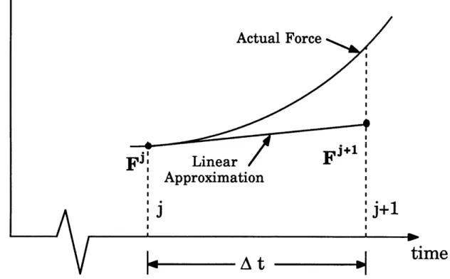
3.4 Illustration of linearization of the forcing function at the

jth time step.

3.5 Impact analysis flow chart.

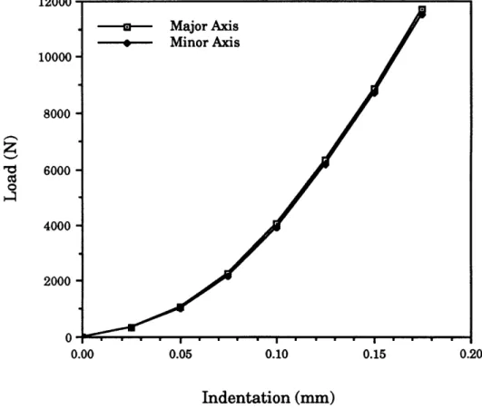
3.6 _{Analytical impactor/plate contact relation for a [±}4 5_/012s layup of AS4/3501-6.

3.7 Comparison of the assumed pressure distribution with the recovered pressure distribution. (Half of the

axisymmetric distributions are shown.)

3.8 Convergence of the recovered load for the major axis analysis with an approach of 0.05 mm.

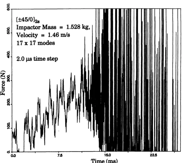
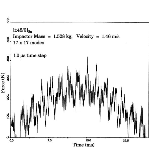
3.9 Analytical force history of a [±45/0]2s laminate using 9 x 9 modes. 3.10 Analytical force 13 x 13 modes. 3.11 Analytical force 17 x 17 modes. 3.12 Analytical force 2.0 gs time step. 3.13 Analytical force 1.0 ps time step. 3.14 Analytical force 0.5 ps time step.

history of a [±4 5_/0]2s 1 _{laminate using}

history of a [I45/0]2s laminate using

history of a [±4 5_{/0]2s laminate using a}

history of a [±4 5_{/0]2s laminate using a}

history of a [±4 5_/01_{]2s laminate using a}

PAGE

List of Figures (continued)

FIGURE

3.15 Analytical displacement history of a [±45/012s laminate using 9 x 9 modes.

3.16 Analytical displacement history of a [±45/0]2s laminate using 13 x 13 modes.

3.17 Analytical displacement history of a [±45/012s laminate using 15 x 15 modes.

4.1 Test specimen geometry.

4.2 Geometry of 6-32 machined nut. 4.3 Cure assembly cross section.

4.4 Curing schedule for AS4/3501-6 graphite/epoxy. 4.5 Location of specimen width and thickness

measurements.

4.6 Illustration of bonding setup for machined nut. 4.7 Illustration of test setup for static indentation test. 4.8 Illustration of specimen holder for static indentation

tests of [0/9015s specimens.

4.9 llustration of the location of the clamping rods for the static indentation tests of [±45/012s specimens.

4.10 Illustration of specimen holding jig for impact tests. 4.11 Illustration of impactor unit.

4.12 Illustration of striker unit.

4.13 Illustration of experimental displacement measurement. 4.14 Free-body diagrams of the impactor rod.

PAGE

83

84

86

88

89

91

93

97

98

List of Figures (continued)

FIGURE

4.15 Plot of force versus time for the impactor rod hit by the striker unit.

4.16 Results of Fast Fourier Transform to obtain

experimental frequencies of the impactor rod when struck by the striker unit.

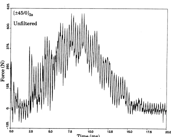
4.17 Typical impact force history of a [±4 5_{/012s undamaged}

laminate with the stress wave present.

4.18 Fast Fourier Transform of the force history of the [±45/012s undamaged laminate (of Figure 4.17). 4.19 Impact force history of the [±45/012s undamaged

laminate with the stress wave suppressed. 5.1 Typical plot of force versus indentation data.

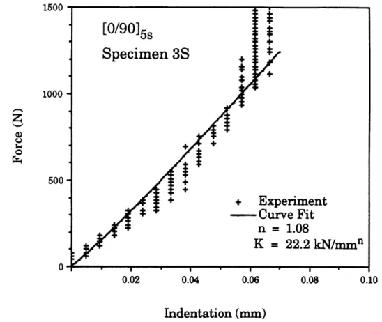
5.2 Typical plot of log of force versus log of indentation data. 5.3 Plot of load versus indentation for [0/9 015s specimen 1S. 5.4 Plot of load versus indentation for [0/9 015s specimen 2S. 5.5 Plot of load versus indentation for [0/9 0 1_{5s specimen 3S.}

5.6 _{Plot of load versus indentation and curve fit for [0/9015s} specimen 3S.

5.7 Plot of load versus indentation for [±4 5/012s undamaged specimen 1SU.

5.8 Plot of load versus indentation for [±4 5/0]2s undamaged specimen 2SU.

5.9 Plot of load versus indentation for [±4 5/012s undamaged specimen 3SU.

PAGE

List of Figures (continued)

PAGE

5.10 X-ray of a [±45/012s specimen impacted with a 1.53 kg impactor at 4.0 m/s.

5.11 Plot of load versus indentation for [±4 5_{/0]2s damaged}

specimen 1SD.

5.12 Plot of load versus indentation for [±45/012s damaged specimen 2SD.

5.13 Plot of load versus indentation for [±45/01]2 damaged

specimen 3SD.

5.14 Filtered force history of [0/9 015s specimen 1.5 m/s.

5.15 Filtered force history of [0/9 015s specimen 1.4 m/s.

5.16 Filtered force history of [0/9 015s specimen 1.5 m/s.

5.17 Filtered force history of [0/9015s specimen extension rod impacted at 1.6 m/s.

11 impacted at

21 impacted at

31 impacted at

without the

5.18 Center displacement history of [0/9 0_{15s specimen 11I}

impacted at 1.5 m/s.

5.19 Center displacement history of [0/9 0_{15s specimen 21}

impacted at 1.4 m/s.

5.20 Center displacement history of [0/9 0_{15s specimen 31}

impacted at 1.5 m/s.

5.21 Filtered force history of [±45/012s undamaged specimen 1IU impacted at 1.5 m/s. 127 128 129 130 133 134 135 137 138 139 140 141

List of Figures (continued)

5.22 _{Filtered force history of [±45/012s}

2IU impacted at 1.4 m/s.

5.23 _{Filtered force history of [±45/012s} 3IU impacted at 1.5 m/s.

undamaged specimen

undamaged specimen

5.24 Filtered force history of [±45/012s undamaged specimen without the extension rod impacted at 1.5 m/s.

5.25 Center displacement history of [±45/012s undamaged specimen IHU impacted at 1.5 m/s.

5.26 Center displacement history of [±45/012s undamaged specimen 2IU impacted at 1.4 m/s.

5.27 Center displacement history of [±45/012s undamaged specimen 3IU impacted at 1.5 m/s.

5.28 _{Filtered force history of [±45/012s} at 3.9 m/s.

5.29 _{Filtered force history of [±45/012s} at 4.0 m/s.

5.30 _{Filtered force history of [±45/012s} at 4.0 m/s.

5.31 _{Filtered force history of [±45/012s} 4ID impacted at 1.4 m/s.

5.32 _{Filtered force history of [±45/012s} 5ID impacted at 1.5 m/s.

5.33 _{Filtered force history of [±45/012s} 6ID impacted at 1.5 m/s.

specimen 4ID impacted

specimen 5ID impacted

specimen 6ID impacted

predamaged specimen predamaged specimen predamaged specimen 142 143 145 146 147 148 149 150 151 153 154 155

List of Figures (continued)

GURE

PAG1

5.34 Center displacement history of [±45/0]2s predamaged 156 specimen 4ID impacted at 1.4 m/s.

5.35 Center displacement history of [±45/012s predamaged 157 specimen 5ID impacted at 1.5 m/s.

5.36 Center displacement history of [±45/012s predamaged 158 specimen 6ID impacted at 1.5 m/s.

6.1 Convergence of the load versus indentation curves 161 obtained from the analysis of a [0/9015s laminate.

6.2 Analytical results and experimental data for static 162 indentation of [0/9015r laminates.

6.3 Analytical results and experimental data for static 165 indentation of [±45/012s laminates.

6.4 Illustration of (a) Analytical assumption of the 168 deformation of the plate due to a contact load; and

(b) Physical deformation of the plate due to a contact load. 6.5 Illustration of Hertzian loading distribution. 169 6.6 The experimental impactor/plate contact relations for a 170

[±45/012s laminate and a [0/9015s laminate.

6.7 The analytical impactor/plate contact relations for a 172 [±45/012s laminate and a [0/9015s laminate.

6.8 Experimental impactor/plate contact relations for a 173 damaged and undamaged [±45/012s laminate.

6.9 Analytical force history of a [0/9015s laminate impacted at 177 1.52 m/s with a 1.53 kg impactor.

6.10 Fast Fourier Transform of the filtered experimental 178 force data for a [0/9015s laminate - specimen 31.

List of Figures (continued)

FIGUREPAG

6.11 Fast Fourier Transform of the analytical force data for a 179 [0/9015s laminate.

6.12 Analytical and experimental (specimen 31) 181 displacement histories of a [0/90]5s laminate impacted at

1.52 m/s with a 1.53 kg impactor.

6.13 Analytical force history of a [±45/012s laminate impacted 183 at 1.46 m/s with a 1.53 kg impactor.

6.14 Fast Fourier Transform of the filtered experimental 185 force data for a [±4 5/012s laminate -test of specimen

without the extension rod.

6.15 Fast Fourier Transform of the analytical force data for a 186

[±45/012s laminate.

6.16 Analytical and experimental (test of specimen without 187 the extension rod) displacement histories of a [±4 5_/01]2s

laminate impacted at 1.5 m/s with a 1.53 kg impactor.

APPENDIX FIGURE

List of Tables

TABLAE PAGE

3.1 AS4/3501-6 Graphite/Epoxy Ply Properties 59 3.2 [i4 5/0]2s AS4/3501-6 Equivalent Engineering Properties 60 3.3 Major Axis and Minor Axis Material Property Inputs 61 3.4 Reduced Data From the Local Model Analysis 66 3.5 [±45/012s AS4/3501-6 Plate Bending and Shear Properties 68

4.1 Quasi-Static Test Matrix 80

4.2 Impact Test Matrix 82

4.3 Impactor Rod Natural Frequencies 107

5.1 Reduced Data From Experimental Static Indentation 119 Tests of [0/9 0 15s Specimens

5.2 Reduced Data From Experimental Static Indentation 125 Tests of [±4 5/012s Undamaged Specimens

5.3 Reduced Data From Experimental Static Indentation 131 Tests of [±4 5_/01_{2s Damaged Specimens}

6.1 Inputs for Local Analysis of [0/90]5s AS4/3501-6 160 Laminates

6.2 Inputs for Local Analysis of [±45/012s AS4/3501-6 164

Laminates

6.3 Inputs for Global Analysis of [0/9015s AS4/3501-6 175 Laminates

6.4 Inputs for Global Analysis of [±45/012s AS4/3501-6 182 Laminates

Nomenclature

a acceleration of the impactor; length of the plate in x-direction ai constants in Eqs. (3.18) and (3.19)

A constant of integration; constant in the beam functions b length of the plate in y-direction

bi constants in Eq. (3.19)

Am constants in Eq. (3.3)

B constant of integration; constant in the beam functions Bm constants in Eq. (3.3)

ci constants in Eq. (3.27)

(C) vector of time-varying displacement modal amplitudes {i) vector of time-varying acceleration modal amplitudes Cm constants in Eq. (3.3)

CW scalar defined by Eq. (3.59) di constants in Eq. (3.27)

Dm constants in Eq. (3.3)

fm function defined by Eq. (3.3) FFT force at the force transducer

FTot force at tip of tup

gm function defined by Eq. (3.1)

Nomenclature (continued)

[K] stiffness matrix defined by Eq. (3.11)

[K*] statically condensed stiffness matrix of plate

m mass of the impactor; number of modes in the x-direction for the global analysis

mk beam function in x-direction [M] mass matrix of plate

MFT mass of the force transducer

MRod mass of the impactor rod MTup mass of the the tup

n number of modes in the y-direction for the global analysis; exponent in the contact relation of Eq. (2.1)

nk beam function in y-direction

r radial coordinate

R contact force

{Re) forcing function vector

Rd radius of plate analyzed in the local model

s1 constant found from the material properties of the plate s2 constant found from the material properties of the plate

t time

tj time at the

jth

u displacement of the top surface of the plate under the indentor; displacement of the impactor

Nomenclature (continued)

velocity of the impactor acceleration of the impactor

displacement of the bottom surface of the plate under the indentor; displacement of the midplane of the plate under the impactor in the global analysis

velocity of plate under the impactor

product of the kth beam function in the x-direction and the kth beam function in the y-direction

modal amplitude defined by Eq. (3.12) first time derivative of (Y)

second time derivative of {Y} local indentation of plate scalar defined by Eq. (3.24) constants in the beam functions size of time step

a small positive number

constant in the beam functions

roots of the Bessel function of the first kind dimensionless coordinate of plate in x-direction dimensionless coordinate of plate in y-direction

v

Wk

Nomenclature (continued)

{t} eigenvector satisfying Eq. (3.17)

c eigenvalue satisfying Eq. (3.17)

CHAPTER 1

Introduction

The aircraft industry has been increasing its use of advanced composite materials for secondary and primary load-bearing members. The General Dynamics F-111 has a composite horizontal tail and fuselage section. The McDonnell Douglas F-15 has composite vertical and horizontal stabilizers. Recently two airframes have been designed and constructed entirely with advanced composite materials. They are the Beechcraft Starship I aircraft

and the Boeing Model 360 helicopter.

One major concern in the design of composite structures is their response to impact. Their response differs from metals because of the orthotropic and laminated nature of composite materials. For example, a composite part may be impacted and show no visible damage, yet have internal damage which significantly reduces the load-carrying capacity of the part. A metal part, on the other hand, will typically have externally visible damage.

Since aircraft structures are subjected to impacts such as tool drop, runway kickup, and bird strikes, it is important for engineers to have an understand-ing of the response of composite materials to such events. Engineers design-ing and analyzdesign-ing these structures need analyses which would aid them in

designing parts to meet any specified requirements related to impact.

A number of investigators have previously done work on developing such analyses. These analyses start by predicting the dynamic response of the composite structure to an impact event. The results of the dynamic response

analysis coupled with other appropriate analyses may be used to predict dam-age in the structure and, ultimately, the residual strength.

The response of the structure to an impact is assumed to occur at two levels - a global response of the structure and a local response under the point of impact. The analysis and experiments are thus broken down into these two segments. The global response is experimentally investigated by dynamic tests. Force and displacement time histories are experimentally measured during these tests. The local response is investigated by quasi-static tests.

The present research effort centers on experimentally investigating the dynamic response of an impacted composite plate. Specifically, the effect of damage on the dynamic response is investigated. One of the reasons for inves-tigating this is because existing analyses generally assume that damage does not affect the local or global response during the event. The validity of this assumption has not been previously investigated. The experiments in the pre-sent research effort are designed such that the specimen remains undam-aged. These experiments are conducted with virgin specimens and specimens which have been damaged from a previous impact (an impact with enough energy such that damage results). The results from these tests are compared to determine the effects of damage. This should provide insight to the physics of the impact event, as well as allow a check on the validity of the no damage assumption in existing analyses.

In Chapter 2, previous work done in the area of impact to composite plates is discussed. In Chapter 3, the analytical methods are described, and the differences between the present analyses and a previous analysis is high-lighted. In Chapter 4, the methods used to manufacture the test specimens

and conduct the experiments are described. In Chapter 5, the experimental results are presented. In Chapter 6, the analytical results are presented and

discussed in light of the experimental results. In Chapter 7, the conclusions and recommendations are given. Finally, the FORTRAN source code is con-tained in Appendix A and an outline on how to use the codes in Appendix B.

CHAPTER 2

Previous Work

2.1 Overview

The impact of a foreign object to a composite plate is a complex event occurring over a very short period of time (on the order of milliseconds). For this reason, it is convenient to break the event down and analyze one part at a time. The impact event may be separated into the three following areas [1]: the dynamic behavior of the composite plate during impact, the local damage induced from the impact (damage resistance), and the post-impact behavior of the plate (damage tolerance). Research has been conducted in all three of these areas. A good understanding of each is needed to fully understand the impact event.

Since the current research is solely concerned with the dynamic response of impacted composite plates, the following review is restricted to this area. Following the section on the dynamic response is a section on the impactor/plate contact relation. This is an important part of the dynamic response problem describing the force interaction between the impactor and the plate.

22 Dynamic Resnonse

In order to accurately predict the stresses and strains in a composite plate subjected to impact, one must consider the dynamic response of the plate.

Many researchers have developed models to predict this response [1-13]. Some of the more prominent work, as well as recent developments, are discussed in this section.

Yang, Norris and Stavsky [2] deduced a two-dimensional linear theory of the motion of heterogeneous plates from the three-dimensional theory of elas-ticity. They included transverse shear deformations and rotary inertia in their formulation of the plate theory. Although they were investigating the propaga-tion of elastic waves in a heterogeneous plate, the governing equapropaga-tions of the free vibration of the plate are the same as for the problem of impact. Understanding the free vibration behavior is a prerequisite to understanding the forced vibration resulting from impact loadings.

Whitney and Pagano [3] investigated the theory developed by Yang et al. as applied to laminated plates. They showed that the effect of shear deforma-tion can be significant in laminated plates with a length-to-thickness ratio as high as 20. This influence is much greater than in isotropic plates and cannot be neglected in one's analysis of impact of composite plates.

Greszczuk [4] conducted some of the first work in predicting damage due to impact. He determined the pressure distribution on an elastic half-plane due to an indentor by analytically combining the static solution for the pressure between two bodies in contact and the dynamic solution of their impact. He used the resulting time-varying surface pressure with a standard finite-element code to predict the stresses and strains in the composite mate-rial. The results show that the largest contact stresses are under the point of impact within the composite, and that the critical stress is usually shear. Since Greszczuk models the composite plate as a half-space, it is limited to thick laminates subjected to low velocity impact. The analysis also neglects

global bending of the laminate and inertial forces. These effects need to be included to accurately model the dynamics of a thin composite plate.

Sun and Chattopadhyay [5] investigated the impact response of symmet-ric cross-ply laminates under initial stress. They obtained the contact force and the dynamic response of the plate by solving a nonlinear integral equation by means of a small-time increment numerical method. Their results showed that a laminate with a higher initial tensile stress had a larger maximum contact force, but smaller contact time, deflection, and stresses. Experimental tests were not done to verify their results. Such experiments need to be con-ducted to justify their analysis.

Caprino et al. [61 developed a simple analytical model to predict the response of a laminate under low velocity impact. Their model was based on energy considerations and used linear elastic properties of the laminate obtained from static tests. They impacted quasi-isotropic glass/polyester pan-els using the drop-weight method and obtained force versus time plots. They obtained good agreement between the model and experimental results for impact velocities below 2.5 m/s with a 4.9 kg impactor. The experimental data deviated from the analysis at higher impactor velocities. To allow for higher impact velocities, an analysis needs to be developed to account for the nonlin-ear contact behavior between the impactor and the laminate.

Shivakumar et al. [7] also developed a simple analytical model to predict the low-velocity impact response of laminates. They modeled the plate and the impactor as rigid masses and their deformations by springs. This model is very simple and gives an estimate of the force history. To obtain a better pre-diction of the maximum force, an energy balance model was developed. This model equates the kinetic energy of the impactor to the sum of the strain ener-gies due to contact, bending, transverse shear, and membrane deformations of

the plate at maximum deflection, They compared the results of their analyses with reported data and obtained reasonable results for low impact energies. The nonlinear impactor/plate contact relation needs to be modeled for better agreement at higher impact energies.

Sun and Chen [8] used finite elements to investigate the impact response of initially stressed composite laminates. One of their important considera-tions is the contact force between the impactor and plate. Many investigators have used linear springs to calculate the contact force. However, the contact between the impactor and the plate is nonlinear. Sun and Chen chose to use the Hertzian law of contact during the initial loading, and an experimentally established contact law during unloading and reloading to account for the permanent indentation generated in the composite plates. The effects of impactor velocity, mass, and size, and the initial pre-stress of the plate were investigated with their computer program. Experimental impact tests were not conducted to verify their analysis.

Graves and Koontz [9] developed approximate closed-form solutions for orthotropic plates (for three different boundary conditions) subjected to impact loadings. A FORTRAN code was developed to allow numerous studies to be conducted. Experimental impact tests were also conducted to determine threshold values of damage initiation. The analysis was then correlated with the experimental results so that predictions of damage initiation in other lam-inates could be made. The analysis is capable of predicting the dynamic response, however, it was not experimentally verified during the tests.

Aggour and Sun [10] used finite elements to investigate the dynamic response of impacted composite plates. They used a two-dimensional finite element analysis which included the effects of transverse shear deformation and rotary inertia. They chose to use the Hertzian law of contact to determine

the contact force and did their time marching with Newmark's direct integra-tion technique. They compared the results of their analysis with published experimental results. The analysis is reasonable for the low energy impact that they were investigating. However, they modified the dimensions of the plate which they input to their computer code on the basis that their experi-mental boundary conditions were not perfectly clamped. In addition, the anal-ysis deviates from the experimental results as time increases. They suggest this to occur because delaminations may have initiated. They do not obtain experimental results of an impact event in which damage to the laminate does not occur. Such experimental data is needed to verify an analysis which assumes that the laminate does not fail.

Wu and Springer [11] have developed a three-dimensional finite-element analysis to predict the dynamic response of an impacted composite plate. They also developed a method based on the concept of dimensional analysis to pre-dict the size and locations of delaminations resulting from impact. Experimental force and strain histories of impacted composite plates were obtained and compared to their numerical results. They also compared their predictions of delaminations with experimental results [12] and found reason-able agreement. Since they are using a three-dimensional finite-element analysis, their method is computationally intense. It is desirable to develop a model that may be used as an engineering tool, as well as properly model the impact event.

Cairns and Lagace [13] used a Rayleigh-Ritz energy method to develop the equations of motion of an impacted composite plate. Beam functions were used in the x and y directions to generate plate functions that satisfy both the geometric and force boundary conditions. The Hertzian law of contact was used to give the contact force, and the Newmark integration scheme was used

to march the solution through time. Cairns conducted impact experiments but did not obtain force or strain data to compare with his analysis.

Experimental data needs to be obtained to verify this analysis.

Although much has been learned about the dynamic response of impacted composite plates, there is still much research which needs to be done. Composite plates have been found to behave much differently from metal plates, for which there is a vast data base. Rotary inertia, transverse shear deformation, and bending-twisting coupling are important properties of com-posite plates which need to be modeled. Two and three-dimensional finite ele-ment analyses have been developed to predict the dynamic response of compos-ite plates. The three-dimensional analysis is computationally intense and expensive. The two-dimensional finite element analyses are more efficient, but do not provide adequate detail of the stress state at the point of impact. Analyses need to be developed which can be used as an engineering tool. This means that they need to be accurate and fast. Experimental tests also need to be developed which can provide data for comparison with researcher's analy-ses. Thus far, force and strain gage data have been used. However, more of this data is needed.

2.3

Imactor/Plate Contact Relation

One of the important considerations in the prediction of the dynamic response of an impacted composite plate is the contact relation between the impactor and plate. As previously mentioned, Sun and Chen [8] chose to use an experimentally established contact law which changes form during load-ing, unloadload-ing, and reloading. Most other researchers idealized the contact

relation to be linear or to follow the Hertzian law of contact for all phases. Regardless of the method, a relationship relating the force between the impactor and the plate to the amount the plate locally indents must be estab-lished.

Sun [14-15] has studied the indentation law extensively. Yang and Sun [14] conducted static indentation tests on graphite/epoxy laminates using hemispherical steel indentors. They fit their data to the equation

R = Kan _(2.1)

where R is the contact force, a is the local indentation, K is a constant whose value depends on the constitutive properties of the plate and the indenter, and the radius of the hemisphere, and n is a constant approximately equal to 1.5. Their data indicated that a power of n equal to 1.5 is valid. In addition, they observed permanent indentations in the laminates after the tests. This indi-cated that the loading and unloading curves are different. Thus, they proposed more complicated expressions to model the load versus indentation relation more accurately. The equation used to model the unloading matched the experimental results well. It requires measuring the permanent indentation sustained in the laminate, which is not an easy task. Another difficulty in their experiments was that the indentation was measured with a dial gage after small steps in load. This lead to errors because of the creep effect, i.e. the indentation slightly changes during the 10 - 20 seconds after the load was increased by a step.

Tan and Sun [15] improved the experimental measurement of the inden-tation and applied their static indeninden-tation laws to the low-velocity impact response of graphite/epoxy plates. The indentation was measured with a

Linear Variable Differential Transformer (LVDT) to overcome the drawbacks of a dial gage. They used their experimental results to develop an empirical

contact law which they used in a finite element analysis of the impact event. To overcome the drawbacks of an empirical contact relation, some researchers have developed analytical methods to predict the load versus indentation relation. Sankar [16] has done this for a transversely isotropic cir-cular plate. Two integral transform methods are used to solve the problem. The first is the point matching technique and the second is the method of assumed stress distribution. The results from this analysis show that the con-tact stresses deviate considerably from the Hertzian solution when the concon-tact area is large. The contact stresses in the central portion of the contact region were found to decrease and the stresses at the edge of the contact region were found to peak as the contact radius increased. They did not conduct experi-ments, so they could not verify their methods.

Cairns and Lagace [17] also developed an analytical method to deter-mine the load versus indentation relation for a transversely isotropic plate. They used a stress function approach allowing the localized stresses and strains in the plate to be determined in addition to the contact relation. This is useful information which may be used in conjunction with a failure criteria to predict damage initiation in the plate. Experiments need to be conducted to verify this analysis.

An analytical method to predict the impactor/plate contact relation is desirable because of the infinite combinations of layup, material, and inden-tors. Tests need to be conducted to verify the analyses developed. Since an im-pact to a structure is likely to occur in a location once, reloading laws are gen-erally unnecessary. An item that does need to be looked at, however, is the effect of damage on the contact relation. This is because the composite plate

may develop damage during impact. If it does, then the contact relation may change.

CHAPTER 3

Analytical Methods

3.1 Analysis Overview

As mentioned in Chapter 2, the impact event is considered to be separa-ble into three phases: dynamic response, subsequent damage produced, and residual strength. The dynamic response analysis provides the forces, accel-erations, and displacements which occur during the impact event. This information may be used to predict the resulting damage. The information on the damage state may then be used to predict the residual strength for a given model. Engineering models for each of these phases have been developed by Cairns [1].

The present analysis deals solely with the dynamic response phase. The dynamic response is broken down into two levels, a global level and a local level. The global level deals with the global structural response of the compos-ite plate subjected to a time-varying point load. The local model deals with the small region of the plate around the impact zone. It has two uses. The first is to determine the impactor/plate contact relation needed in the global analysis. The second is to calculate the stresses and strains in the plate using the results from the global analysis. This part of the analysis gives the informa-tion necessary to predict the damage in the plate.

The development of the global and local models are presented in refer-ence [1]. Kraft [18] made some changes to the models to make them more computationally efficient. Additional changes to the solution procedure of the

global model are adopted in this effort to further improve the computational efficiency. These changes do not significantly alter the results from the origi-nal model.

3.2 Local Model

The local model is generally used to determine both the impactor/plate contact relation and the stresses and strains in the impact region. In the cur-rent work, only the former capability is needed. The impactor/plate contact relation is needed for the global analysis. The local analysis used in this study is the same as the one developed by Cairns and Lagace [17]. The modifications made by Kraft [18] are also used. An overview of the model is presented in the subsequent paragraphs.

The model deals with a cylindrical section, around the point of impact, of the composite plate as illustrated in Figure 3.1. A number of assumptions about this cylindrical section are made to simplify the problem. The section is assumed to be transversely isotropic in the r-0 plane. This means that the mechanical properties are equal in all directions within the r-0 plane. Small strains and axisymmetric deformations are assumed, and body forces are assumed to be negligible. The analysis also assumes the indentation geometry shown in Figure 3.2 (where the indentation is greatly exaggerated). The sig-nificance of this geometric assumption is discussed in Chapter 6.

The analysis centers on the development of a stress function which sat-isfies equilibrium and compatibility. The stress function is assumed to be an infinite sum of the product of a function of r and a function of z. The function of r is assumed to be harmonics of a Bessel function of the first kind:

Dih

Distributed moment

Distributed moment

f = Distributed shear

Rd

=

Radius of the region analyzed

'Rigid indentor

Plate

Ri=

indentor radius

Ac = contact radius

Rigid indentor contact schematic.

gm (r) = J 0(m r) m =1,2, 3,... (3.1)

where

gm

m - R _(3.2)

and gm are the roots of the Bessel function and Rd is the radius of the cylindri-cal section. The function of z is chosen to be a sum of hyperbolic sines and hyperbolic cosines:

fm(z) = Amsinh(s 1mz) a + Bmcosh(sl moz)

+ Cm sinh(s _{2 mz) + Dmcosh (s 0cmz) 2 (3.3)}

m = 1,2, 3,...

where Am, Bm, Cm, and Dm are constants determined from the boundary con-ditions, si and s2 are constants which depend on the material properties of the

plate, and cm is defined in Eq. (3.2). The pressure distribution due to the con-tact between the indentor and the plate is assumed to be Hertzian. It is expanded as a Fourier-Bessel series to be compatible with the form of the stress function. This allows the unknown constants to be determined from the boundary conditions. Once the stress function is obtained, the stresses and the deformation of the plate may be determined.

The analysis has been used successfully with a failure criteria, by Cairns [1], to predict damage. The peak load and corresponding acceleration

from the global analysis of an impact event were used to define the state of the plate for the local analysis. The state of strain was determined and the failure criteria was applied. Experiments were conducted to provide data for compar-ison with the analysis. Specimens were impacted and the damage state determined from C-scan and X-ray techniques. The analysis compared well with the experimental results.

3.3 Global Model

3.3.1

Overview

The global model is used to predict the dynamic response of a laminated composite plate subjected to a time-varying point load. The impactor/plate con-tact relation discused in Section 3.2 is used to determine the values of this point load. This is done by determining the relative displacement of the impactor and the plate. The distance which the impactor penetrates the plate is the indentation which corresponds to the indentation of the local analysis. The load required to produce this indentation is determined from the local analysis and used in the global analysis. The global model used here is very similar to that of Cairns and Lagace [13]. The changes made by Kraft [18] to the model are also adopted in this study. The time-marching routine has been completely changed in the present study to improve the computational effi-ciency.

A number of assumptions are made in the global model to simplify the analysis. The impactor is assumed to be rigid and hemispherical. The plate is assumed to be rectangular, monoclinic, and undamaged in respect to deter-mining the dynamic response. (The validity of this last assumption is

experi-mentally investigated.) Stretching of the plate is assumed to be negligible. The impact is assumed to be normal to the plate. Finally, the impactor/plate con-tact relation given by

R = Kan (2.1)

is assumed to apply.

It should be noted that the analysis does take into account several of the important items discused in Section 2.2. Many of these items arise because the plate is made of plies oriented at various angles, which introduces bending-twisting coupling. It is also possible to introduce couplings such as stretching-bending and stretching-twisting. These latter type of couplings do not arise in monoclinic plates and are not considered here. Bending-twisting coupling of the plate is accounted for in the analysis. Shearing deformation is also impor-tant in laminated composites [3] and is accounted for in this analysis. Finally, the presence of in-plane loads is permitted. Although in-plane loads were not applied to any of the specimens during the present study, they were included in Cairns' development of the model and are accounted for in the computer code. They are simply set to zero in all of the present studies.

A schematic of the global model is shown in Figure 3.3. The coordinate system is chosen such that the x-y plane coincides with the midplane of the plate and the z-axis points down. The plate has length a, width b, and thick-ness h. The impactor has mass m and displacement u. It may strike the plate at any location in a normal direction.

An assumed modes Rayleigh-Ritz energy method is used to develop the equations of motion. The displacements are assumed to be separable in x and y. Thus, beam functions [19] are assumed for the displacement functions.

'f//f/f/f

Za

FIGURE 3.3 Schematic of laminated plate impact model.

/

I

These beam functions satisfy the force boundary conditions as well as the geo-metric boundary conditions and are given as:

mk(x) =

/sin(ka

e)

+ Aexp(-ka) +Bexp-k(1- a)

k = 1, 2, 3, ... (3.4)

nk() = /2in kb + 0) + Aexp(-. ) +Bexrp-(k(

1-0

k = 1, 2, 3, ... (3.5)

where Pk, 0, A, and B are constants which depend on the boundary conditions. The displacement is constructed as the summation of the product of a time-varying modal amplitude, a beam function in the x-direction, and a beam function in the y-direction. The summation is over the product of the number of beam functions in the x-direction and the y-direction. (The variables m and n are used to denote the number of beam functions in the x-direction and the y-direction, respectively.) The functions representing the rotations are given in a similar manner. The beam functions and the first derivative of the beam functions are used so that Kirchoff plate theory solutions are recovered as the plate thickness approaches zero. The equations of motion of the composite plate are developed by forming the Lagrangian and then substituting into Lagrange's equations. The resulting equations are statically condensed into

the following form:

where [M] is the mass matrix, [Kc] is the statically condensed stiffness matrix, {Rc) is the forcing function, and (C) is the time-varying displacement

modal amplitudes. The matrices are (m times n) by (m times n) in size and the vectors are (m times n) long. A dot (') over a variable represents differenti-ation with respect to time (d/dt) and two dots ("-) represents differentiation with respect to time twice (d2/dt2). The equation of motion of the impactor is given by:

-mii = Ka n _(3.7)

where m is the mass of the impactor and u is its displacement in the z-direc-tion.

3.3.2 Improved Time-Marching Scheme

A time-marching solution technique is needed to solve the above equa-tions of motion. The Newmark implicit integration scheme was chosen by Cairns [1] because it is easy to implement and unconditionally stable. However, the time step must be chosen small enough to yield good results. Thus, analyses that have a large stiffness matrix and a large number of time steps require much computation time. For this reason, a faster time-march-ing solution technique is developed here. This technique is outlined subse-quently.

The equations of motion of the plate given by Eq. (3.6) may be written as:

Premultiplying this equation by [M]-1/ 2 gives:

[M11/2]

+ [M]-1/2[Kec*

}

-1/2

=[M] {aR} (3.9)

and multiplying by [I] in the form of [M]-1/2[M]1/2 results in:

[M]1/2{,}

EM] {C} +

[M]

-1/2

[KeJ[M]

-1/2

1/2c

{C}

-1/2

= [M] {Rc}

For convenience, define

[ -1/2 -1/2

EM]

[K*iM]

1/2

= [M]

{C }

= [M] 1/2}

such that Eq. (3.10) may be written as

{1} + [K]{Y} = [EM] -1/2 {Rc}

This is the form of the equation of motion which shall be worked with. The new variable is (Y). After solving for {Y), (C) may be determined from Eq.

(3.12). (3.10) [K] {Y}

Mi~

To solve Eq. (3.14), the solutions to the homogeneous equation and the particular equation must be determined. The homogeneous equation is given

by:

{lr} + [K]{Y} = {0}

(3.15)

The well-known solution to this equation is

{Y} = {4}ejwt (3.16)

where (•) is a vector consisting of constants, and o is the eigenvalue. When substituting this into Eq. (3.15), the following eigenvalue problem results:

(i) (i)

[K]{() = o{}) i=1,2,...,mn (3.17)

The eigenvalues and the corresponding eigenvectors are determined from Eq. (3.17). The eigenvectors are orthogonal due to the symmetry of the matrix [K]. The eigenvectors are made to have length of unity. Since Eq. (3.15) is linear, the homogeneous solution is a superposition of each of the individual solu-tions:

mn (i) j~ t

l

ail{4} e

_(3.18)

i=1

{Y}= 1maaicos(coit) + bisin(co.t)]p}( i ) _(3.19) i=1

The particular solution of Eq. (3.14) must also be determined. The approach utilized here is to linearize the forcing function at each time step as illustrated in Figure 3.4. The actual forcing function is nonlinear and is the curved line in the figure. A tangent at the jth time step is drawn to the forcing function. This is the linearized approximation. The size of the time step is limited by how well the linear approximation models the actual forcing func-tion. Recall that the contact force is given by

R = Kan _(2.1)

where the approach (a) is the distance shown in Figure 3.2. It may be calcu-lated as the relative displacement of the top and bottom surfaces of the plate:

a = u-w (3.20)

where u is the displacement of the indentor measured from the point at which it just touches the plate, and w is the displacement of the back surface of the plate under the indentor. Eq. (2.1), with the expression for the approach given in Eq. (3.20), is linearized by taking the first term in the Taylor series expan-sion:

j+_{1 R n-1 (3.21)}

0

rX

o

ime

FIGURE 3.4 Illustration of linearization of the forcing function at the jth time step.

where j denotes the current time step. The forcing function in Eq. (3.6) is given by Eq. (3.3.21) in reference [1] as a time-varying amplitude times the product of the beam functions:

Rc k = Rmk( 1) nk(2) = R Wk

Substituting Eq. (3.21) into Eq. (3.22) results in:

{Re } = {R

}

0J

Substitution of Eq. (3.23) into Eq. (3.14) gives:

I j+l 1[KY

{y} + [IK]{y} +

=

[M]-1/2(R

j

_{jAt){ W}}

=

(R~J+ JAt)[M]-1/2

The vector [M]-112_{(W) in Eq. (3.26) is invariant with time. A typical solution to}

Eq. (3.26) consists of a constant and a time varying component:

_j+ mn . j (i) S = _{1 c + di At} (3.27) i=1 (3.25) (3.26)

(3.27) into Eq. (3.26) gives:

= (R

₊

_~JAt)

_[M]

_{W}l

Premultiplying Eq. (3.27) by [K] and using Eq. (3.17) gives:

[K]{Y

i= 1

+ di

At)w?{.}

Equating Eqs. (3.28) and (3.29) gives

mn . _i i=1 S[]-1/2 =R [M] {W} and thus 2 i as well as mn j Xd.At i= 1 = 3At [M] -1/2{W} C ( i ) and thus

(3.29)

(3.30)

(3.32)

J(j

ki

[na]-l/41wI

j

J

di

[M]

{W}

1

i

= 1, 2, ... , mn

The total solution is the sum of the homogeneous solution and the

par-ticular solution:

{y}j+1

-

1

i=1'

(3.34)

where eigenvalues 0Oi and the eigenvectors {})(i) are found from Eq. (3.17), the

constants c

and d

are found from Eqs. (3.31) and (3.33), and a

and b

can be

found at the current time step (j) from the information at the preceding time

step.

The displacement of the plate may be constructed from the assumed

shape given by Eq. (3.3.14 c) in reference [1] as:

n i

w =

WC(t)

i=1

The modal amplitudes are found from Eq. (3.12) as

{C} = [M-l/2y}j

Thus, the displacement of the plate may be written as:

.T wj = {y} [M1-1/2{W

(3.35)

(3.36)

(3.37)

(3.33)

The vector [M]-1/2{(W in this equation may be calculated beforehand and is the key reason for this method being faster than the Newmark method. This is because a vector, rather than a matrix, is multiplied with another vector at each time step. This means that much fewer multiplications must be per-formed.

The coefficients ai and bi in Eq. (3.34) need to be calculated. This

equa-tion may be written more generally as

{Y}t- j)os = lf cos

[(

-i= 1

(3.38)

+ ci+ d

(t

t)}{}(i)

where tj is the time at the jth time step and t is time. At time t = tj +1_{, the}

equa-tion for {Y) in Eq. (3.38) becomes:

j+1

_{{ +}

₌

_{a cos(ciAt) + bi sin(ciAt) + ci}

_(3.39)

The equation for fY) in the next time interval, tj+1 _{to t}j+2 , _{is similar to Eq. (3.38):}

(Y}(t- tj _{l = n{a~+ cos[c i(t}

- t 1)+ bJ+ sin[o - t _ )]

i=1

(3.40) At time t = ti+ l this equation reduces to:

{y

j+1

=

ali

_{+ ci}

_}

i=

(3.41)

Eqs. (3.39) and (3.41) must be equal since they both represent {Y) at the same

point in time. Equating these two equations yields:

a j + cj+1

1 1 =

a cos(co. At) + b sin(o

At) +c + dAt

Following the same procedure for (Y} gives

j+1

j+i di d

bi +

i

-

O-1 1

(3.42)

(3.43)

The equation of motion of the impactor is linearized in a manner similar

to that of the plate. The equation of motion of the impactor is given by:

mi = -R

_(3.44)

Substituting Eq. (3.21) into this equation gives:

mu

=

-R

-nK(u

- w

-

-

9)At

(3.45)

By integrating this equation

impactor are obtained:

2 n- ) _+A

2

The unknown constants of integration, A and B, may be found in a manner similar to the way in which ai and bi were found for Eq. (3.34). They are found

to be:

Aj .j

A u

and

B =

The initial conditions must be considered before the time-marching commences. At time zero, the plate is at rest and has zero displacement. Thus, w(0) = 0 = Y [M] such that -1/2

{w}

(3.50)

(3.51)

{Y}-

=

{o}

Similarly, since the plate is at rest:

{Yir}

= {0}

The initial value of a

is found from Eq. (3.41):

Yo mn {Y} = a? + i=1 = {0o

(3.52)

(3.53)

This is satisfied by the following being true:

a? =-c

S1 (3.54)

Similarly, setting the initial value of M{)

to zero leads to

0

d

b0 = i (3.55)

Before calculating the initial values of c

and d

, a shortcoming of the

Taylor series expansion must be pointed out. The slope of the force versus

indentation curve is initially zero. Thus, the force at the next time step will be

zero. To overcome this, the impactor is assumed to be initially in the plate a

small amount so that a small force exists. Assume:

uO = E At io (3.56)

where il is the initial velocity of the impactor and e is a small value. A value of 0.01 was used for E in all analyses run in this study. This value was used in a comparison case with the previous method, which used the Newmark method for time-marching. Excellent agreement was found to exist between the current method and the previous method.

The initial values of ci and di may now be calculated. At time zero, Eq.

(3.31) becomes:

Ro _{(i)T -1/2}

c? - 0 {} [M] {W} (3.57)

From Eqs. (2.1) and (3.20), Ro may be expressed as:

R

= K(uo _ wO)n

(3.58)

Letting

(i) -1/2

CW

.

}

[M]

{W}

(3.59)

and using Eq. (3.58), Eq. (3.57) becomes:

n CW.

c? = K(uo - wO) _(3.60)

Substituting Eq. (3.56) into Eq. (3.60), and using the fact that the plate initially has zero displacement, results in:

CW.

co = K(EAt) CW

0 2

i

(3.61)

From Eqs. (3.33), (3.24), and (3.59):

do (30 (i)T -1/2

- 2 I

EM]

i

= nK(uO - wo)

1.o

-

CW

2

i

Substituting Eq. (3.56) into Eq. (3.63), and using the fact that the plate initially has zero displacement and zero velocity, results in:

n-1 CW.

d nK(EAt uo) uo

C

0i 2

i

(3.64)

All of the information needed to start time-marching is now at hand. From Eq. (3.37), the plate displacement at the (j + 1) time step is:

J+ T = Y)j+ (3.65) wj+1 [M -1/2

[M]

{W}

d

?

_i

where {YJ + 1 is given by Eq. (3.34). The coefficients ai, bi, ci, and di in Eq. (3.34)

are summarized below:

cJ+l = K(uJ+l- wJl) n CW.₁ i w2 (3.66) i

j+1

CW

aj+ 1 aj. Cos(C i At) + b sin( oi At) + c +d At - c. + (3.68)

j j+1

j+ d - d

b. = b.cos(oi.At) - a sin(o At) + oi (369)

During the course of the time-marching, it is possible for the displacement of the impactor to be less than the displacement of the plate. This indicates that the impactor has lost contact with the plate. In this case, ci and di are set

equal to zero to allow the equations of the impactor and plate to decouple.

As was mentioned at the beginning of this section, this method was developed because it is faster than the Newmark implicit integration scheme. The Newmark method requires the multiplications of matrices, which are (m times n) by (m times n) in size, at each time step. (Recall that m and n are the number of modes in the x and y directions respectively.) The present method requires only multiplications of vectors which are (m times n) in length at each time step. As the number of modes and time steps increase, the savings in computational time becomes quite significant. There is the extra expense of

having to solve an eigenvalue problem, but this is small in comparison with the time saved during the time-marching routine. The eigenvalue problem takes about the same amount of time to solve as it takes to invert the stiffness matrix. An example case was run with 1000 time steps, and both m and n equal to 9. A Digital VAXstation II was used to run the program. The previ-ous method took 5 minutes and 31 seconds, of which 3 minutes and 6 seconds was during the Newmark integration time-marching routine. The current method took 3 minutes and 55 seconds, of which 59 seconds was during the new time-marching method. As the number of modes and the number of time steps increase, the savings in time also increases.

3.4 Comouter Imnlementation

The local and global models have been implemented as FORTRAN pro-grams. A Digital VAXstation II was used to develop and run the codes. The organization of the specific programs and associated data files is shown in Figure 3.5. All of the programs may be run separately, or as a part of a system called ACPI (Analysis of Composite Plate Impact). The operation of this sys-tem is explained in Appendix B.

Program INPUT is the program that asks the user for the necessary inputs needed for all of the analyses. The information is obtained in an inter-active session with the user and placed in a data file. This data file is used by program ROTATE to create a binary file for easy access by all of the programs.

Material properties of some materials are stored in the binary file LIBRARY.BIN. New materials may be added to this library with program