A dynamic stochastic stock cutting problem

HD28 .M414

q3

WORKING

PAPER

ALFRED

P.

SLOAN

SCHOOL

OF

MANAGEMENT

A

Dynamic

Stochastic Stock Cutting

Problem

E. Krichagina, R. Rubio,

M.

Taksar

and

Lawrence M.

Wein

WP#

3512-93-MSA

January, 1993

MASSACHUSETTS

INSTITUTE

OF

TECHNOLOGY

50

MEMORIAL

DRIVE

CAMBRIDGE,

MASSACHUSETTS

02139

A

Dynamic

Stochastic Stock Cutting

Problem

E. Krichagina, R. Rubio,

M.

Taksar

and

Lawrence M.

Wein

tiflj

^^FC

A

DYNAMIC

STOCHASTIC

STOCK CUTTING

PROBLEM

Elena V.

Krichagina,

Institute of Control Sciences,

Moscow

Rodrigo

Rubio,

Operations Research Center, M.I.T.

Michael

I.

Taksar

Department

ofApplied Mathematics,

SUNY

Stony

Brook

and

Lawrence

M.

Wein,

Sloan School of

Management,

M.I.T.

Abstract

We

consider a stock cutting

problem

for a paperplant that produces sheets of various

sizesfor a finished goods inventory that services customer

demand.

The

controller decides

when

to shut

down

and

restart the paper

machine

and

how

to cut completed paper rolls into sheets of paper.

The

objective is to minimize long run expected average costs re-lated to paper waste (from inefficient cutting), shutdowns,

and

backordering

and

holding

finished goods inventory.

A

two-step procedure (linear

programming

in the first step and

Brownian

control in the second step) is developed that leads to an effective, but

subopti-mal. solution.

The

linear

program

greatly restricts the

number

of cutting configurations

that can be

employed

in the

Brownian

analysis,

and

hence the proposed policy is easy to

implement and

the resulting production process is considerably simplified. In an

illustra-tive numerical

example

using representative data from an industrial facility, the proposed

policy outperforms several policies that use a larger ntunber of cutting configurations. Fi-nally,

we

discuss

some

alternative production settings where this two-step procedure

may

be applicable.

A

DYNAMIC

STOCHASTIC

STOCK CUTTING

PROBLEM

Elena V.

Krichagina,

Institute of Control Sciences,

Moscow

Rodrigo

Rubio,

Operations Research Center, M.I.T.

Michael

I.

Taksar

Department

ofApplied Mathematics,

SU

NY

Stony

Brook

and

Lawrence

M.

Wein,

Sloan School of

Management,

M.I.T.

We

consider a

problem

that is

commonly

faced in a paper factory:

how

to cut

com-pleted rolls of paper into individual sheets for customers. This stock cutting problem is

traditionally

modeled

as an integer program: given a set of orders of various sizes, such

as 8.5" X 11",

and

an unlimited

amount

of paper on a roll of specified width, out the roll into the individual orders so as to minimize the

amount

of paper waste.

A

huge literature

has

emerged

on various generalizations of this problem; readers are referred to the recent

special issue of

European

Journal of Operations Research (1990) and references therein.

Our

formulation differs greatly from theexisting literature

and

is dri\-en by the simple

fact that

many

paperfactories cut rollsin anticipation ofcustomer

demand.

The

particular

paper plant that motivates this study guarantees

same

day delivery oforders,

and

because

sheet cutting is a time-consuming operation, completed paper rolls are immediately cut into sheets of various sizes and placed in a finished goods inventory that services the actual

customer

demand.

This make-to-stock view of the problem leads to three complexities.

First, since

demand

is uncertain, the problem is

more

realistically formulated as a

dynamic

and

stochastic one, rather than as a static

and

deterministic mathematical program.

Sec-ond, the stock cutting decisions are intimately related to the

amount

of paper produced,

and

consequently these two decisions need to be considered jointly. Finally, the problem faced by this factory is multi-criteria in nature. In addition to wasted paper that cannot be cut into sheets, there are several other costs, which are described below, that are of significant concern.

Since paper machines are extremely expensive, plant

managers

ideally like to keep

them

rvmning continually. However, at tliis particular factory, plant capacity is slightly

higher than

demand, and

hence inventory

would

build

up

indefinitely if the machines were never shut down. Since several hours are required to turn an activated

machine

off

and

at least one working shift is needed to get an idle

machine

into working order,

many

pounds

of paper are wasted (although the paper is partially recycled)

and

significant labor costs axe incurred during a shutdown.

Furthermore, as in

many

industries,

prompt and

reliablecustomer deliveryis ofutmost concern.

Managers

at this facility believe that customers

who

do

not receive

same

day

delivery often pursue future orders elsewhere.

These

large

shutdown and

backorder costs

haveled this facility tocarry millions of

pounds

ofpaper sheets infinished goods inventory.

Our

goal in this study is to find a

dynamic

scheduling policy to minimize shutdown, waste

and

inventorybackorder

and

holdingcosts,

where

a schedulingpolicysimultaneously decides

when

to turn the paper

machine

on

and

off

and

how

to cut the completed paper

rolls.

The

problem

considered here, which is formulated in Section 1. is idealized in several

ways.

Whereas

most plants have

many

paper machines,

we

will consider only a single

paper machine. Also, a finished sheet ofpaper is characterized by its grade, color

and

size,

and

changing grades on a paper

machine

can take about an hour

and

changing colors can take several minutes.

We

will ignore these two set-ups

and assume

that the paper

machine

underconsideration produces only asingle color ofa single grade. However, in most paper

plants, a popular grade, or even color-grade combination, is often processed on a single

dedicated paper machine. Finally,

shutdown

times will not be explicitly modeled.

Rather than attempting to find an optimal solution to this very difficult problem.

we

look instead for an effective solution that is relatively easy to implement.

A

two-step procedureis taken: in the first step, which is carried out in Section 2.

we

find the a\-erage

this linear program, a different activity is defined for each possible cutting configuration (that is, combination of sheets that simultaneously fit

on

the width of the paper roll), and

an activityrateis simply thefraction oftime that the paper

machine

employsthis activity.

In the second step, which is described in Section 3, these activity rates are taken as given,

and

we

consider the

problem

of finding the

dynamic

scheduling policy that minimizes the long run expected average

shutdown and

inventory backorder

and

holding costs.

Under

the heavy traffic conditions that the paper

machine

must

be busy the great

majority of the time to satisfy customer

demand

and

the

shutdown

cost is sufficiently

large relative to the inventory costs, the

dynamic

scheduling

problem

is approximated by

a

dynamic

control problem involving

Brownian

motion.

The

Brownian

control problem is

equivalently reformulated in terms of workloads,

and

in the course of finding an optimal

solution to the workloadformulation,

we

provide thefirst complete solution to an impulse

control

problem

addressed in Bather's (1966) classic paper.

The

workload formulation

solution is easily interpreted in terms of the original

problem

to propose an {s.S)

shut-down

policy,

where

the paper

machine

is

shutdown

when

the weighted inventoiy process,

which dynamically measures the

amount

of

machine

time invested in the current

inven-tory, reaches the valueS,

and

the

machine

is restarted

when

the weightedinventory process drops to the level s.

The

determination of the values of .s

and

S

is reduced to the solution of two equations that are expressed solely in terms of the original

problem

parameters.

Since a one-to-one correspondence does not exist between cutting configurations

and

sheet sizes, interpreting thesolution of the workloadformulation toobtain a cutting policy

isnot straightforward. Consequently,

we

propose aheuristiccutting

poHcy

in Section 4 that

incorporates

two main

concepts. First,

we

adapt Zipkin's (1990)

myopic

look ahead policy

from

the setting of a multiclass make-to-stock queue to our

more

complicated setting.

The

second ideais to find target inventory levels for each sheet size at the

moment

of

shutdown

tominimize theinventory costs incurred during the

shutdown

period.

The

proposed policy

attempts to attain the target inventory levels

when

the

machine

is clo.se to shutting

down

(that is,

when

the weighted inventory process starts to approach S),

and

uses the

myopic

poHcy

otherwise.

The

proposed

poHcy

is tested on a simulation

model

that uses representative data

from

the facility that motivated this study.

The

machine makes

three different sheet sizes,

and

our proposed policy uses only three of the

many

possible cutting configurations.

Our

simulation results

show

that the average cost imder the derived values of 6

and

S

are

very close to the corresponding cost under the best values of s

and

S, which were found

via a search procedure. Surprisingly, our proposed

pohcy

outperforms

more

complicated

heuristics that

employ more

than three cutting configurations in a seemingly intelligent

manner; details are given in Section 5.

The

two-step procedure proposed here can be applied to a broad range of

multi-criteria scheduling problems in a make-to-stock setting.

The

approach is useful

when

a

large set of possible activities, or production processes, can be

employed

to produce a set of products,

where

each activity generates a certain

number

of completed units of

each product, in either a deterministic (as in the stock-cutting case) or stochastic (for

example,

when random

yield is present) manner.

Each

different production process has an associated variable cost; although in our setting this cost is associated with paper waste,

in

many

other settings the cost reflects the variable cost ofemploying the process. Average production costs are minimized in thefirst step of the procedure

and

inventory backorder

and

holding costs (and

shutdown

costs, if appropriate) are minimized in the second step.

In Section 6,

we

briefly describe

some

alternative settings (from the steel, semiconductor,

and

blood separation industries)

where

our procedure

may

be applicable.

Although

the

number

ofpotential activities, say J, will typically be

much

greater than

the

number

of different products, say A', no

more

than A' production processes have posi-tive activity rates in the optimal

LP

solution in the first step of the procedure,

and

hence no

more

than

K

production processes are considered in the second step of the procedure.

rigorous stability proofs along this line for

somewhat

related problems, see Courcoubetis

et al. (1989)

and

Courcoubetis

and

Rothblum

(1991). Therefore, the proposed solution

is very easy to

implement

and

will lead to a production system that is relatively easy to

manage. Moreover, Johnson axid

Kaplan

(1987)

and

others have observed that significant

set-up costs are often incurred

when

an additional production process is employed. These

costs, which until recently havebeen largely ignored by the cost accounting community,

in-clude administrative, labor, purchasing

and

engineering costs.

Although

little or

no

cost is

incurred

when

using an additional activity in our stock cuttingexample, these set-up costs

will be incurred in all the examples sited in Section 6. Hence, the top level of our hierar-chical approach, by greatly restricting the

number

ofactivities employed, aids in reducing these often considerable costs

and

leads to a simpHBcation of the production process.

Of

course, this restriction on the

number

of activities, or processes, that can be employed

may

lead to a suboptimal solution to the original multi-criteria problem. However, in our computational study in Section 5,

we

were unable to improve

upon

the proposed policy by employing

more

than A' of the

J

activities.

1.

Problem

Formulation

Consider a paper

machine

that produces A' different types of sheets.

Each

type of

sheet will be referred to as a product

and

is characterized by the sheet dimensions, f/^i

and

dfc2,

where

dki

<

dk2-

We

will call d^i the product width

and

rfjt2 the length. These

dimensions are

measured

in inches so that for standard writing paper, (f^j

=

8.5

and

dk2

=

11. In keeping with industry conventions,

we

will

measure

the quantity of paper

in terms of pounds, not sheets. Let Dk(t) denote the cumulative

number

of

pounds

of

product k

demanded

up

to time t.

No

specific distributional assumption is required:

we

merely

assume

that

Dk

satisfies afunctional central limit theorem,

where

Xk

and

vl denote

the asymptotic

demand

rate

and

squared coefficient of variation (variance divided by the

for individual products is independent, although this assumption can be easily relaxed.

Let S{t) be the cumulative

number

of paper rolls produced if the paper

machine

is continuously busy during the time interval [0,t].

We

assume

that S{i) is a renewal

process with asymptotic service rate fi

and

squared coefficient of variation v^.

The

cutting

policy dictates the cutting configuration for each completed roll,

and

we

define a different

activity for each possible cutting configuration. Since each product can have its width

dimension Jjti or its length dimension dk2 placed along the roll's width, activity j

=

1,...,

J

is characterized by _"j.fci, the

number

ofsheets of product k placed along its width

dimension,

and

njt2, the

number

of sheets placed along its length. Let each paper roll

weigh p

pounds and

be

w

inches wide. Since each activity

must

fit on the roll, the waste Wj associated with activity j

must

be nonnegative, where

K

Wj

=

w

-'^(riju-idk] +nj_k2dk2)- (1)

k=\

Define the A' x

J

matrix

F

=

[Fi^j] by

Fkj

=

(

•'• ^'

)p. (2)

w

so that Fkj is the

number

of

pounds

of product k on a roll cut according to activity j.

A

paper roll cut according to activity j will often be referred to as a type j roll.

Recall that our scheduling policy dynamically decides whether the paper

machine

is

busy or idle

and

how

to configure each completed roll, hi practice, the paper

machine

is the bottleneck,

and

the rolls are typically cut directly after they are produced by the

paper machine. However,

we

find it convenient to

assume

that the production and cutting

of a roll are undertaken simultaneously. In particular, the scheduling policy is defined

by a

J—

dimensional vector of nondecreasing processes {Tj{t),t

>

0}. where Tj(t) is the

cumulative

amount

of time that the paper

machine

allocates to type j rolls during [O.t].

Let Zkit) be the

number

of

pounds

of product k in finished goods inventory at time

t. where a negative quantity represents backordered

demand;

the vector

Z =

(Z^ ) will be

referred to as the inventory' process. If

we

assume

that Z(0)

=

0, then

J

Zk{t)

=

Y,^kjS{T,{t))-Dk{t)

for ^•

=

1,...,A'

and

/

>

0. ₍₃₎

Also, let the cumulative idleness process I(t) be the cumulative amovtnt of time that the

paper

machine

is idle in [0,<],

where

K

I{t)=t-Y^Tk{t) for/>0.

(4)

Let J{t) denote the cumulative nvunber of times that the paper

machine

is shut

down

during [0,^]; the cumulative

shutdown

process

J

can be recovered from the cumulative

idleness process I. For concreteness,

we

assume

that

shutdown

costs are incurred

when

the

machine

is turned off.

As

in Harrison (1988). a scheduling policy

T

must satisfy

T

is continuous, nondecreasing

and

T(0)

=

0. (5)

T

is nonanticipating with respect to Z. (6)

/

and

J are nondecreasing with 7(0)

=

J(0)

=

0. (7)

where constraint (6) implies that the scheduler cannot observe future

demands

or ser^•ice times.

Define the cost function c^ for k

=

1...A' by

, , /

-bkx

if X

<

_{0, ,p,}

[hi^x if J

>

0,

where

bk represents the backorder cost per

pound

per unit time for product k.

and

hk

is the inventory holding cost per

pound

per unit time for product k\ Let Cs denote the

shutdown

cost

and

let

C^

denote the cost per

pound

ofwasted paper.

Then

the scheduling

problem

is to find a policy

T

to

mm

limsup-E[

subject to constraints (3)-(7).

2.

The

First Step:

A

Lineeir

Program

The number

ofpossible cuttingconfigurations, J, can be huge,

and

the goal ofthefirst

step of our procedure is to select a small subset ofthese configurations, or activities, that

will actually be

employed

in the

Brownian

analysis in the second step.

These

activities will

be selected by solving a linear

program

that has

J

decision variables

and

A' constraints.

Hence, at

most

K

activities will be used in the

Brownian

analysis, whichgreatly simplifies

both the analysis

and

the resulting production process.

The

decision variables of the linear

program

are the activity rates Xj. where Xj is the

fraction of total time (not just busy time) that the paper

machine

produces type j rolls. Let

Rkj=fiF^.j. (10)

so that R^;j is the rate, in

pounds

per unit time, that product k is generated

when

type _j rolls are produced.

The

linear prograni finds the activitj' rates that minimize the average paper waste subject to meeting average

demand:

J

min

y Wjx, (11)

subject to

^Rkj^j

=

>^k for k

=

l A', (12)

Xj

>

for _J

=

1,..., J. (13)

Hereafter,

we

assume

that a unique nondegenerate solution _{pi. ...,pj exists,} although the subsequent analysis can be

employed

with any optimal, possibly nondegenerate. solu-tion.

Without

loss of generality,

assume

that the original

J

activities are indexed so that pj

>

for j

—

1... A'

and

_pj

=

for j

=

A'

+

1, ....J.

We

also

assume

that _{X^,Lj Pj.}

which

we

denote by the trafRc intensity p. is less than one. so that the paper machine is

able to meet average customer

demand

over the long run. 8

3.

The

Second

Step:

A

Brownian

Analysis

In this section,

we

use the

LP

solution p\,-.-,pK to simpHfy the

scheduHng

problem

(3)-(9) in

two

ways: only these

K

activities can be

employed

and

the waste cost, which

was

minimized in the long run average sense in (11), will be ignored. Since the scheduling

policy proposed here will automatically enforce the

LP

solution, our procedure minimizes the average waste cost. Hence, the remaining control

problem

is identical to (3)-(9) with

J

=

K

and

Cu,

=

0. Following the procedure taken in Sections 3 through 5 of Harrison

(1988),

we

approximate the scheduling problem as acontrol

problem

for

Brownian

motion.

Many

of the details of the formulation

and

analysis of the

Brownian

control problem will

be omitted since they are similar to those described in

Wein

(1992)

and

Ou

and

Wein

(1992).

3.1.

The

Limiting

Control

Problem.

To

obtain a limiting

Brownian

control

problem,

we

need to

assume

that the server is busy the great majority of the time

and

the

shutdown

cost is sufficiently large relative to the inventory costs.

We

suspect that these

heavy traffic conditions typically hold in practice, since paper machines are very capital intensive

and

shutdown

costs are substantial. Formally, one defines a sequence of s}'stems

indexed by n

where

the traffic intensity p"

and shutdown

cost

C"

of the 77"^ _{system are}

such that

y^(l

—

p")

and

C"

/n'^'^ converge to positive constants, while the inventory costs

remain unsealed.

The

original system under studyis identifiedasa particularsystemin this

sequence. Since

we

will not be attempting to prove convergence of our optimal controlled

processes to limiting controlled diffusions, the limiting control

problem

will be informally stated without introducing the substantial

amount

of additional notation that is required

to define a sequence of systems. Readers are referred to Krichagina et al. (1992a,b) for

a proof of convergence for

Brownian

control problems that approximate single prf)duct

examples.

Define o^.

=

_pk/p to be the proportion of the paper machine's busy time that is

devoted to producing type k rolls.

Although

activities

and

products are

now

both indexed by k

=

1,...,A', no special relationship exists between activity k

and

product k. Define the scaled centered allocation process

Y

by

and

defined the scaledprocesses (the

same

symbols areused

on

bothsidesofthese equations

to reduce the

amount

of notation required)

Zk{t)

=

^^^

for fc

=

l,...,A'and

t>0,

₍₁₅₎

/(/)

=

^^

for t

>0,

and

(16)

V"

J{t)

=

^^

for

^>0.

(17)

The

Brownian

approximation is obtained by letting the parameter ?7

—

> oc.

and

we

will

refer to the limiting scaled processes Z,/

and J

as the inventory, idleness,

and shutdown

process, respectively. Let A'

=

(A'l, ...,A'jt) be a

A'—

dimensional

Brownian

motion process

with drift

_V^(l^j=i

RkjCtj

—

^i;)^k

=

1

K

and

covariance matrix E. where

K

K

^kj

=

^kvlhj

+

^i^^

Yl X^

Fji^km niin(p/./9„, )

(IS)

and

/

=

{Ikj) is the A' x A' identity matrix.

The

limiting control

problem

is to choose a

A'—

dimensional

RCLL

(right continuous with left hmits) process

V

to

limsup

_^E[f

yck{Zkit))dt

+

CsJiT)] (19)

r_oc

i _Jo

jfr;

K

bject to Zjt(/)

=

A';^-(/)

-Y^

RkjYjit) for k

=

1

A

and

t

>0.

(20)

mm

k=\

K

su' _J "..[', "..V /

K

Iit)

=

J2^'k{t)iort>0,

(21] k=\

I

and

J are nondecreasing with 7(0)

=

J(0)

=

0.

and

(22)

l'(0)

=

and

Y

is nonanticipating with respect to A. (23) 10

3.2.

The

Workload

Formulation.

The

next step is to reformulate (19)-(23)

in terms of workloads. Let

R

=

(Rkj) denote the invertible A' x A' matrix obtained by restricting attention in definition (10) to activities j

—

1,...,A'. Let i?r^ denote the elements of the matrix

R~^

,

and

define the expected effective resource consumption rrif; for product k

by

K

mfc

= ^i?-^

iovk

=

l,...,K. (24)

Define the one-dimensional

Brownian

motion

B

hy

K

B{i)

= ^mkXk{t)

for f

>

0, (25) k=l

SO that

B

has drift 6

=

y/n{l

—

p)

>

and

variance a^

=

m'^m^

, or

A A A A' A' (7^

=

^

_Xk^iWk

+

//^'^

XI

"'>}

X!

"^'^

X] X]

FjiFkm min(p;.

pm

). (26) it=l 1-1 k=\ /=1

m

=l

Since

R

is invertible, it follows

from

Proposition 1 of

Wein

(1992) that the workload formulation of the limiting control problem (19)-(23) is to choose the

A—

dimensional

process

Z

and

the one-dimensional process / to

mm

limsupi^r/

y

Ck{Zk{t))dt

+

C,J{T)\ (27)

T-oc

1 Jo

j^i

subject to

'^nnZk{i)

=

B{t)-

I(i) {or t

>0,

₍₂₈₎

I

and J

are nondecreasing with 7(0)

=

J(0)

=

0. and (29)

Z

and

/ are nonanticipating with respect to A'. (30)

The

two problem formulations (19)-(23)

and

(27)-(30) are equivalent in that their

objectivefunctions are identical

and

every feasible (that is, all the constraints are satisfied)

policy

y

for the limiting control problem yields a corresponding feasible policy {Z.I) for

the workload formulation,

and

every feasible policy {Z,I) for the workload formulation

yields a corresponding feasible policy

Y

for the limiting control problem.

The

cumulative

shutdown

process J is not an explicit control in _(27)-(30), since it is dictated by the cumulative idleness process /.

3.3.

The

Solution

to

the

Workload

Formulation.

Not

only is the workload

formulationeasierto solve thanthe limiting controlproblem, but the workloadformulation

solution, which consists of the scaled inventory process

Z

and

cumulative idleness process

/, is easier to interpret in terms of the original problem than the scaled centered allocation

process }'.

The

_{solution to the workload formulation requires two} steps.

The

optimal

control process

Z

is derived in terms of the control process / in the first step,

and

the optimal control process / is derived in the second step. Since the first step has been

carried out in Section 4 of

Wein

(1992), only the solution

Z*

will be displayed. Define the

one-dimensional weighfed mvenior}- process

W

by A

W{i)

=

^nnZk(t)

ioT

t>0.

₍₃₁₎

This quantity is the weighted

sum

of the finished goods inventory for each product, where the weight is the expected eff"ective resource consumption.

By

(28).

we

also have

W{t)

=

B{t)-I{t)

for t

>

0. (32)

Without

loss of generality, define the indices j

and

/ by

hi; hj

mm

=

—

and

(33) i<<r<A' nik

mj

mm

=

—

, (34)

i<k<K

rrtk

mi

where it is possible for j

=

/.

Then

the optimal solution Z*{t) is

f

inn

if

A-=j

and

ir(/)

>

0.

Zm

=

'"' ₍₃₅₎

(O

ii

k^j

and

W{t)>0.

and

W(t)

Zt{i)=

I ""'

(30

if A-

=

/

and W{t)

<

0. if A- 7^ /

and H'(0

<

0. 12

Notice that the optimal control process

Z*

is expressed in terms of the control process I

via (32).

To

describe the remaining control

problem

for J, let us define h

=

hj/nij and b

=

bi/mi,

where

the indices j

and

/ are defined in (33)-(34),

and

let

( hr ifX

>

0,

/(^)=

_, ..

_^n

(37)

1^

—

ox II X

<

0.

The

second step of the workload formulation solution is to find a nondecreasing,

nonan-ticipating (with respect to

X)

control process I to

T

min

limsup^£[/

f{W{t))di

+

CsJ{T)] (38)

subject to

W{t)

:^

B{t)-

I{t) for /

>

0. (39)

Recall that the

shutdown

process

J

measures the cumulative

number

of times that the

control process /is exerted.

Problem

(38)-(39) is a one-dimensional impulse control

prob-lem for

Brownian

motion.

The

word

impulse stems from the fact that, due to the fixed

cost Ca, the optimal control process / takes the

form

of instantaneousjumps, or impulses. exerted at certain points in time.

A

nearly identical

problem

(essentially a mirror image

ofour problem), the only differences being that (39) is changed to \V{i)

=

B(t)

+

1(f) and the drift of the

Brownian

motion is negative, was solved by Bather (1966).

The

solution to

Bather's problem is an (s, S) policy: the controlled process

W{t)

is displaced to the level

S

whenever

the level .s is reached, where

S

>

s; this suggests that an optimal

pohcy

to

our

problem

displaces

W(t)

to the level s

whenever

the level

S

is reached,

where

S >

s.

A

closed form solution to 5

and

5

does not appear possible for this problem. Bather reduces the determination of s

and

S

(and the optimal long run average cost) to the solution of

equations (6.1), (6.2)

and

(6.4) of his paper,

and

asserts that

5 >

>

.s.

Under

this

assertion,

Puterman

(1975) employs a regenerative

argument

to reduce the determination

of .s

and

S

to the solution of two equations that are displayed on page 156 of his paper.

and

notes that equation (6.4) of Bather appears to contain a minor misprint.

The same

procedures can be used to derive analogous equations for our problem. Using Putermcin's approach

and

Bather's assertion that

S

>

>

5,

we

find that

5

is the

solution to

2^

=

_(^)(1

_ ^5 -

e-^^)^

_

2(1

- ^5

+

^

-

e--%

(40)

and

5 can be determined

from

S-s^i^){S-<f>-\l-e-^')),

(41)

where 4)

=

26/a^. If

we

let g denote the long run average optimal cost of (3S)-(39). then

it satisfies

g

=

b{<f>-'-s). (42)

However,

upon

numerically solving various

problem

instances of (40)-(41).

we

encoun-tered several cases

where

S

>

.<:

>

0. Closer examination reveals that

Bathers

original

assertion that

S

>

>

s does not always hold,

and

hence his solution is incomplete: since

our

problem

is the mirror image ofhis problem, (40)-(41) is only a partial solution to (3S)-(39).

The

reason that 5

and

5

can be of the

same

sign is explained as follows. Although the drift of

B

is positive in (38)-(39). the controlled process can still attain values below

s. Hence, if b is

much

greater than h in (37). the

shutdown

cost is not very large,

and

the drift is not far

from

zero, it can be optimal for .s

>

0.

An

analogous argument shows

that it is possible for5

<

S

<

in Bather's problem; for the inventory

problem

motivating Bather's study, it is highly unlikely for the parameter values to satisfy the conditions that

imply 5

<

5

<

0,

and

so it is not surprising that he did not consider this case.

To

completethe solution to (38)-(39),

we

simply usePuterman's regenerativeapproach under the assumption that

S >

s

>

0. In this case, the parameter

A

=

S

—

s can be found by solving

^^A^(

'

.--)--•

(43)

h VI -e--^-^ 2J (?

and

then

5=

--In

4>

The

general theory of variational inequalitiies, which is

now

well developed, shows that the Hamilton-Jacobi-Bellman equation of the impulse control

problem

has a unique

solution

and

this solution yields an(-5,5) optimal policy.

The

latter implies theexistence of

afeasible(i.e., the sign constraintons

and

5

is satisfied)solution to either (40)-(41) or (43)-(44). This, however, does not exclude the possibiHty that two local minima, corresponding

to feasible solutions to both (40)-(41)

and

(43)-(44), exist. In this case, the

minimal

cost solution

must

be employed.

Whether

or not exactly one local

minimum

exists is a rather

tangential issue for this problem,

and

therefore

we

have

made

no effort to prove this fact.

It should be mentioned, however, that all of our numerical computations with equations

(40)-(41)

and

(43)-(44) have yielded one solution that violates the sign constraint

and

one

solution that satisfies the sign constraint. Moreover, the two solutions coincide

when

the

optimal value of

S

equals zero.

For completeness, the solution to Bather's

problem

when

5

< 5

<

is given by (using

Bather's notation)

S-s

p

^ ' _Vl

-

_{e-A(S-^) 2/} A

and

1 ;45)

^^="^"[(^)(^^^^^)J-

^''^

\(S-

s)

Finally, note that if the

shutdown

cost Cj

=

in

problem

(3S)-(39). then the solution to (43) is

S

=

5 (i.e.,

A

=

0).

K

we

let

A

-> in (44), then L'Hopital's rule yields the

limiting solution

S

=

^ln(l

+

-^). (47)

When

Cs

=

0, problem (3S)-(39)

becomes

a singular control problem,

and

the solution

(see Section 6 in Wein) is

I(t)=

sup

[5(..)--ln(l-f-)l^.

i>0.

(4S)

o<s<r <P /'

sothat the controlledprocess is areflected

Brownian motion

in theinterval (-oo,<? ' ln(1

-|-{b/h)). Hence, as expected, the

two

solutions coincide as the

shutdown

cost C'a -^ 0.

4.

The

Proposed

Scheduling

Policy

In this section,

we

propose a scheduling policy that is partially based on the preceding

analysis. Recall that a scheduling policy dictates the shutdown/startup times for the machine,

and

dynamically chooses a cutting configuration for each roll of paper that is

produced.

The

shutdown

policy is easily interpreted in terms of the optimal control process J*,

which represents the scaled cumulativeidleness process.

By

(31)

and

(39). the [s.S) policy

derived in (40)-(41)

and

(43)-(44) suggests that the

machine

should be shut

down when

the scaled weighted inventory process

W{t)

reaches the level 5,

and

should be reactivated

when W{t)

drops to .s. Moreover, by reversing the heavy traffic scalings. the (^.S) policy

for the original system can be expressed solely in terms of the problem parameters.

More

specifically, if

we

substitute s/y/n for s, S/y/n for 5,

A/v^"

for A. CJn^l'^ for C.

and

v/n(l

-

p) for 6 in (40)-(41)

and

(43)-(44), then the scahng parameter n vanishes, and

these four equations become, respectively,

a\h

+

b)

~^

h

\

G^ )

_

_2fl

_

^[LZ^

₊

_2{^-^—^f

-

e-2(i-p)57'^'y ₍₄₉₎ (1

-

P)C,

and

2f \ 1\

g^A

^" \ L , I-H_2/,2(l-o)A/(T= ._ 1

J

(5i; 2(1

_-p)

L'/?

+

6'V2(e2<i-p)A/'^^

-1

IG [52)

The

proposed shutdown/startup policy calculates s

and

S

from

these equations,

and

employs the resulting {s,S) policy withrespect to the original (that is, unsealed) weighted

L'

inventory process _Xlit=i

""^k^kit)-In

Brownian

approximations to queueing system scheduling problems (see, for

exam-ple, Harrison 19SS

and

Wein

1992), the policy for

"who

to serve next," which corresponds

to the cutting policy here, is typically interpreted in terms of the pathwise solution to

the

LP

that is

embedded

in the workload formulation. In our case, the pathwise solution

is given by (35)-(36). However, unlike the previous problems that have been analyzed, there is no one-to-one correspondence between the A' cutting configurations

and

the A'

products. Consequently,

we

have been unable to interpret (35)-(36) to obtain a reliable

cutting policy.

Instead,

we

propose a heuristic

pohcy

that incorporates two essential ideas.

The

first idea, which is due to Zipkin. is to use a myopic look ahead policy.

He

proposes a

service time look ahead policy for a single server multiclass make-to-stock queue, which

is essentially a special case (where A'

=

J,Cs

—

and

the matrix

R

is diagonal) of the

problem

considered here. This policy dynamically serves the class that minimizes the

expected reduction in cost rate per unit of time after one service completion.

The

policy

has its roots in Miller"s (1974) transportation look ahead policy for the decision of which base to send an item repaired at a central depot, where transportation time plays the role

of service time. Numerical results in Veatch

and

Wein

(1992)

show

that Zipkin"s policy

performs very well for multiclass make-to-stock queues.

We

propose a simple extension to Zipkin"s policy that

makes

it adaptable to the

cutting

problem

considered here. Since a paper roll's service time is independent of

how

it is eventually cut, the policy chooses the cutting configuration j

=

1

K

(only the

configurations identified by the

LP

in Section 2 will be considered) that minimizes the expected inventory cost rate incurred after one service time: that is. at time /.

we

cut a

type j* roll,

where

r

=

axgminE

Y^Ck(^Zk{t)

+

Fk,

-

Dk{S})

, (53)

and

the expectation is taken over both the service time

S

and

the

demand

processes

Although

this policy vi'orks well

when

no

shutdown

costs are incurred, an effective

cutting policy for this problem needs to look

beyond

one service time and, in particular,

must

prevent the vector inventory processfrom enteringa vulnerableposition (for example, incurring

many

costly backorders) during the potentially long

shutdown

period. Hence,

we

derive a target inventor}' level tk for each product k at the

moment

of

shutdown

(i.e.,

when

W{t)

=

S) to minimize inventory costs incurred during the

shutdown

period. In

order to obtain a closed form expression for e^.,

we

assume

that

demand

is deterministic

during the

shutdown

period.

Under

this assumption, the length of the

shutdown

period is

S-s

and

the target inventory levels are found by solving

(54)

in

^

/ Q(ei.

-

\ki)dt (55]

I._1 ''0

mm

k=\

such that

_y

rrik^ii

=

S, (56) k=l

where

S

is the unsealed

maximum

weighted inventory level derived in (49)-(52).

The

solution to (55)-(56) is

When

the weighted inventory process gets sufficiently close to S,

we

use the cutting con-figuration that minimizes the Euclidean distance between theexpected resulting inventory

levels

and

the target levels; that is, cut a type j* roll, where

arg

mm

A,

J](Z,(0

+

F,,

--^-6,)-.

(5S)

\k=\

^'

Our

proposed cutting policy uses the

myopic

policy (53)

when

K

I

k=l

Y^mkZk{t)<s +

'r{S-s), (59)

and

uses the target inventory policy (58)

when

K

J2mkZk{t)>s

+

^{S-s),

(60)

ife=i

where the parameter -) € _[0,1] quantifies the proximity to

machine

shutdown. In the

simulation study in the the next section,

we

set the parameter )

—

0.9,

and

found that the

policy's performance

was

quite robust with respect to the specification of ->

.

5.

An

Example

Inthis section,

we

compare

ourproposedschedulingpolicy against several other heuris-tics on a simulation

model

of a hypothetical system.

The Problem

Data.

The

data for the simulation

model

are based on con^'ersations

with a

manager

of the facility under study.

We

consider a single paper

machine

that

produces three different products. Table I provides the size,

demand

rate

and

inventory

cost ratesforeach product.

The

demand

rateforeachproduct is

assumed

to be a

compound

Poisson process; the average

demand

rate of orders is given in Table I,

and

all orders for

all products are independent Poisson

random

variables with

mean

200 pounds. Hence, if

we

denote the average

demand

rate of product k orders by A^.. then the term A^^ r^ in (IS)

equals 40,200Ai.

ACTIVITY

8.5" 11" 17" 22" 28" 35"

WASTE

pj

The

optimal target inventory levelsaregiven by ei

=

68,441,e2

=

HI-

280

and

63

=47,

609

pounds.

Straw

Policies. Since our

problem

formulation is new, there are

no

obvious straw

policies to test against the proposed policy, which is denoted by

PROPOSED

in Table

III.

We

consider three other policies; all three policies use a shutdown/startup policy

characterized by an (^,5) policy

on

the total unweighted inventory process, where the

values of s

and

S

are found via a search

on

the

computer

simulation model.

The

first

and

most

simplistic policy is called the

LP

policy in Table III,

and

it deterministically enforces

the _{solution (p\,P2-,p3)} given in Table II.

More

specificallj^ the cutting policy continually

repeatsa cycleoften rolls, where thefirst ninerolls areactivities (2,1.2,1,2.1.2,1.2).

and

the tenth roll of each cycle is

randomized

according to the probabilities (0.193.0.572.0.235).

The

second policy, called

MYOPIC,

uses the

myopic

policy defined in (53). but considers

not the threecutting configurations specified by the LP, but all configurationsj with waste

Wj

<

w.

The

cost minimizing value of the parameter

w

is found using a search procedure.

The

third policy, called

MYOPIC+TARGET,

uses our proposed cutting policy, but as in

the

MYOPIC

policy, considers all configurations j with waste Wj

<

iv.

Simulation Results. For three of the four scheduling policies,

we

ran ten independent

runs, each consisting of six years.

To

obtain sufficiently small confidence intervals,

we

made

50 independent runs for the

LP

policy.

Although

we

do not expect the

demand

facing this facility to remain stable for six years, a sufficiently long period

was

required to

eliminate round off" effects

due

to shutdowns. All runs

began

with the system

empty and

the

machine

activated.

The

cost minimizing values of the parameters for the scheduling

policies (the parameter 7 for the

PROPOSED

poHcy, the parameters .<i

and

S

for the other

three policies,

and

the parameter

w

for the two myopic policies) were found b}-

making

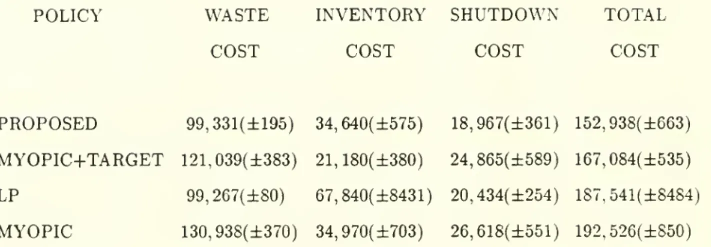
POLICY

WASTE

INVENTORY

SHUTDOWN

TOTAL

COST

COST

COST

COST

PROPOSED

99,331(±195) 34,640(±575) 18,967(±361) 152,938(±663)

MYOPIC+TARGET

121,039(±383) 21,180(±380) 24,865(±589) 167,084(±535)

LP

99,267(±80) 67,840(±8431) 20,434(±254) 1S7,541(±8484)

MYOPIC

130,938(±370) 34,970(±703) 26,618(±551) 192.526(±850)

TABLE

III. Simulation Results: Average

Annual

Costs.

The

simulation results are reported in Table III, which contains the average total

an-nual cost,

and

its

breakdown

into inventory (holding

and

backorder), waste

and shutdown

costs;

95%

confidence intervals are reported for all cost quantities. Notice that paper waste accounts for roughly two-thirds of the total cost. For ease ofcomparison. Table l\ reports

average costs as a percentage of the costs of the

PROPOSED

policy.

the accuracy ofour derived values for 5

and

S, a two-dimensional search

was

undertaken

for the cost minimizing values.

The

search yielded an average annual cost of $149,932, which is less than

2%

lower than the cost under our derived values. However, the cost

minimizing values, s

=

—17.5

and

S

=

175.0, are significantly different than the derived

values, s

=

—39.74

and

S

=

211.17. Consequently, the cost minimizing s

and

S

resulted

in lower inventory costs

and

higher

shutdown

costs relative to the derived values of .s

and

5; its four normalized costs for Table

IV

are 100%,

75%,

131%

and

98%.

The

cost minimizing value of 7 in (59)-(60)

was

0.9.

The

PROPOSED

policy's

per-formance

was

remarkably robust with respect to this parameter.

The

average total cost

increased by

0.3%

when

7

=

0.95

and

increased by less than 0.2%i

when

-;

=

0.7.

We

also tested the

PROPOSED

policy under one slight variant: the (s,S) policy

was

based

on

the total unweighted inventory _^j^-i Zk{t) rather than the weighted inventory

^j(._j ini.Zk{t).

A

searchforthe best {s,S)policy gaveessentially the

same

cost ($150,037)

as the search under the weighted inventory policy ($149,932). This close agreement is

hardly surprising since the three mjt values are very similar. Hence, any discrepancy

among

the various policies cannot be attributed to the fact that the

PROPOSED

policy

bases its _(5,5) policy on the weighted inventory,

and

the other policies base their (s.S)

policy

on

the unweighted inventory.

As

expected, the

LP

policy achieves the

same

waste cost as the

PROPOSED

policy.

However, since the

LP

policy is an

open

loop policy (i.e., the cutting policy is independent

of the state of the system), very high inventory costs are incurred.

The

cost minimizing

values of s

and

S

are 5

=

—15,000 and

S

=

235,000. Recall that i;

and

S

are expressed

in imits of hours for the

PROPOSED

policy,

and

in units of

pounds

of paperfor theother three policies.

The

MYOPIC

policy achieves the worst performance of the fovir policies. Since the

MYOPIC

and

PROPOSED

policies have similar inventory costs, it appears that the

in-ventory cost reductions gained by the

MYOPIC

policy while the

machine

was operating 24

were offset during the

shutdown

periods. Moreover, since the

MYOPIC

poHcy

employs

activities that do not minimize average waste costs, a significant increase in waste cost

is incurred. Finally, the high backorder cost incurred during the long

shutdown

periods

forces this policy to

employ more

frequent shutdowns

and

hence incur higher

shutdown

costs.

The

cost minimizing values of s

and

S

are s

=

—50,000,

5

=

100, 000.

For both

myopic

policies, the cost minimizing value of u), which is the

maximum

allowable waste

on

a paper roll,

was

found to be 2.75", which

was

the lowest value that

included any activities producing product 3. This parameter value allowed ten cutting

configurations to be employed.

When

w

was

raised to 3.0", two

more

activities were included

and

the overall cost increased by

6.3%

for the

MYOPIC

pohcy

and

9.49c for the

MYOPIC+TARGET

policy.

When

w

was

raised to the next levelof 4.75". eight additional

activities were included for a total of 20,

and

the cost roughly doubled for both policies.

The

use of the target inventory levels clearly enhances performance, since the

MY-OPIC+TARGET

policy achieves a

much

lower cost than the

MYOPIC

policy.

The

MY-OPIC+TARGET

policy achieves significantly lower inventory costs than the other three

policies. However, relative to the

PROPOSED

policy, thiscost reduction is

more

than offset

by increased waste

and

setup costs.

We

were initially

somewhat

surprised that the

PRO-POSED

poHcy, which uses only three activities, outperformed the

MYOPIC+TARGET

policy, which can

employ

any

number

of activities; after all, the primary- reason for

re-stricting the

number

of cutting configurations was to obtain a mathematically tractable

problem.

The

discrepancy in performance between these two pohcies can best be seen

by

comparing

the

MYOPIC+TARGET

policy to the

PROPOSED

policy under the cost

minimizing values (as opposed to the derived values) of 5

and

S: the two policies have

identical

shutdown

costs, the

PROPOSED

policy has

21.8%

higher inventory costs than

the

MYOPIC+TARGET

policy,

and

the

MYOPIC+TARGET

policy has 21.9% higher

waste costs than the

PROPOSED

policy. Hence, the

11%

difference in average total cost

between the two policies is due to the fact that waste costs comprise roughly two-thirds of

thetotal cost. Therefore, sincewaste costs are minimizedin thefirst step ofour procedure, the

PROPOSED

poHcy

may

not

work

as well

when

wastecosts are small relative to

inven-tory

and shutdown

costs. However,

we

reiterate that the problem parameters

employed

in

this simulation study are based

upon

our best estimates

from

aji actual facility.

It is worth noting that not only does the

PROPOSED

policy outperform the other

three policies in the simulation study, but it is also simpler to

employ

than the other

policies. First, the

PROPOSED

poHcy

is based

on

derived values of s

and

S, whereas the other policies require a two-dimensional search using a simulation model. Furthermore, the

PROPOSED

policy's performance is very robust with respect to the parameter 7,

which specifies the proximity toshutdown. In contrast, the performanceof the two

myopic

policies

was

very sensitive to the parameter w, which is the

maximum

allowable waste per

roll. Hence, the parameter 7 is

much

easier to specify than the parameter w.

6.

Other

Applications

In this section,

we

briefly describe several other settings

where

the two-step procedure

may

be applicable.

Semiconductor Manufacturing. In semiconductor wafer fabrication, a batch ofwafers produced according to a particular process

randomly

yields chips of

many

different

prod-uct types, which are partially ordered with respect to quality. Here, Fi,j rejjresents the

expected

number

of type k chips in a batch of wafers produced according to process j.

These facilities usually have

many

more

possible production processes than product types.

Each

production process has its

own

variable cost,

and

costlier processes will typically yield higher quality chips.

The

LP

in the first step of the procedure minimizes average

variable processing cost subject to meeting average

demand.

Wafer

fabrication facilities often operate in a make-to-stock

mode

and

often have only one bottleneck station, the photoHthography workstation,

and

wafers visit this station ten to twent}- times during

processing. Hence, by focusing on the bottleneck workstation,

we

obtain a scheduling 2G

problem

for a production/inventory system with customer feedback

and

random

yield.

The

Browniaji control

problem

in the second step of the procedure

was

expUcitly solved

in

Ou

and

Wein

(1992)

and

readers are referred there for details. Similar problems also

occur in fiber optics, ingot

and

crystal cutting,

and

blending operations in the petroleimi

industry.

Blood

Separation.

A

variety of separation processes can be used to separate blood

into its various

components

(plasma, red blood cells, etc.), which are maintained in a finished goods inventory servicing hospitals

and

other health care facilities. Here, each separation process has its

own

variable cost, which are minimized in the first step LP,

and

produces specific

amounts

of each component.

One

key aspect that is not captured in our

model

is the perishability of the blood; typically, blood

components

(except for plasma)

have to be discarded after sitting in inventory for a certain

number

of days.

Steel Industry. In a tube mill, each product type can be

made

from several different

blooms, or starting stocks,

and

a particular starting stock can be used to produce several

different products. If

we

define an activity for each feasible combination of starting stock

and

product type, then the activity cost includes both

raw

material costs for the starting

stock

and

processing costs, which differ by activity.

The

second step analysis develops a

dynamic

production policy for the bottleneck operation ofthe tube mill.

Acknowledgments

We

are deeply indebted to

Tim

Loucks, plant

manager

at Strathmore Paper

Company,

for generously sharing his time

and

expertise.

We

also thank

Anant

Balakrishnan for

engaging in helpful conversations about the steel industry. This research

was

partially

supported by a grantfrom the Leadersfor Manufacturing

Program

at

MIT

and

by National Science Foundation Grant

Award

No.

DDM-9057297.

REFERENCES

Bather, J. 1966.

A

Continuous

Time

Inventory Model. J. Applied Probability 3,

538-549.

Courcoubetis,

C,

P. Konstantopoulos, J. Walrand,

and

R. R. Weber. 1989.

Stabi-lizing an Uncertain Production System.

Queueing

Systems 5, 37-54.

Courcoubetis, C.

and

U. G.

Rothblum.

1991.

On

Optimal

Packing of

Randomly

Arriving Objects.

Mathematics

of Operations Research 16, 176-194.

European

Journal of Operations Research 44, 133-306, 1990.

Harrison, J.

M.

1988.

Brownian Models

of

Queueing

Networks with Heterogeneous

Customer

Populations, in

W.

Fleming

and

P. L. Lions (eds.), Stochastic

Differ-ential Systems, Stochastic Control

Theory

and

Applications.

IMA

Volume

10, Springer- Verlag,

New

York. 147-186.

Johnson. H. T.

and

R. S. Kaplan. 1987. Reievance Lost:

The

Rise

and

Fall of

Management

Accounting. Harvard Business School Press, Boston.

Krichagina, E.V.. S. X. C. Lou. S. P. Sethi

and

M.

I. Taksar 1992a. Production

Control in a Failure-Prone Manufacturing System: Diffusion .-Approximation

and

Asymptotic

Optimalitj'. Submitted for publication.

Krichagina, E. V.. S. X. C.

Lou and M.

I. Taksar 1992b.

Double

Band

Policy for

Stochastic Manufacturing Systems in

Heavy

Traffic. Submitted for publication.

Miller, B. L. 1974. Dispatching

from

Depot

Repair in a Recoverable Item Inventory System:

On

the Optimality of a Heuristic Rule.

Management

Science 21. 316-325.

Ou,

J.

and

L.

KL

Wein. 1992.

Dynamic

Scheduling of a Production/Inventory

Sys-tem

with By-Products

and

Random

Yield. Submitted to

Management

Science.

Puterman.

M.

L. 1975.

A

Diffusion Process

Model

for a Storage System. In

Logif'-tics,

M.

A. Geisler, ed., North-Holland,

Amsterdam,

143-159.

Veatch,

M.

H.

and

L.

M.

Wein. 1992. Scheduling a Make-to-Stock Queue: Index

Policies

and Hedging

Points. Technical Report, Operations Research Center,

MIT.

Wein, L.

M.

1992.

Dynamic

Scheduling ofa Multiclass Make-to-Stock Queue.

Op-erations Research 40, 724-735.

Zipkin, P. 1990.

An

Alternative

Dynamic

Scheduling Pohcy.

Working

notes, Grad-uate School of Business,

Columbia

Univ.,

New

York.

'...-

^ -. 29

Date

Due

MIT lIBRARirS Dlini