Developing Foram-AMBI for biomonitoring in the Mediterranean: Species
assignments to ecological categories
Frans Jorissen
a,⁎, Maria Pia Nardelli
a, Ahuva Almogi-Labin
b, Christine Barras
a, Luisa Bergamin
c,
Erica Bicchi
a,d, Akram El Kateb
e, Luciana Ferraro
f, Mary McGann
g, Caterina Morigi
h,i,
Elena Romano
c, Anna Sabbatini
j, Magali Schweizer
a, Silvia Spezzaferri
e aLPG-BIAF UMR CNRS 6112, University of Angers, 2 Boulevard Lavoisier, 49045 Angers Cedex 01, FrancebGeological Survey of Israel, Malkei Israel Street 30, Jerusalem 95501, Israel
cISPRA, Institute for Environmental Protection and Research, Via V. Brancati, 60, 00144 Rome, Italy dESAIP La Salle Graduate School of Engineering, 18, Rue du 8 mai 1945, 49180 St. Barthélemy d'Anjou, France eUniversity of Fribourg, Department of Geosciences, Chemin du Musée 6, 1700 Fribourg, Switzerland
fCNR, Institute for Coastal Marine Environment, National Research Council of Italy, Calata Porta di Massa, Naples, Italy gU.S. Geological Survey, Pacific Coastal and Marine Science Center, 345 Middlefield Road, MS 999, Menlo Park, CA 94025, USA hDepartment of Earth Sciences, University of Pisa, Via Santa Maria, 53, 56126 Pisa, Italy
iDepartment of Stratigraphy, Geological Survey of Denmark and Greenland (GEUS), Copenhagen, Denmark jUniversità Politecnica delle Marche, Dipartimento di Scienze della Vita e dell'Ambiente, Ancona, Italy
Most environmental bio-monitoring methods using the species composition of marine faunas define the Ecological Quality Status of soft bottom ecosystems based on the relative proportions of species assigned to a limited number of ecological categories. In this study we analyse the distribution patterns of benthic for-aminifera in the Mediterranean as a function of organic carbon gradients on the basis of 15 publications and
assign the individual species tofive ecological categories. Our categories (of sensitive, indifferent and 3rd, 2nd
and 1st order opportunists) are very similar to the ecological categories commonly used for macrofauna, but show some minor differences. In the 15 analysed publications, we considered the numerical data of 493 taxa, of
which 199 could be assigned. In all 79 taxa were classified as sensitive, 60 as indifferent, 46 as 3rd order, 12 as
2nd order and 2 as 1st order opportunists. The remaining 294 taxa are all accessory, and will only marginally contribute to biotic indices based on relative species proportions. In this paper we wanted also to explain the methodology we used for these species assignments, paying particular attention to all complications and pro-blems encountered. We think that the species list proposed here will constitute a highly useful tool for for-aminiferal bio-monitoring of soft bottoms in the Mediterranean Sea, which can be used in different ecological indices (Foram-AMBI and similar methods). With additional information becoming available in the next few years, it will be possible to expand the list, and, if necessary, to apply some minor corrections. As a next step, we intend to test this species list using several biotic indices, in a number of independent data sets, as soon as these will become available.
1. Introduction
The increasing concern for marine ecosystem health has led to a strong demand for suitable bio-indicator methods, capable of quanti-tatively assessing the quality of marine habitats and the biotic response to various types of anthropogenic impact. In Europe, this demand is even stronger because of two decisions of the European Community, which enforce member states to define the Ecological Quality Status (EQS) of their marine water bodies. The European Water Framework
Directive (WFD, 2000/60/EC) obliges all countries to achieve a good status of all water bodies, including marine waters up to one nautical
mile offshore, by 2015. Similarly, the Marine Strategy Framework
Directive (MFSD, 2008/56/EC) aims to obtain Good Environmental Status (GES) for Europe's marine waters by 2020.
Because of these far-reaching decisions, a large number of mon-itoring tools have been developed. It is important not only to evaluate the physico-chemical characteristics of the concerned water bodies, but also the eventual impact of eutrophication, pollutants and physical
⁎Corresponding author.
E-mail address:[email protected](F. Jorissen).
http://doc.rero.ch
Published in "Marine Micropaleontology 140 (): 33–45, 2018"
which should be cited to refer to this work.
disturbance on the living biota. In order to do so, several bio-indicators have been developed. For soft-bottom marine habitats, macrofauna is traditionally used as a bio-indicator of EQS, and a wide range of
dif-ferent biotic indices have been developed (overview in Borja et al.,
2016). Among these, many are based on the relative proportions of
indicator species (e.g.,Word, 1979; Bellan, 1980; Bellan-Santini, 1980;
Roberts et al., 1998; Borja et al., 2000; Gomez Gesteira and Dauvin, 2000; Eaton, 2001; Smith et al., 2001; Simboura and Zenetos, 2002).
Most of the biotic indices using macrofauna are based on changes in faunal composition and/or biodiversity in response to organic
enrich-ment, due to the different ecological strategies of the concerned species.
The underlying thought is that although anthropogenic pollution may have many aspects (such as different chemical pollutants), an increased organic load introduced into the marine environment can be considered as a common trait. In more extreme cases, increased oxygen demand may lead to the development of hypoxia at the sediment-water inter-face. It is implicitly assumed that the faunal response to organic en-richment, eventually accompanied by hypoxia, is representative for most types of pollution.
Therefore, in most macrofaunal indices, macrofaunal taxa are
clas-sified as a function of their response to enrichment, either in a rather
arbitrary way, or on the basis of more or less elaborated statistical
procedures (e.g.,Hily, 1984; Glémarec et al., 1986; Borja et al., 2000;
Rosenberg et al., 2004; Muxika et al., 2007). In most of these biotic indices, the relative proportions of a number of previously defined ecological groups are used to quantitatively define the EQS. At present,
the AZTI Marine Biotic Index (AMBI,Borja et al., 2000) is probably the
most commonly used. It is largely based on the early works ofGlémarec
and Hily (1981),Hily (1984)andGrall and Glémarec (1997), and uses five different ecological groups.
The use of meiofauna, occurring in substantially higher densities, is
much less developed (Kennedy and Jacoby, 1999). Among these,
benthic foraminifera (BF) appear particularly suitable for bio-mon-itoring. BF faunas typically contain high numbers of individuals in small areas (typically hundreds to thousands of individuals per
100 cm2), present high species diversity, with various microhabitats
and ecological niches being occupied and individual species showing a wide range of reactions to anthropogenic impact. Because of their short
life spans (3 months to 2 years;Murray, 1991), they react very rapidly
to anthropogenic disturbance, and thus give an integrated picture for a relevant period of time. Most importantly, the shells of most species are preserved in the sediment, thus offering the possibility of reconstructing the historical development of pollution, and obtaining a more precise idea of base-line conditions and faunas.
The international FOraminiferal BIoMOnitoring (FOBIMO) Group, a consortium of scientists developing the use of foraminifera as bio-in-dicators, was founded in 2011, with the objective of developing a standardised foraminiferal biomonitoring tool, and making it available
to a wider community. As a first step, a standardised protocol was
proposed for sampling and sample treatment (Schönfeld et al., 2012).
The next step was to develop a standardised biotic index based on foraminifera.
Since the AMBI-index is widely used for macrofauna, easy to apply,
and apparently yields coherent results (e.g.,Salas et al., 2004; Muniz
et al., 2005; Muxika et al., 2005; Hutton et al., 2015), the FOBIMO-Group decided to investigate the possibility of adapting this index to foraminifera. During the early stages of this process, it appeared that individual species might not show the same response to organic
en-richment in different climatologic and oceanographic settings. For this
reason, four working groups were created, studying NE Atlantic and Arctic ecosystems, transitional environments, tropical environments and Mediterranean ecosystems, respectively. The working group con-cerned with NE Atlantic and Arctic ecosystems presented the
Foram-AMBI index (Alve et al., 2016), and tested it by comparing the
Foram-AMBI scores with organic carbon content (TOC) and Shannon diversity in four independent data sets.
This paper presents the first results of the working group on
Mediterranean ecosystems. Because of the particular characteristics of their habitats (high temperature and salinity, overall oligotrophy con-trasting with coastal eutrophication), Mediterranean faunas may have different ecological requirements than Atlantic faunas, maybe related to some cryptic endemicity. Consequently, there was a consensus that at
thefirst stage, ecological species assignments should be limited to the
Mediterranean area, and should be exclusively based on observations made within the Mediterranean. At a later phase, it will be interesting to compare species assignments between the Mediterranean and other basins, in order to investigate whether ecological strategies of
in-dividual species are indeed different between basins, and if so, whether
these differences are important.
Evidently, the assignment of individual species to various ecological groups is crucial for all biotic indices, which use the relative
propor-tions of these groups to quantitatively define the EQS. In most previous
studies, species assignments to ecological groups have been made ra-ther arbitrarily, more or less based on expert knowledge, for
macro-fauna as well as for foraminifera (e.g.,Borja et al., 2000; Dimiza et al.,
2016). The aim of the FOBIMO-Group was to base the species
assign-ments on the objective study of a maximal number of suitable data sets, whereby assignments of individual taxa are made as a function of their distribution along well described organic enrichment gradients.
In the paper ofAlve et al. (2016), which introduces the Foram-AMBI
index, the process of species assignment was done as described in the previous paragraph, but is not described in great detail. Here, we pre-sent a list with 223 taxa occurring in the Mediterranean, which we have
assigned tofive ecological groups, on the basis of a careful study of 15
data sets. We wanted especially to show in detail: 1) how individual species were assigned to the ecological groups, and 2) the complications we encountered, which made this process sometimes particularly dif-ficult. We think that the species list presented here is the best result that can be obtained today, on the basis of an objective study of published data. However, additional data sets will become available in future, and will allow assigning more species, and eventually, apply some moderate corrections. The validation of Foram-AMBI using the species list pre-sented here, and the comparison of the Atlantic and Mediterranean species lists are objectives for further studies.
2. Criteria for the foraminiferal data sets used in this study The aim of this study was to describe the behaviour of Mediterranean BF taxa in response to various levels of natural and/or anthropogenic organic enrichment. Among the many published articles dealing with the recent ecology of BF faunas in the Mediterranean, we retained only 15 studies for the assignment of species to ecological categories. Our selection was based on three main criteria: 1) the pre-sence of a gradient in organic carbon content, 2) the nature of the studied samples (living, dead or total faunas), and additionally 3) the availability of grain size data.
Since sediment organic carbon content is probably the most prac-tical descriptor of organic enrichment, we decided to use only data sets in which this parameter had been measured. In fact, sediment organic carbon is also used as an environmental reference parameter for
bio-monitoring methods using macrofauna (e.g.,Borja et al., 2003).
Living BF faunas mirror present environmental conditions (e.g.,
Schönfeld et al., 2012), whereas total faunas (live + dead individuals)
tend to give an averaged picture for a (much) longer period (Murray,
1982). For this reason, we decided that our ecological species
assess-ments had to be based as much as possible on benthic foraminiferal biocoenoses. However, in the Mediterranean, living (Rose Bengal stained) faunas have only been collected over the last 25 years, and
studies of living assemblages are still rare, and often do not include organic carbon data.
Sediment grain size is another important parameter controlling BF
distribution in marine environments (e.g.,Basso and Spezzaferri, 2000;
Celia Magno et al., 2012). It is not necessarily sediment grain size itself
that influences BF faunas, but a complex of other factors related to it,
such as organic content, pore water oxygen concentration, vegetation,
current velocity (e.g.,Jorissen, 1987). Unfortunately, grain size has
only rarely been quantified in BF ecological studies. Nevertheless, we
privileged data sets including this parameter.
Only eight data sets found in the literature on recent Mediterranean foraminifera respected the two main criteria retained for this study: living faunas and organic carbon data. In order to increase the number of data sets, seven supplementary studies were added, in spite of the fact that one of the two conditions was not respected. In fact, the studies of Jorissen (1988), Samir and El-Din (2001), Hyams-Kaphzan et al. (2008),Romano et al. (2009, 2013)andFerraro et al. (2012)are all based on total faunas. Nevertheless, in view of the size of the respective data sets, and the presence of reliable organic carbon measurements for all stations, we expected that these studies would add essential in-formation about the ecological preferences of many Mediterranean BF
species. The same holds for the study ofErnst et al. (2005), which is
based on a laboratory experiment.
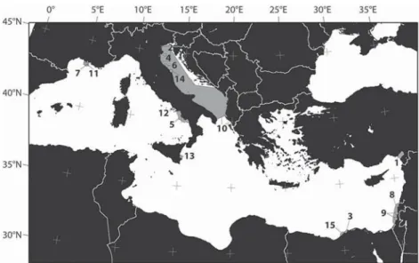
Allfifteen retained studies (Fig. 1,Table 1, Appendix A) concerned
open marine shelf environments, some of them in supposedly
un-polluted environments, with natural Corg gradients, and others in
clearly polluted settings. For all studies, only samples with a minimum of 40 specimens have been considered for further analysis. A more detailed description of the 15 retained data sets is added as supple-mentary material (Appendix A).
Careful inspection of Table 1reveals some major methodological
differences between the 15 studies. Probably the most important bias in
the data sets is due to different methods to measure organic carbon
content; this topic is further discussed inSection 4.4. Unfortunately, the
large majority of the studies are based on samples taken with Van Veen grabs, which presents the risk of losing part of the more or less liquid
superficial sediment (Schönfeld et al., 2012). For the studies based on
living foraminifera, different Rose Bengal concentrations and staining
periods have been used.
Concerning size fraction, about half of the studies are based on
the > 63μm fraction, the others on the > 125 μm or > 150 μm
frac-tion. We think that in spite of these differences, ecological responses to
organic carbon gradients can be perceived in all studies. However, it is evident that opportunistic reactions or sensitivity to increased organic
input of small-sized species can only be observed in studies of
the > 63μm fraction.
3. Ecological groups
In this study, we have classified the BF taxa in five ecological groups,
with different responses to organic enrichment (Fig. 2). A similar
sub-division has been used in many previous studies dealing with macrofauna.
Thefive ecological groups traditionally used for macrofauna (sensitive,
indifferent, tolerant, 2nd and 1st order opportunists) are largely based on
the faunal successions described in the classical study ofPearson and
Rosenberg (1978)around the sewage dump site in the Firth of Clyde, and
have been summarised byGrall and Glémarec (1997).Borja et al. (2000)
implemented them in their widely used AMBI-index.
Initially, the FOBIMO-Group attempted to use the samefive
ecolo-gical categories for BF. However, the ecoloecolo-gical patterns revealed in the
19 studies considered byAlve et al. (2016), and the 15 studies
pre-sented here, suggested that the definitions of some of the groups were
not entirely satisfying for BF. For this reason, slightly modified, more
precise descriptions of the five groups were presented byAlve et al.
(2016). In order to avoid confusion with the ecological groups
de-scribed for macrofauna (e.g., Grall and Glémarec, 1997; Borja et al.,
2000), we decided to change the name of the third category from
“Tolerant” to “3rd order opportunists” (Fig. 2). We think that this new
name better describes the distributional pattern of this group. Examples
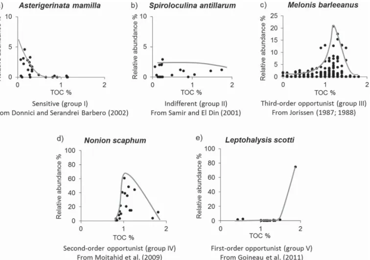
for each of thefive groups are presented inFig. 3.
Group I contains all“Sensitive species”. This concerns taxa which
are (very) sensitive to organic enrichment, and mainly occur in natural, oligotrophic, unpolluted ecosystems. This group of species is prominent at the reference site(s), where natural conditions are found, char-acterised by low to moderate organic matter contents. It disappears, or shows a clear decrease (ideally in absolute as well as relative abun-dance) in case of increasing organic enrichment. The concerned species are absent at strongly enriched sites. This group contains many different taxa, with individual species mostly being present with low relative densities (below 2%). Unfortunately, it is very difficult to observe clear trends for species occurring with such low relative densities, and con-sequently, many rare species which probably belong to this group, could not be assigned.
Group II consists of“Indifferent species”. These species are
in-different to the first stages of organic enrichment, but disappear in case
of (strongly) increased organic supplies. They tend to be present with fairly low relative densities, and do not show a clear trend in absolute and/or relative abundance towards moderately enriched sites.
Fig. 1. Map showing the 15 previous studies on Mediterranean BF ecology used in this paper. 1.Basso and Spezzaferri, 2000; 2.Donnici
and Serandrei Barbero, 2002; 3.Elshanawany et al., 2011; 4.Ernst
et al., 2005; 5.Ferraro et al., 2012; 6.Frontalini et al., 2011; 7.
Goineau et al., 2011; 8.Hyams-Kaphzan et al., 2008; 9.
Hyams-Kaphzan et al., 2009; 10.Jorissen, 1988; 11.Mojtahid et al., 2009;
12.Romano et al., 2009; 13.Romano et al., 2013; 14.Sabbatini et al.,
2012; 15.Samir and El-Din, 2001.
Table 1 Overview of the 15 studies used in this paper, with an indication of the sampling area and period, water depth range, sampling tool, staining method, st udied size fraction, the nature of the studied samples (living, dead or total faunas), the number of samples taken into account for the assignment and the method used to determine OC contents. Article Location/sampling period
Water depth range
(m) Sampling device/ sampled interval Staining treatment/mesh sieve Assemblage No. of considered samples TOC method TOC range variations Comments Basso and Spezzaferri, 2000 . Turkey-Iskenderun Bay/June 1993 7– 85 10 l Van Veen Grab/ 0– 2c m 4% formalin solution with sea water bu ff ered with 20 g o f Na2B4O7/l and 2 g Rose Bengal/63 μ m Living (Rose Bengal stained) 18 Loss on ignition 2.7 –15.8% Donnici and Serandrei Barbero, 2002 Italy-Northern Adriatic continental shelf/July –August 1996 5– 46 Van Veen grab & box corer (total association) & box corer (living association)/0 –7c m 1 h in a Rose Bengal and ethanol solution 5 g 1 l l/wet sieving 63 μ m; dry sieving > 125 μ m Living (Rose Bengal stained) and total 25 Elemental analyser (Mod 2400) 0.07 –1.15% Elshanawany et al., 2011 Egypt-Abu-Qui Bay/ May –November 2005 0.83 –8.8 Grab/0 –3 cm Solution Rose Bengal and ethanol/63 μ m Living (Rose Bengal stained) 9 Carbon analyser (C-200, version 2.6) 0.1 –5.9% Ernst et al., 2005 Italy-Northern Adriatic Sea/ February 2000 32 Van Veen Grab/ 0– 3c m NA/500 μ m Living NA Elemental analyser Fison NA 1500 NCS Experimental research on living BF in oxic/anoxic conditions Ferraro et al., 2012 Italy-Southern Tyrrhenian continental shelf/ October –November 2003 12 –195 Van Veen Grab/ 0– 5c m NA/ > 6 3 and 125 μ m Total assemblage 72 Elemental analyser ThermoElectron Flash EA 1112 0.33 –5.73% Frozen samples Frontalini et al., 2011 Italy-Adriatic Sea/coast along Gabice-Pesaro-Fano/ May –July 2002 5– 13 15 l Van Veen Grab/ upper centimetres Solution of Rose Bengal and ethanol (2 g/l)/ > 6 3 μ m Living (Rose Bengal stained) 6 Loss on ignition 3– 13% Dried at 60 °C for 6 h Goineau et al., 2011 France-Gulf of Lion/ August –September 2006 15 –100 Barnett multicorer/ 0– 1c m Solution of Bengal Rose and ethanol (1 g/l)/ > 125 μ m Living (Rose Bengal stained) 20 CN analyser LECO 2000 0.43 –2.10% Hyams-Kaphzan et al., 2008 Israeli coast/1996 –1999 3– 40 Scuba diving 3– 30 (bulk sediment sample) and Box core (40 m depth)/0 –5c m Solution of Bengal Rose and ethanol (2 g/l)/ > 6 3 and 149 μ m Total assemblage 57 Modi fi ed Walkley-Black titration 0.1 –1.0% TOC measures made in 2011 Hyams-Kaphzan et al., 2009 Israel-near Palmahim/ January 2003 –May 2004 34 and 36 Box core (BX 700 AL)/ 0– 5 and 0– 10 cm Solution of Rose Bengal and ethanol (2 g/l)/ > 6 3 μ m Living (Rose Bengal stained) 23 Elemental analyser, EA-1112 unit (combustion at 1750 °C) 0.3 –16% TOC on dry sediments, acid-decarbonated and oven dried at 50 °C before the analysis. Also Chlorophyll data and porewater O2 are available Jorissen, 1988 Italy-Adriatic Sea/1962 7.5 –302 Grab/0 –4 cm NA/ > 150 μ m Total assemblage 249 Loss on ignition 0 and 1.5% Mojtahid et al., 2009 France-Gulf of Lion/June 2005 20 –98 Bowers and Connelly Mark VI multicorer/ 0– 5c m Rose Bengal (1 g/l)/and ethanol solution/ > 6 3 and 150 μ m Living (Rose Bengal stained) 33 CHN Elementary analyser 0.82 –1.91% Dried at 50 °C, homogenized. Romano et al., 2009 Italy, Gulf of Pozzuoli/ November –December 2004 3.3 –58.3 Van Veen Grab/ 0– 2c m Rose Bengal (1 g/l)/and ethanol solution/ > 6 3 μ m
Total assemblage (living
+ dead) 37 CHNS-O EA 1110 Thermo Electron 0.01 –19.41% Dried; treated with HCl Romano et al., 2013 Italy, Sicily-Augusta Harbour/ 2005 Mean 14.9 Van Veen Grab/ 0– 2c m Rose Bengal (1 g/l)/and ethanol solution/ > 6 3 μ m
Total assemblage (living
+ dead) 37 Loss of ignition at 450 °C 0.21 –10.07% Dried sediment Sabbatini et al., 2012 Italy-Adriatic Sea (Ancona)/ May, July, October 2008 15 Van Veen Grab/ 0– 1c m 10% formalin solution with sea water bu ff ered with Na2B4O7/l and 2 m l o f Rose Bengal/ > 6 3 and 150 μ m Living (Rose Bengal stained) 4 Fluorimetry (Chl-a ) and spectro-photometry (BCP) 1.6 –17.5 μ g/g Chl-a ; 0.6 –1.96 mg/g BCP BCP = sum of lipids, proteins and carbohydrates (bioavailable C). Samples stored at − 20 °C until investigated. Only used to classify L. scottii (continued on next page )
http://doc.rero.ch
Group III is composed of“Third-order opportunists”. This cerns species which are present at the reference sites, in natural
con-ditions, which are tolerant to thefirst stages of organic enrichment, and
are relatively favoured by such conditions, as is shown by their abun-dance increase (absolute as well as relative) towards more enriched areas. However, their density maximum is usually fairly distant from the areas of maximum enrichment, where they tend to be absent. The
species of this group have previously been labelled as“tolerant” (e.g.,
Grall and Glémarec, 1997; Alve et al., 2016). However, since the species of Group II are also tolerant to the early stages of ecosystem enrich-ment, and the species of Group III show a clear opportunistic response
to enrichment, we have preferred to name them“third-order
opportu-nists”.
Group IV consists of“Second-order opportunists”. These taxa are
absent, or occur in low frequency (< 2%) at the reference station(s), with natural conditions, and low to moderate organic matter content, and strongly increase towards sites of maximum organic enrichment, with maximum abundance between Groups III and V.
Group V is composed of“First-order opportunists”. These species
are also absent or rare (< 2%) at the reference site(s), their density strongly increases towards the organic enrichment source, but their maximum abundance is situated closer to the site(s) of maximum en-richment than species of the Group IV. These are the last species present
before azoic conditions are encountered (Fig. 2). Dense populations of
these highly opportunistic taxa can only be observed in strongly eu-trophicated areas.
During the analysis of individual data sets, we sometimes felt the need to use intermediate categories. This was for instance the case when we hesitated between two groups, or when we observed a clear opportunistic response, but it was difficult to determine where exactly the concerned station was situated along the overall enrichment
gra-dient. In the first case we used mixed categories (I–II, II–III, etc.),
whereas in the second case we indicated only the opportunistic
re-sponse by assigning a III–IV–V label. For the final assignments (Table 2,
Appendix C, right side), for each species all individual assignments (Appendix C, left side; for many species, assignments were available for more than one study) were carefully assessed, and each species was assigned to a single category, so that the intermediate categories dis-appeared.
Finally, in individual studies, a large number of taxa could not be
Table 1 (continued ) Article Location/sampling period
Water depth range
(m) Sampling device/ sampled interval Staining treatment/mesh sieve Assemblage No. of considered samples TOC method TOC range variations Comments Samir and El-Din, 2001 Egypt-El Mex and Miami Bays/March 1994 1– 19 Petterson grab/0 –2 cm 20% formalin solution and stain with bu ff ered Rose Bengal (1 g/l distilled water)/ >6 3 μ m Total assemblages 18 NA 0.22 –3.15% TOM published in El-Sabrouti et al. (1997)
Fig. 2. Conceptual graph showing the changes of the cumulative relative abundance of all species belonging to each of the 5 ecological groups along an organic enrichment gra-dient. Pristine natural conditions are situated on the left, increasingly enriched conditions are found towards the right, untilfinally azoic conditions are reached on the right of the diagram. See text for further explanation.
Source: Modified afterAlve et al., 2016.
assigned (NA in Appendix C). This was for instance the case when percentages were very low, when the species was only present in few samples, or showed strongly varying percentages without a clear trend.
4. Difficulties encountered in the analyses of the 15 data sets
While analysing the 15 selected data sets, complications of very
different nature have been encountered. Some of these issues concern
the comparison of sites within a single data set, whereas others concern the comparison of species distribution between different data sets. The
following seven subchapters will briefly discuss the main difficulties we
encountered.
4.1. Comparing sites with different substrate types
Most foraminiferal taxa have a preference for a particular type of substrate, some species prefer sandy sediments, whereas others prefer
a silty to clayey seafloor. In natural coastal settings, sediment grain
size tends to be strongly correlated with organic matter because,
especially infine-grained sediments, organic compounds may be
ad-sorbed on the surface of clay minerals (smectite, illite) and within the
clay mineral interlayers (e.g.,Kennedy et al., 2002). The consequence
is that in natural conditions, clayey sediments usually have a higher TOC content than sandy sediments. In natural conditions, BF faunas found on sandy sediments with low TOC contents usually have a high contribution of epiphytic/epifaunal taxa, which are generally
con-sidered as pollution-sensitive (e.g.,Barras et al., 2014). Conversely,
the faunas of clayey substrates often contain high proportions of
stress-resistant taxa (e.g.,Jorissen, 1987; Celia Magno et al., 2012).
In many nearshore settings, inner littoral sandy sediments present a rather sharp boundary with clayey sediments of a coast-parallel mud belt, which has developed in the Holocene on a global scale (e.g.,
Van der Zwaan and Jorissen, 1991). Onshore to offshore transect which cross this major biofacial limit will show a sudden increase in TOC, accompanied by an important shift in faunal composition, to-wards faunas with a higher percentage of stress-tolerant taxa. Of
course, this faunal shift mainly reflects a change in substrate type,
and not an increased anthropogenic enrichment. This observation clearly shows that the faunal successions along TOC gradients can only be correctly understood if sediment grain size is taken into ac-count. Preferably, the organic gradient under consideration should not be accompanied by a change in sediment grain size, although this is only rarely the case.
A clear example of this problem is given by Asterigerina adriatica in
the data set ofDonnici and Serandrei Barbero (2002). In fact, in this
data set, the transition from sand to clay bottoms coincides with a shift in TOC from values between 0.1 and 0.5% to values between 0.6 and
1.2% (Fig. 4). If we consider the whole range of TOC values, this species
would probably be classified as “indifferent” (Group II), since no clear
trend in relative abundance is visible in response to increasing %TOC. However, if we consider only the sandy substrates and no longer take into account changes induced by the abrupt change in sediment grain size at about 0.55% TOC, a clear positive correlation with TOC becomes evident, suggesting that this species is initially favoured by increased TOC values. Consequently, in this study, the species was classified as a 3rd order opportunist (Group III).
Fig. 3. Examples of species assigned to each of the 5 ecological groups. All data are taken from individual studies, which are indicated below each of thefive panels. The schematic enveloping curves indicate the maximum relative frequencies found as a function of %TOC, when all other conditions are optimal.
4.2. Taxonomical issues
The taxonomy of BF is complex. First, very different species and
genus concepts are used, some based on typological approach, with only a limited amount of morphological variability within the taxon, whereas others admit a much wider morphological range in a single species or genus. Next, various taxonomical schools still exist, which do not give the same taxonomical importance to some of the
morpholo-gical criteria. For instance, very different taxonomical schemes are used
for non-costate buliminids. Finally, some species names are only used regionally, also in cases where the endemic nature of the concerned species has never been shown. The consequence is that in many cases,
different species names are in use for what apparently is a single
spe-cies. In the last decades, molecular studies have partly solved some of
these problems (e.g., Hayward et al., 2004; Tsuchiya et al., 2008;
Darling et al., 2016), but much taxonomical confusion remains. In the case of this inventory of Mediterranean foraminifera, we tried as far as possible to avoid taking decisions in case of taxonomical dis-agreements. In cases where we thought that in the analysed papers,
different names were used for the same species, we systematically listed
the data of all papers under all species names used, leading to several entries for what is apparently a single species (for instance, Nonion
fabum and Nonion scaphum inTable 2and Appendix C). Only in a few
cases of evidently wrong determinations, which could only be re-cognised as such when SEM (Scanning Electron Microscope) photos were available, we allowed ourselves to correct the name. However, since many of the analysed papers did not present plates, this was only done in a very limited number of cases. A similar strategy was followed at the genus level; in case of more than one genus name used for the same species, all data were listed under both genus names (for instance,
Bolivina alata and Brizalina alata inTable 2and Appendix C). Appendix
B lists all taxa considered as synonymous (at the genus as well as the species level).
A final difficulty was the fact that in several of the investigated
studies, many taxa were listed in open nomenclature, without species name. In this case, it was impossible to compare species patterns be-tween studies. Details for such taxa can be found in Appendix C. In
Table 2, we decided not to list such taxa, with three exceptions.
Trilo-culinella sp. 1 (data fromHyams-Kaphzan et al., 2009) was added
be-cause it was attributed to ecological group IV, which has only few re-presentatives, and because it was the only representative of this genus. Fursenkoina sp. 1 and sp. 2 (of the same authors), which were attributed
to groups III and I, respectively, were added to show that not all re-presentatives of this genus have a distribution suggesting an opportu-nistic and/or stress-tolerant character.
4.3. Data on living faunas versus total/dead faunas
Most of the data sets we used are based on living (Rose Bengal
stained) faunas. However,five studies based on total faunas
(thanato-coenoses) were used as well, because of the very large data sets they contain. Living and total faunas do not give exactly the same in-formation. The living fauna represents a snapshot in a particular en-vironmental context that may vary considerably over short timescales. Conversely, total assemblages give an averaged picture for a much longer period of time (years to centuries), and their composition has
been transformed by taphonomical losses (e.g.,Murray and Alve, 1999;
Denne and Sen Gupta, 1989; Jorissen and Wittling, 1999). This con-cerns especially agglutinated taxa, many of which are rapidly
decom-posed after the death of the organisms (Bizon and Bizon, 1985;
Schröder, 1988). However, taphonomical processes may also affect
various taxa with calcareous tests, with important interspecific
differ-ences (Murray, 1991). In spite of these taphonomic losses, which
be-come more severe towards deeper sediment layers, total faunas still may contain useful ecological information, as is shown by the abundant use of fossil assemblage composition in paleoceanographical studies. As explained before, because of the scarceness of suitable data sets on
living foraminifera, we decided to addfive studies based on total
as-semblages in the topmost cm of the sediment. However, in these cases, all samples were critically scrutinised, and those with an indication of important taphonomical changes (bad preservation, reworked speci-mens, uncommonly high densities, etc.) where removed from the data sets before further examination.
4.4. Different methods for organic matter content measurements
Marine sediments often contain a mixture of organic carbon from terrestrial and marine sources. Organic matter in aquatic systems is a complex mixture of molecules such as carbohydrates, amino acids, hydrocarbons, fatty acids and phenols, natural macromolecules and colloids, originating from living phytoplankton and other plant mate-rial, soil organic matter, faunal remains, sewage and industrial dis-charge. There are numerous methods to quantify OM content, two of which are most often used: elemental analysis, and the loss on ignition
method (e.g., Buchanan, 1984). While the first method (i.e., TOC
measurement) is more accurate and has been widely documented (e.g.,
Luczak et al., 1997), the loss of weight on ignition method is still largely used in benthic ecology because it is quick and cheap, although it has a
larger analytical error, especially in clayey sediments (e.g.,Mook and
Hoskin, 1982).
Table 1shows that, generally, TOC determined by elemental ana-lysis yields maximal values of 1 to 5%, whereas in the loss on ignition method, maximum values are above 10%. It appears therefore that there is a strong methodological bias, and consequently, the TOC data of the 15 data sets cannot be compared at face value.
4.5. Abundant plant and algae debris leading to high TOC values Organic carbon compounds in the marine environment have three
main sources:fluvial supply of particulate organic matter, nearshore
production of benthic plants and algae, and phytoplankton production. The various organic compounds are more or less labile, and have widely varying nutritional values for benthic organisms. Consequently, several methods have been proposed to describe the bioavailability of organic
matter (e.g.,Dauwe and Middelburg, 1998; Grémare et al., 2003). It is
generally assumed that most BF taxa depend mainly on labile, easily
metabolisable organic matter (e.g.,De Rijk et al., 2000; Mojtahid et al.,
2009). It is evident, that in our data set, the TOC values will present a
Fig. 4. Relative abundance of Asterigerinata adriatica vs. TOC%, data fromDonnici and
Serandrei Barbero (2002). The diagram includes all the studied samples. Black symbols
indicate samples from sandy sediments, grey symbols samples from muddy sediments.
mixture of various types of organic matter, possibly with very different nutritional values. We suspect that the very high TOC values found in some of the data sets (more than one order of magnitude higher than
usual (e.g.,Basso and Spezzaferri, 2000) are not only due to a
metho-dological bias (elemental analysis versus loss on ignition, see previous paragraph), but may be caused by the presence of abundant remains of macroalgae and Posidonia. This hypothesis is corroborated by the abundant presence of epiphytic species in many of the samples. Such organic remains have probably a low nutritional value for foraminifera, and therefore, in these cases the high TOC values are probably not in-dicative of a food-enriched environment. Consequently, species found with high percentages in these samples are not favoured by enrichment, but are rather associated with macroalgae, for instance because of their epiphytic lifestyle. It is clear that preferences or absences of species at sites, with high TOC values due to phytal macrodetritus, should not be interpreted as a response to ecosystem eutrophication. All data sets have been scrutinised very carefully for this potential bias.
4.6. Comparing naturally eutrophicated and polluted areas
Another potential problem is the fact that the analysed data sets represent a mixture of studies of natural sites, without evident an-thropogenic pollution, and sites from polluted areas, some of them even strongly polluted. In both types of setting, the BF response to varying TOC concentrations is used to characterise the various species, and to attribute them to one of the ecological categories. However, there is a fundamental difference between natural and anthropogenically en-riched sites. In most natural ecosystems, organic enrichment is not accompanied by chemical pollution. Therefore, samples from naturally enriched sites basically show a faunal response to organic enrichment (and eventually hypoxia/anoxia) alone. Conversely, at polluted sites, organic supplies are usually accompanied by a more or less wide range of toxic chemical compounds, and the faunas potentially show a re-sponse to a multiple stressor context. In many cases of anthropogenic pollution there is a positive correlation between TOC and the
con-centrations of chemical pollutants (e.g.,Romano et al., 2009, 2013and
byElshanawany et al., 2011), and TOC values can be used as an in-tegrative descriptor of pollution. However, in some studies, the corre-lation between TOC and other pollutants is much less evident (e.g.,
Samir and El-Din, 2001), and TOC may not be a good descriptor for ecosystem stress. Such different situations may explain the observed
differences in faunal behaviour between sites with comparable TOC
values.
4.7. Positioning the data sets on the overall organic enrichment gradient
Thefinal problem we encountered was the position of each of the
investigated data sets along the ecological continuum used to define the
five ecological groups (Fig. 2), which extends from pristine natural
environments to sites which are so heavily enriched, that BF have disappeared. Although natural environments may be enriched in
or-ganic matter, especially when they are under strongfluvial influence,
eutrophication will not attain the same levels as in sites with strong anthropogenic pollution, such as sewage outlets, drill mud disposal sites or harbours. Since advanced stages of organic enrichment only rarely
develop in natural coastal sites, it is highly improbable tofind maximal
percentages of the opportunistic species of ecological categories IV and V (2nd and 1st order opportunists), or even more extreme azoic con-ditions. Most cases of opportunistic species responses in natural en-vironments concern type III species (3rd order opportunists). In order to take into account this complicated factor, all 15 data sets were very carefully evaluated, and we attempted to define for each study its range along the overall organic enrichment, and made species assignments accordingly.
5. Constructing the master table
Initially, each of the 15 data sets was studied independently by at least two researchers, who, whenever possible, assigned species to the five ecological categories in function of the relationship between their relative frequencies and TOC, eventually using the intermediate
cate-gories, as explained inSection 3. Next, the results of thesefirst analyses
were presented in a plenary session (FOBIMO Meeting, 28–30 October
2014, Angers), where each species assignment has been motivated and discussed, in order to verify that the same criteria had been used in all studies. This resulted in a spreadsheet with all individual species as-signments made in the 15 studies (Appendix C, left side).
The next step was to assign each individual species to an ecological category on the basis of a comparison and careful appreciation of the data of all studies in which the species was identified. This resulted in
thefinal “Master Table” (Table 2, Appendix C, right side). InTable 2,
only thefinal assignments are listed, whereas all detailed information is
given in Appendix C, for assigned as well as non-assigned taxa. When comparing the results for all 15 data sets, a wide range of
different situations were encountered, for instance:
1) All individual species assignments (Appendix C, left side) agreed,
and the assigned ecological category was retained for the final
Master Table. Examples are Peneroplis planatus, Bolivina sub-aenariensis and Quinqueloculina agglutinans.
2) Some species (e.g., Miliolinella semicostata or Textularia conica) could only be assigned unambiguously in a single study, which was con-sidered sufficient for a final assignment.
3) In some cases, the species could not be assigned in any of the 15 studies (because of an absence of a clear pattern, or very low
den-sities), and thefinal assignment was NA (Not Assigned). This was for
instance the case for Elphidium pulvereum, Amphistegina lobifera and Pyrgo elongata. Such species are absent in the list of assigned species (Table 2) but are listed in Appendix C.
4) The species could be assigned in several studies, but not in other ones, because the pattern was not clear enough. In such cases the ultimate assignment (Appendix C, right side) was based on the studies in which the species could be assigned. This was for instance the case for Haynesina depressula, Ammonia beccarii and Adelosina mediterranensis.
5) Other species, such as Ammonia parkinsoniana, Cibicides lobatulus or Miliolinella subrotunda, could be classified in a large number of
studies, but often with slightly different results. In such cases, we
generally privileged data sets which showed the clearest trends, either decreasing percentages (sensitivity) or increasing percentages towards higher TOC (opportunistic response to enrichment). The most typical cases were:
a. The individual assignments of a species varied from sensitive (group
I) to indifferent (group II). Since we decided to privilege the clearer
trends, we assigned such taxa to group I. Examples are Planorbulina mediterranensis, Miliolinella subrotunda and Cibicides lobatulus.
b. The individual assignments varied from indifferent (group II) to
opportunistic (group III). As in the previous case, the more explicit trends were privileged, and such species were generally placed in category III. This was for instance the case for Bulimina marginata, Porosononion granosum and Bolivina seminuda.
6) In some rare cases we were faced with contradictive assignments, with a species showing a sensitive behaviour in some studies, and an opportunistic behaviour in other ones. In such cases we generally
decided to place the species in category II (indifferent species) or III,
in function of the position of the studied data set on the overall
enrichment scale (seeSection 4.7).
7) For several genera, some species could, but others could not be as-signed, mostly due to low relative densities and/or non-diagnostic
Table 2
List of the 256 taxa (including 33 synonyms) which have been assigned to ecological categories. The asterisks in the left column indicate species listed under several names, which are considered synonymous here. These synonyms are listed in Appendix B.
Synonyms Taxa Final assignment
Adelosina cf. carinatastriata 1 Acostata mariae 3 Adelosina cliarensis 1 Adelosina longirostra 1 Adelosina mediterranensis 1 Adelosina spp. 1 Adercotryma glomeratum 2 Affinetrina planciana 2 Agglutinella compressa 2
Ammonia beccari f. inflata 2
Ammonia beccarii 2 Ammonia compacta 3 * Ammonia falsobeccarii 3 * Ammonia inflata 2 * Ammonia parkinsoniana 1 * Ammonia perlucida 3 Ammonia tepida 4 Ammoscalaria foliaris 2 Amphicoryna scalaris 2 Amphistegina radiata 1 * Articulina mucrunata 1 * Asterigerinata adriatica 3 Asterigerinerata mamilla 1 Astrononion stelligerum 1 Aubignyna perlucida 3 Bigenerina nodosaria 2 Biloculinella labiata 2 Bolivina aenariensis 2 Bolivina alata 2 Bolivina catanensis 1 Bolivina difformis 2 Bolivina dilatata 2
Bolivina dilatata spathulata 1
Bolivina pseudoplicata 2 Bolivina seminuda 3 Bolivina spathulata 3 Bolivina striatula 3 Bolivina subaenariensis 2 * Bolivina variabilis 2 Brizalina alata 2 Brizalina difformis 2 Brizalina laevigata 3 Brizalina striatula 3
Buccella frigida granulata 1
Buccella granulata 1 Buccella pustulosa 2 Bulimina aculeata 3 Bulimina costata 2 * Bulimina denudata 4 * Bulimina elongata 3 Bulimina gibba 3 Bulimina marginata 3 Caronia silvestrii 3 * Cassidulina carinata 4 * Cassidulina laevigata 4 * Cassidulina oblonga 2 Cibicidella variabilis 1 * Cibicides lobatulus 1 Cibicides refulgens 1 Clavulina cylindrica 3 Cornuspira involvens 3 Coscinospira hemprichii 1 Cribroelphidium oceanensis 3 Cribroelphidium poeyanum 3 Cycloforina contorta 1 Cycloforina polygona 2 Cycloforina quinquecarinata 1 Discorbinella bertheloti 1 Discorbis bertheloti 1 Discorbis mirus 1 Eggerella scabra 3 Eggerelloides advenus 3 Table 2 (continued)
Synonyms Taxa Final assignment
Eggerelloides scaber 3 * Elphidium aculeatum 1 * Elphidium advenum 2 * Elphidium complanatum 1 * Elphidium crispum 1 Elphidium decipiens 2 Elphidium depressulum 2 Elphidium granosum 3 Elphidium lidoensis 2 Elphidium macellum 1 Elphidium poeyanum 3 Elphidium punctatum 2 Elphidium striatopunctatum 1 Elphidium translucens 2 Epistominella vitrea 4 Eponides concameratus 1 Eratidus foliaceus 2
Fissurina orbignyana caribaea 2
* Fursenkoina sp. 1 (Hyams-Kaphzan et al., 2009) 3 Fursenkoina sp. 2 (Hyams-Kaphzan et al., 2009) 1
* Gavelinopsis praegeri 1 * Gavelinopsis translucens 1 Glabratella erecta 1 Glabratella hexacamerata 1 Globobulimina affinis 2 Globocassidulina subglobosa 2 Globotextularia anceps 1 * Globulina gibba 1 * Guttulina lactea 3 Guttulina problema 2 Gyroidina umbonata 2 Haynesina depressula 2 Haynesina germanica 3 * Heterostegina depressa 1 * Hopkinsina pacifica 3 Hyalinea balthica 2 Lachlanella planciana 2 Lachlanella variolata 1 Laevipeneroplis karreri 2 Lagenammina atlantica 2 Lagenammina difflugiformis 2 * Lagenammina fusiformis 3 Leptohalysis scottii 5 Lobatula lobatula 1 Massilina paronai 2 Massilina secans 2 Melonis barleeanus 3 Miliolinella labiosa 1 Miliolinella perplexa 3 Miliolinella semicostata 1 Miliolinella spp. 1 * Miliolinella subcircolaris 1 Miliolinella subrotunda 1 * Morulaeplecta bulbosa 3 * Neoconorbina posidonicola 1 Neoconorbina terquemi 1 Nonion depressulum 2 Nonion fabum 4 Nonion scaphum 4 * Nonionella atlantica 3 Nonionella opima 4 * Nonionella turgida 5 Nonionoides grateloupi 2 Nouria polymorphinoides 3 Nubecularia lucifuga 1 Nubeculina divaricata 1 Pararotalia calcariformata 1 Pararotalia spinigera 1 Peneroplis karreri 2 Peneroplis pertusus 1 Peneroplis planatus 1 Planorbulina mediterranensis 1 Planorbulina variabilis 1 Porosononion granosum 3 Porosononion subgranosum 3
(continued on next page)
patterns. In the case of Adelosina, Miliolinella and Rosalina, nearly all species which could be assigned confidently, and were mostly placed in group I (sensitive species). Since the less common species of these genera together showed also a distribution typical of group I, we supposed that they had similar ecological requirements. Therefore, for these two genera, we added an entry in the Master Table for the genus as a whole (e.g., Adelosina spp.). In this way, all rare species belonging to these genera were implicitly assigned as well.
8) When in individual studies, an opportunistic behaviour was ob-served, but we could not decide whether the concerned sites were moderately, strongly or extremely enriched in organic matter, we
initially considered these species only as“opportunistic”, and
as-signed them to a lump category“III–IV–V”. As usual, the final
as-signment of such species was made by comparing the asas-signments of all studies in which the species was found. Once again, in general the clearest responses were privileged, leading to assignments in the highest possible category.
According to the methodologies used and the range of environ-mental conditions, the observations on species distribution of some studies were considered as slightly more reliable compared to other ones. Reasons for this could be the fact that living (Rose Bengal stained) faunas had been studied, more samples had been considered, or the TOC gradient was larger. In cases of contradictory evidence for a given species, results from studies considered as more reliable were privi-leged. Finally, in spite of these general rules, in some rare cases it was extremely difficult to reach a decision on the basis of the available data, mostly because of the presence of clearly contradictory information. In
such cases, thefinal assignment was sometimes partly based on expert
knowledge, after extensive discussion in the general assembly. 6. The Master Table of ecological assignments
In the 15 investigated studies, 493 taxa (synonyms only counted once) had absolute and relative frequencies high enough to be considered. Of these, 199 could be classified in one of the five ecological categories (Table 2), because they showed at least in one study a clear response to organic enrichment, either in anthropogenic or naturally eutrophicated settings. The remaining 294 taxa occurred mostly with low relative fre-quencies, so that their contribution to most bio-indication methods based on relative taxon frequencies is probably rather limited.
Of the 199 taxa which could be classified:
•
79 have been placed in ecological group I (sensitive)•
60 in ecological group II (indifferent),•
46 in group III (3rd order opportunists)•
12 in group IV (2nd order opportunists), and•
2 in group V (1st order opportunists).Species which were determined under different names in the fifteen investigated studies have been listed two (or more) times in the Master Table 2 (continued)
Synonyms Taxa Final assignment
Pseudoeponides falsobeccarii 3 Pseudotriloculina brongniartiana 2 * Pseudotriloculina laevigata 2 * Pyrgo oblonga 2 Quinqueloculina agglutinans 1 Quinqueloculina agglutinata 1 Quinqueloculina annectens 1 Quinqueloculina aspera 1 Quinqueloculina auberiana 1 * Quinqueloculina badenensis 3 Quinqueloculina bosciana 2 * Quinqueloculina bradyana 2 * Quinqueloculina candeiana 2 Quinqueloculina contorta 1 * Quinqueloculina costata 1 Quinqueloculina disparilis 1 Quinqueloculina inaequalis 2 * Quinqueloculina laevigata 1 Quinqueloculina lata 3 * Quinqueloculina milletti 1 Quinqueloculina padana 3 Quinqueloculina parvula 2 Quinqueloculina pygmaea 3 Quinqueloculina seminula 3
* Quinqueloculina seminula f. longa 4
Quinqueloculina seminulum 3
Quinqueloculina seminulum f. longa 4
Quinqueloculina stelligera 3 * Quinqueloculina subpolygona 1 * Quinqueloculina tenuicollis 4 Quinqueloculina tropicalis 4 * Quinqueloculina viennenis 2 * Quinqueloculina vulgaris 1 * Rectuvigerina phlegeri 3 Recurvoides trochamminiformis 2 Reophax fusiformis 3 Reophax nana 3 Reophax scorpiurus 2 * Reophax scotti 5 Reussella spinulosa 1 Rosalina bradyi 1 * Rosalina candeiana 1 Rosalinafloridana 1 Rosalina globularis 1 * Rosalina macropora 1 Rosalina obtusa 2 * Rosalina spp. 1 * Sigmoilina costata 1 Sigmoilina edwarsi 2 * Sigmoilinita costata 1 Sigmoilopsis schlumbergeri 3 * Siphonaperta agglutinans 1 * Siphonaperta aspera 1 Sorites orbiculus 1 * Spirillina vivipara 3 * Spiroloculina angulata 1 * Spiroloculina antillarum 2 Spiroloculina dilatata 2 Spiroloculina excavata 1 Spiroloculina nummiformis 1 Spiroloculina rotundata 1 Spiroplectammina earlandi 2 Stainforthia complanata 3 Stainforthia fusiformis 3 Textularia agglutinans 3 Textularia bocki 3 * Textularia calva 3 Textularia conica 1 Textularia earlandi 2 Textularia truncata 1 Trifarina angulosa 2 Triloculina affinis 2 * Triloculina laevigata 1 * Triloculina marioni 2 Triloculina plicata 3 Table 2 (continued)
Synonyms Taxa Final assignment
* Triloculina schreiberiana 3
* Triloculina tricarinata 1
Triloculina trigonula 1
Triloculinella sp. 1 (Hyams-Kaphzan et al., 2009) 4
Trochammina globigeriniformis 2 Uvigerina mediterranea 2 * Uvigerina phlegeri 3 Valvulineria bradyana 4 * Vertebralina striata 1
http://doc.rero.ch
Table, but have only been counted once to obtain the numbers given above. This concerns for instance the 1st order opportunist Leptohalysis
scotti, which is also listed as“Reophax scotti”. Appendix B lists all
re-cognised synonyms occurring in the Master Table. 294 of the 493
considered taxa could not yet be classified, because of inconclusive
data. However, more suitable studies will doubtlessly become available in the future, which should ultimately make it possible to classify part of these taxa as well.
When on the basis of thefinal assignments, the appearances of
re-presentatives of the 5 groups are considered in each of the studies (Table 3), it appears that in most cases representatives of all ecological categories are present, including opportunistic Groups III, IV and V
(e.g.,Basso and Spezzaferri, 2000; Goineau et al., 2011). This suggests
that a rather complete ecological gradient has been sampled, from natural, non-enriched to heavily eutrophicated sites. In some studies, only very few representatives of Groups III, IV and V were observed.
This concerned the studies ofSamir and El-Din (2001),Hyams-Kaphzan
et al. (2008), Romano et al. (2009)andElshanawany et al. (2011). These studies apparently did not include heavily organic matter
en-riched sites. Conversely, the studies ofMojtahid et al. (2009),Frontalini
et al. (2011),Sabbatini et al. (2012), and, to a lesser degree,Goineau et al. (2011)contained only small numbers of Group I (and Group II) taxa, suggesting that all investigated stations were enriched in TOC, either naturally or anthropogenically, and that these studies lack the pristine, non-enriched side of the spectrum.
7. Discussion and perspectives
In this paper we present assignments of 199 common Mediterranean
BF taxa to 5 ecological categories. Thefinal list of species assignments is
the fruit of a very thorough and objective inspection of all existing Mediterranean BF data sets until 2014. We think that this list is an es-sential tool for all bio-indication methods, which use the relative pro-portions of stress-tolerant and/or stress-sensitive taxa to obtain a
quan-tified measure of the EQS, either by Foram-AMBI (Alve et al., 2016) or by
a comparable method (e.g.,Barras et al., 2014; Dimiza et al., 2016).
For macrofauna, very similar lists have been constructed. However, with the exception of the list used to define the Benthic Quality Index
(BQI,Rosenberg et al., 2004) which is defined in a very objective way,
the way most other species lists have been constructed is not very transparent. In view of the decisive importance of the species assign-ments to ecological categories, it appeared essential to us to present our list for Mediterranean species, together with a clear overview of how it was constructed, and of the many problems and complications which were encountered while constructing it. We think that it is important that all researchers who use such lists, realise that they are obtained by painstaking literature analyses, and unavoidably contain an element of subjectivity. The present list represents at best our current knowledge of Mediterranean BF ecology. Additional future studies will allow to complete it, and to apply corrections for some taxa, if needed.
As explained before, like most existing lists for macrofauna, our spe-cies assignment list is mainly based on the faunal response to organic matter enrichment, which is used as a descriptor for anthropogenic pol-lution. An important question is whether species which are resistant to, or even favoured by organic enrichment, are also tolerant to other pollu-tants. Since in marine ecosystems, stress parameters are mostly co-oc-curring, the answer to this question can probably only come from
ex-perimental studies (e.g.,Denoyelle et al., 2012; Nardelli et al., 2013).
Finally, after constructing this list, the next step is to test it on in-dependent data sets, containing also TOC measurements, either by
using Foram-AMBI (Alve et al., 2016) or similar methods (e.g.,Barras
et al., 2014; Dimiza et al., 2016). Another objective for further studies is the comparison of ecological assignments of Mediterranean and
Atlantic species (Alve et al., 2016). An important question is whether
the eventual differences between the two lists are due to different
re-sponses to organic enrichment in different climate regimes.
Table 3 Number of taxa fi nally assigned to each of the 5 ecological categories in each of the 15 studies. Basso and Spezzaferri, 2000 Donnici and Serandrei Barbero, 2002 Elshanawany et al., 2011 Ernst et al., 2005 Ferraro et al., 2012 Frontalini et al., 2011 Goineau et al., 2011 Hyams- Kaphzan et al., 2008 Hyams- Kaphzan et al., 2009 Jorissen, 1987, 1988 Mojtahid et al., 2009 Romano et al., 2009 Romano et al., 2013 Sabbatini et al., 2012 Samir and El-Din, 2001 Total assigned Group I 2 5 2 6 3 9 0 14 3 1 0 1 1 1 6 1 0 3 16 9 3 33 79 Group II 12 14 7 0 6 1 23 3 1 4 1 3 1 8 8 4 5 17 60 Group III 15 17 6 6 10 11 18 5 2 2 1 2 1 1 9 12 11 2 46 Group IV 2 4 1 1 4 1 8 1 3 5 5 0 3 2 2 12 Group V 1 0 0 1 0 1 2 0 1 1 2 0 0 1 0 2 Total assigned 55 61 53 8 3 4 1 7 6 1 2 0 5 6 4 1 3 9 3 3 2 8 2 2 5 4 199 Not assigned 23 49 5 0 0 2 37 5 3 7 1 1 1 7 1 2 5 16 294 Total no. of species 78 110 58 8 3 4 1 9 9 8 2 5 9 3 5 2 5 6 3 4 3 0 2 7 7 0 493
http://doc.rero.ch
Acknowledgements
We are very grateful to all members of the FOBIMO-group for many stimulating discussions. We especially acknowledge Elisabeth Alve, Sergei Korsun and Joachim Schönfeld, who commented on an earlier version of the manuscript. We thank the editor in chief Richard Jordan and two anonymous reviewers for their very constructive and useful comments.
Appendix A. Supplementary data
Supplementary data to this article can be found online athttps://
doi.org/10.1016/j.marmicro.2017.12.006. References
Alve, E., Korsun, S., Schönfeld, J., Dijkstra, N., et al., 2016. Foram-AMBI: a sensitivity index based on benthic foraminiferal faunas from North-East Atlantic and Arctic
fjords, continental shelves and slopes. Mar. Micropaleontol. 122, 1–12.
Barras, C., Jorissen, F., Labrune, C., Andral, B., Boissery, P., 2014. Live benthic for-aminiferal faunas from the French Mediterranean Coast: towards a new biotic index
of environmental quality. Ecol. Indic. 36, 719–743.
Basso, D., Spezzaferri, S., 2000. The distribution of living (stained) benthic foraminifera in Iskenderun Bay (Eastern Turkey): a statistical approach. Boll. Soc. Paleontol. Ital.
39, 359–380.
Bellan, G., 1980. Annélides polychétes des substrats solids de trois mileux pollués sur les côtes de Provence (France): Cortiou, Golfe de Fos, Vieux Port de Marseille. Tethys 9,
260–278.
Bellan-Santini, D., 1980. Relationship between populations of amphipods and pollution.
Mar. Pollut. Bull. 11, 224–227.
Bizon, G., Bizon, J.J., 1985. Distribution des foraminifères sur le plateau continental du
Rhône. ECOMED 84–94.
Borja, A., Franco, J., Pérez, V., 2000. A marine biotic index to establish the ecological quality of soft-bottom benthos within European estuarine and coastal environments.
Mar. Pollut. Bull. 40, 1100–1114.
Borja, A., Muxika, I., Franco, J., 2003. The application of a Marine Biotic Index to dif-ferent impact sources affecting soft-bottom benthic communities along European
coasts. Mar. Pollut. Bull. 46, 835–845.
Borja, A., Elliott, M., Andersen, J.H., Berg, T., Carstensen, J., Halpern, S., et al., 2016. Overview of integrative assessment of marine systems: the ecosystem approach in practice. Front. Mar. Sci. 3, 20.http://dx.doi.org/10.3389/fmars.2016. 00020.
Buchanan, J.B., 1984. Sediment analysis. In: Holme, N.A., McIntyre, A.D. (Eds.), Methods for the Study of Marine Benthos, 2nd ed. Blackwell Scientific Publications, Oxford,
pp. 41–64.
Celia Magno, M., Bergamin, L., Finoia, M.G., Pierfranceschi, G., Venti, F., Romano, E., 2012. Correlation between textural characteristics of marine sediments and benthic foraminifera in highly anthropogenically-altered coastal areas. Mar. Geol. 315–318,
143–161.
Darling, K.F., Schweizer, M., Knudsen, K.L., Evans, K.M., Bird, C., Roberts, A., Filipsson, H.L., Kim, J.H., Gudmundsson, G., Wade, C.M., Sayer, M.D.J., Austin, W.E.N., 2016. The genetic diversity, phylogeography and morphology of Elphidiidae (Foraminifera)
in the Northeast Atlantic. Mar. Micropaleontol. 129, 1–23.
Dauwe, B., Middelburg, J.J., 1998. Amino acids and hexosamines as indicators of organic
matter degradation state in North Sea sediments. Limnol. Oceanogr. 43, 782–798.
De Rijk, S., Jorissen, F.J., Rohling, E.J., Troelstra, S.R., 2000. Organicflux control on
bathymetric zonation of Mediterranean benthic foraminifera. Mar. Micropaleontol.
40, 151–166.
Denne, R.A., Sen Gupta, B.K., 1989. Effects of taphonomy and habitat on the record of
benthic foraminifera in modern sediments. PALAIOS 4, 414–423.
Denoyelle, M., Geslin, E., Jorissen, F.J., Cazes, L., Galgani, F., 2012. Innovative use of foraminifera in ecotoxicology: a marine chronic bioassay for testing potential toxicity
of drilling muds. Ecol. Indic. 12, 17–25.
Dimiza, M.D., Triantaphyllou, M.V., Koukousioura, O., Hallock, P., Simboura, N., Karageorgis, A.P., Papathanasiou, E., 2016. The Foram Stress Index: a new tool for environmental assessment of soft-bottom environments using benthic Foraminifera. A case study from the Saronikos Gulf, Greece, Eastern Mediterranean. Ecol. Indic. 60,
611–621.
Donnici, S., Serandrei Barbero, R., 2002. The benthic foraminiferal communities of the
North Adriatic continental shelf. Mar. Micropaleontol. 44, 93–123.
Eaton, L., 2001. Development and validation of biocriteria using benthic
macro-invertebrates for North Carolina estuarine waters. Mar. Pollut. Bull. 42, 23–30.
El-Sabrouti, M.A., Bader El-Din, A., El Samak, A., 1997. Textural and chemical char-acteristics of the surficial sediments in two coastal bays of Alexandria, Egypt. In: Proceedings of the Seventh International Conference on Environmental Protection,
Alexandria, pp. 118–130 (20-22 May).
Elshanawany, R., Ibrahim, M.I., Milker, Y., Schmiedl, G., Badr, N., Kholeif, S.A., Zonneveld, K.A.F., 2011. Anthropogenic impact on benthic foraminifera, Abu-Qir
Bay, Alexandria, Egypt. J. Foraminifer. Res. 41, 326–348.
Ernst, S., Bours, R., Duijnstee, I., van der Zwaan, B.D., 2005. Experimental effects of an organic matter pulse and oxygen depletion on a benthic foraminiferal shelf
com-munity. J. Foraminifer. Res. 35, 177–197.
Ferraro, L., Alberico, I., Lirer, F., Vallefuoco, M., 2012. Distribution of benthic for-aminifera from the southern Tyrrhenian continental shelf (South Italy). Rendiconti Fisici Accademia Lincei 23, 103–119.
http://dx.doi.org/10.1007/s12210-011-0160-2.
Frontalini, F., Semprucci, F., Coccioni, R., Balsamo, M., Bittoni, P., Covazzi-Harriague, A., 2011. On the quantitative distribution and community structure of the meio and macrofaunal communities in the coastal area of the Central Adriatic Sea (Italy). Environ. Monit. Assess. 180, 325–344.
http://dx.doi.org/10.1007/s10661-010-1791-y.
Glémarec, M., Hily, C., 1981. Perturbations apportées à la macrofaune benthique de la baie de Concarneau par les effluents urbains et portuaires. Acta Oecologica Oecologia
Applicata 2, 139–150.
Glémarec, M., Le Bris, H., Le Guellec, C., 1986. Modifications des écosystèmes des vasières cotières du sud-Bretagne. Hydrobiologia 142, 159–170.http://dx.doi.org/
10.1007/BF00026756.
Goineau, A., Fontanier, C., Jorissen, F.J., Lansard, B., et al., 2011. Live (stained) benthic foraminifera from the Rhône prodelta (Gulf of Lion, NW Mediterranean):
environ-mental controls on a river-dominated shelf. J. Sea Res. 65, 58–75.
Gomez Gesteira, L., Dauvin, J.C., 2000. Amphipods are good bioindicators of the impact of oil spills on soft-bottom macrobenthic communities. Mar. Pollut. Bull. 40,
1017–1027.
Grall, J., Glémarec, M., 1997. Using biotic indices to estimate macrobenthic community
perturbations in the Bay of Brest. Estuar. Coast. Shelf Sci. 44 (suppl. A), 43–53.
Grémare, A., Medernach, L., DeBovee, F., Amouroux, J.M., Charles, F., Dinet, A., Vetion, G., Albert, P., Colomines, J.C., 2003. Relationship between sedimentary organic matter and benthic fauna within the Gulf of Lion: synthesis on the identification of new biochemical descriptors of sedimentary organic nutritional value. Oceanol. Acta
26, 391–406.
Hayward, B.W., Holzmann, M., Grenfell, H.R., Pawlowski, J., Triggs, C.M., 2004.
Morphological distinction of molecular types in Ammonia– towards a taxonomic
revision of the world's most commonly misidentied foraminifera. Mar.
Micropaleontol. 50, 237–271.
Hily, C., 1984. Variabilité de la macrofaune benthique dans les milieux hypertrophiques
de la Rade de Brest. Thèse de Doctorat d'Etat. 1. Univ. Bretagne Occidentale, pp.
359 (Vol. 2: pp. 337).
Hutton, M., Venturini, N., Garcia-Rodriguez, F., Brugnoli, E., Muniz, P., 2015. Assessing the ecological quality status of a temperate urban estuary by means of benthic biotic
indices. Mar. Pollut. Bull. 91, 441–453.
Hyams-Kaphzan, O., Almogi-Labin, A., Sivan, D., Benjamini, C., 2008. Benthic for-aminifera assemblage change along the southeastern Mediterranean inner shelf due
to fall-off of Nile-derived siliciclastics. Neues Jb. Geol. Paläontol. Abh. 248, 315–344.
Hyams-Kaphzan, O., Almogi-Labin, A., Benjamini, C., Herut, B., 2009. Natural oligo-trophy vs. pollution-induced euoligo-trophy on the SE Mediterranean shallow shelf (Israel): environmental parameters and benthic foraminifera. Mar. Pollut. Bull. 58,
1888–1902.
Jorissen, F.J., 1987. The distribution of benthic foraminifera in the Adriatic Sea. Mar.
Micropaleontol. 12, 21–48.
Jorissen, F.J., 1988. Benthic foraminifera from the Adriatic Sea; principles of phenotypic
variation. Utrecht Micropaleontol. Bull. 37, 174.
Jorissen, F.J., Wittling, I., 1999. Ecological evidence from live-dead comparisons of benthic foraminiferal faunas off Cape Blanc (Northwest Africa). Palaeogeogr.
Palaeoclimatol. Palaeoecol. 149, 151–170.
Kennedy, A.D., Jacoby, C.A., 1999. Biological indicators of marine environmental health:
meiofauna - a neglected benthic component? Environ. Monit. Assess. 54, 47–68.
Kennedy, M.J., Pevear, D., Hill, R., 2002. Mineral surface control of organic carbon in
black shale. Science 295, 657–660.
Luczak, C., Janquin, M.A., Kupka, A., 1997. Simple standard procedure for the routine
determination of organic matter in marine sediment. Hydrobiologia 345, 87–94.
Mojtahid, M., Jorissen, F., Lansard, B., Fontanier, C., Bombled, B., Rabouille, C., 2009. Spatial distribution of live benthic foraminifera in the Rhône prodelta: faunal re-sponse to a continental-marine organic matter gradient. Mar. Micropaleontol. 70,
177–200.
Mook, D.H., Hoskin, C.M., 1982. Organic determinations by ignition, caution advised.
Estuar. Coast. Shelf Sci. 15, 697–699.
Muniz, P., Venturini, N., Pires-Vanin, A.M.S., et al., 2005. Testing the applicability of a Marine Biotic Index (AMBI) to assessing the ecological quality of soft-bottom benthic
communities, in the South America Atlantic region. Mar. Pollut. Bull. 50, 624–637.
Murray, J.W., 1982. Benthic foraminifera: the validity of living, dead or total assemblages
for the interpretation of palaeoecology. J. Micropalaeontol. 1, 137–140.
Murray, J.W., 1991. Ecology and Palaeoecology of Benthic Foraminifera. Longman
Scientific & Technical, Essex (UK) (397 pp).
Murray, J.W., Alve, E., 1999. Taphonomic experiments on marginal marine foraminiferal assemblages: how much ecological information is preserved? Palaeogeogr.
Palaeoclimatol. Palaeoecol. 149, 183–197.
Muxika, I., Borja, A., Bonne, W., 2005. The suitability of the Marine Biotic Index (AMBI)
to new impact sources along European coasts. Ecol. Indic. 5, 19–31.
Muxika, I., Borja, A., Bald, J., 2007. Using historical data, expert judgement and multi-variate analysis in assessing reference conditions and benthic ecological status,
ac-cording to the European Water Framework Directive. Mar. Pollut. Bull. 55, 16–29.
Nardelli, M.P., Sabbatini, A., Negri, A., 2013. Experimental chronic exposure of the