HAL Id: hal-00316242
https://hal.archives-ouvertes.fr/hal-00316242
Submitted on 1 Jan 1997
HAL is a multi-disciplinary open access archive for the deposit and dissemination of sci-entific research documents, whether they are pub-lished or not. The documents may come from teaching and research institutions in France or abroad, or from public or private research centers.
L’archive ouverte pluridisciplinaire HAL, est destinée au dépôt et à la diffusion de documents scientifiques de niveau recherche, publiés ou non, émanant des établissements d’enseignement et de recherche français ou étrangers, des laboratoires publics ou privés.
Small scale observation of magnetopause motion:
preliminary results of the INTERBALL project
J. Safrankova, G. Zastenker, Z. Nemecek, A. Fedorov, M. Simersky, L. Prech
To cite this version:
J. Safrankova, G. Zastenker, Z. Nemecek, A. Fedorov, M. Simersky, et al.. Small scale observation of magnetopause motion: preliminary results of the INTERBALL project. Annales Geophysicae, European Geosciences Union, 1997, 15 (5), pp.562-569. �hal-00316242�
Small scale observation of magnetopause motion:
preliminary results of the INTERBALL project
J. Safrankova1, G. Zastenker2, Z. Nemecek1, A. Fedorov2, M. Simersky1, L. Prech1
1
Faculty of Mathematics and Physics of Charles University, Prague, Czech Republic
2Space Research Institute, Academy of Sciences of Russia, Moscow, Russia
Received: 12 December 1995 / Revised: 14 October 1996 / Accepted: 16 October 1996
Abstract. Two satellites of the INTERBALL project
were launched on 3 August 1995. The main goals of the present paper are (1) to give a brief information about the VDP plasma device onboard the INTERBALL-1 satellite, (2) to present the Faradays cup data taken in different magnetospheric regions and (3) to expose first results of the two satellite measurements of the magne-topause motion. The presented data illustrate magneto-pause crossings as seen by two satellites when separated by about ~ 1000 km. This separation combined with the Faraday’s cup time resolution allows to estimate the velocity of the magnetopause and to reconstruct a possible structure of the boundary. Simultaneous mea-surement of the magnetic field supports the interpreta-tion of the observed ion fluxes as a signature of the wavy motion of the boundary.
1 Introduction
The position of the dayside and the near–Earth magnetotail magnetopause reflects the changes in the interplanetary magnetic field (IMF) and of the solar-wind parameters. The empirically derived curves ob-tained by Roelof and Sibeck (1993) and Petrinec and Russell (1993) are in good agreement with the observed magnetopause crossings despite the fact that the date sets for external values of the solar-wind pressure or the IMF are rather small. The spread of the experimental points around the theoretical curve is caused by a variety of transient events which divert the magneto-pause from its stationary position.
Transient (~ 1-min) events are a common feature of the outer dayside magnetosphere. Sibeck (1995) links such events to a number of processes, including multiple rapid magnetopause crossings, brief increase in the field component normal to the magnetopause and short enhancements of the ambient field strength. This author notes that this set of transient events includes what has been referred to as flux transfer events (FTEs) (by
Russell and Elphic (1978), who interpreted FTEs as evidence of patchy, sporadic merging resulting in the formation of flux ropes of interconnected magneto-sheath and magnetospheric magnetic field lines. Since magnetic merging requires the appearance of a magnet-ic-field component normal to the magnetopause, the events may be interpreted in terms of flux ropes or bubbles produced by merging pulses. Because opposed magnetosheath and magnetospheric magnetic-field ori-entations favour the occurrence of magnetic merging, flux-transfer events should be more common on the low-latitude dayside magnetopause during periods of south-ward interplanetary magnetic field.
Some authors believe that many of the observed transient events can be explained by changes of the solar-wind pressure and by the consequent magneto-pause motion and/or deformation. Sibeck et al. (1989a,b) and Fairfield et al. (1990) compared in detail high time-resolution observations taken upstream of the subsolar bow shock with magnetic-field observations made in the outer dayside magnetosphere. Their com-parison shows that transient magnetospheric events can be associated in a nearly one-to-one manner with equally transient variations in the foreshock dynamic pressure and in the IMF orientation. Le et al. (1993) interpreted the transient magnetospheric events as pressure-pulse-driven wavelets on the magnetopause.
The pressure pulses deform the magnetopause and create either crests or troughs on the surface (Sibeck et
al., 1990). The Kelvin-Helmholtz instability can further
cause the deformation of this boundary (Ogilvie and Fitzenreiter, 1989) and can lead to a large uncertainty in the magnetopause position determination.
It must be stressed that measurements made at one point in space are not sufficient for the determination of the shape of such a dynamic boundary object as the magnetopause.
In this paper we use preliminary results of simulta-neous measurements carried out by the two INTER-BALL satellites to contribute to the discussion on the origin of the transient events seen at the magnetopause.
Our results demonstrate the possibilities offered by satellites which are closely located and move in a similar orbit. Our conclusions are based on simultaneous measurements of the VDP plasma sensor onboard the INTERBALL-1 satellite and of the corresponding VDP-S sensor measurements on the MAGION–4 sub-satellite.
2 Instrumentation
The omnidirectional plasma sensor VDP is designed to determine the integral flux vector and the integral energetic spectrum of ions and electrons in the 0.2 – 2.4- keV energy range. For simultaneous measurements in all directions the VDP device is equipped with six independent wide-angle Faraday’s cups (FCs). Their axes form a three-dimensional orthogonal system. This configuration permits to find the main flow directions even in highly turbulent regions.
Measurements with FC are widely applied; they have been used several times onboard the Prognoz-type satellites for the solar wind (Gringauz et al., 1974; Vaisberg et al., 1979; Zastenker et al., 1982) and for the plasmasphere investigation (Vaisberg et al., 1979). The possibility to determine fast changes of the ion-flow direction by a system of FCs in the bow-shock region has been illustrated by Kozak et al. (1985). This method can supply the plasma velocity vector with a high temporal resolution. An illustration of these advantages can be found in Avanov et al. (1984), where fast fluctuations of the ion flow in the solar wind are measured with a time resolution of 20 ms.
As opposed to the solar wind, for magnetospheric measurements the full spatial coverage is of principal importance. As the period of rotation of the Prognoz-type spacecraft is about 2 min, the rotation cannot be used for fast spatial scanning and the sensor must cover the whole space to obtain a sufficient temporal resolu-tion. For this reason a set of six FCs was chosen, with the axes forming a three-dimensional orthogonal sys-tem. Moreover, the multisensor system will be very useful for the study of the counterstreaming flows which can be expected within magnetospheric boundaries.
2.1 Sensor design and characteristics
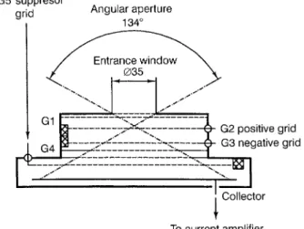
The main design characteristics of an FC are schemat-ically shown in Fig. 1. The entrance grid (G1) is connected to the cup body (and accordingly to the satellite body) for the protection of the environmental space from the influence of the device potentials. The next two grids (G2, G3) are used for selection of the registered particles according to the energy and the sign of their charge.
One of the following modes of operation can be chosen by command:
– measurement of the sum of total ion flux and flux of electrons with energy greater than 2.4 keV;
– measurement of the sum of flux of electrons with energy greater than 0.17 keV and of flux of ions with energy greater than 2.4 keV;
– measurement of the sum of the integral energy spectrum of ions in the range 0.2–2.4 keV and the flux of electrons with energy greater than 2.4 keV; – measurement of the sum of the integral energy
spectrum of electrons in the range 0.2–2.4 keV and the flux of ions with energy greater than 2.4 keV; – calibration of the amplifiers.
According to these modes the grids G2, G3 are supplied with potentials (relative to the body) shown in Table 1. The G4 grid is connected with the body to protect the collector (C) from the G3 potential influence. The suppressor grid G5 eliminates or diminishes the photo-electron and secondary photo-electron currents from the collector. It is supplied permanently with the negative voltage (–170 V). This potential exceeds considerably the possible energy of secondary electrons and photo-electrons arising under the action of the Sun’s UV radiation. During the calibration mode the triangular voltage is super-imposed on the DC suppressor voltage. Due to the capacitance between the grid and the collector, some signal appears at the collector and is used for the amplifier-gain determination. It should be mentioned that in the sensor oriented towards the Sun the G3 grid is connected with the body in order to avoid the production at G3 of photoelectrons with energy up to 2.4 keV (i.e. considerably more than the potential of the grid G5) which could reach the collector.
Fig. 1. Schematic of the sensor
Table 1. G2 and G3 grid potential
Mode of measurement U(G2)[kV] U(G3)[kV]
Ion flux 0 )2.4
Electron flux + 2.4 0 Spectrum of step voltage )2.4
ion flow + 0.2/ + 2.4
Spectrum of + 2.4 step voltage electron flow )0.2/) 2.4 Calibration + 2.4 )2.4 J. Safrankova et al.: Small scale observation of magnetopause motion: preliminary results of the INTERBALL project 563
The size of the collector, diameters of apertures and distances between the grids (see Fig. 1) are chosen so that the angular characteristics of the sensor have a triangular shape with width ±67°degrees. Under typical magnetospheric conditions the ion flow is registered by three sensors simultaneously. Based on the current ratios the uncertainty of the angle determination does not exceed a few degrees (e.g. Avanov et al., 1984).
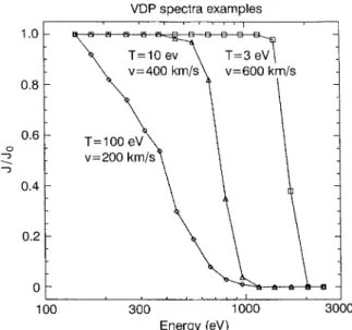
A sequence of retarding potentials is supplied to the G2 or G3 grids for the measurement of the integral energetic spectrum of particles. The whole energy range (0.2–2.4 kV) is divided logarithmically into 16 steps which are scanned each second. The sensor retarding characteristic was determined numerically, taking into account the real grid electric field. An example of the expected data calculated for three values of the plasma bulk velocity and temperature using this retarding characteristic is shown in Fig. 2. It can be seen that such integral energetic spectra can be used for a simple but rather good estimation of the velocity and temperature of the plasma flow with the assumption that the bulk velocity exceeds considerably the thermal one.
Measurements illustrated in Fig. 3 have been taken in the solar wind. They demonstrate a good agreement with predicted curves in Fig. 2. The velocity and temperature estimated from these measurements are 458 km/s and 12 eV, respectively. The difference between calculated and measured curves in the high-energy part is caused by thea-particle flux which is only one order of magnitude less than that of the protons. Three consec-utive measurements depicted in Fig. 3 show a good reproducibility of measurements of the proton part of the distribution. The part which corresponds to the a-particle distribution is rather noisy but averaging allows to determine also the basic parameters of thea-particle flow.
2.2 Sensor electronics
In accordance with our knowledge of interplanetary and magnetospheric plasma, the expected range of particle flux is from 3 × 10⁵ to 2× 10⁹part/cm2/s. Taking into account the entrance area of 9.6 cm2and the transpar-ency of the grid set of about 0.6, the corresponding current range is from 3×10–13to 2×10⁻⁹A. It is rather difficult to cover that range in one scale because of the noise level on the spacecraft. For this reason the whole range was divided into two subranges, two decimal orders each. The switching of the FC amplifier gain proceeds automatically in accordance with the input signal. The amplifier is complemented by a precise rectifier. The system provides three signals: analogue output, digital indication of the gain value and polarity. The frequency bandwidth of the amplifier reaches about 10 Hz. It gives a good opportunity to study turbulent magnetospheric plasma. To obtain this fre-quency and current ranges, the amplifier is placed just under the FC. The analogue output of the amplifier is passed through the low-pass filter (Butterworth type, second order) with an upper limit frequency of 8 Hz. This limit is in agreement with Nyquist criterion as the sampling rate of the data processing unit is 16 Hz.
2.3 Onboard data processing system
There are two basic features which characterize the VDP instrument data processing:
– The data processor unit (DPU) is used mainly for data processing, data compression and telemetry frame forming. All other activities such as control signals reception, timing, data collection and pre-processing are carried out by a dedicated hardware. It allows us to transmit the information to the telemetry system (TM) even if the DPU is switched off (e.g. within the Earth’s radiation belts). In these cases, information is sent to the particular TM via a parallel TM channel.
Fig. 2. Integral energy spectra calculated for three values of the bulk
velocity and temperature of an axial proton flow
Fig. 3. Example of measured integral energy spectra of a solar-wind
– All computations are carried out in bytes. To obtain the needed range, logarithmic data representation has been chosen and original algorithms and procedures have been developed for data processing and com-pression to reach the needed accuracy.
The main cycle of data collection is either 1 or 1/128 of the spacecraft revolution. The way of the synchroni-zation can be changed by a command from the Earth. During the cycle each of the six FCs is multiplexed 16 times to the input of a logarithmic AD converter. The output of the logarithmic ADC is written to the data buffer together with housekeeping and checking infor-mation, such as the phase of satellite rotation, sensor temperature and grid voltages. At the beginning of each cycle a restart signal for the DPU is generated and the data buffer is rewritten to the DPU memory.
The main tasks of the DPU can be listed as follows: – determination of the way the data should be
pro-cessed in accordance with received commands, – data processing and compression,
– computation of precursors of different plasma dis-turbances,
– telemetry frame formation,
– adaptive change of the telemetry bit rate and of the level of data compression.
Besides the tasks listed there are many other routines which can be commanded from the Earth and allow reprogramming or checking of the DPU.
Due to the spacecraft limitations, the most informa-tive mode – real-time transmission – can be expected only for limited parts of the orbit. For all other times the information must be written to the telemetry memory; which for our device cannot exceed 10 MB. To have a complete coverage of the orbit, the following modes are combined in accordance with scientific tasks.
– fast mode (430 kB/h) – the complete scientific information is transmitted with maximal rate; – fast monitoring mode (30 kB/h) – mean value for 1
from each sensor is transmitted together with the housekeeping data;
– slow monitoring mode (3.5 kB/h) – 8-s averages and housekeeping information are transmitted:
– adaptive mode (up to 430 kB/h). This mode can be started from both monitoring modes. The main idea is that if some disturbance in plasma is observed and if one or both precursors computed in the DPU exceed a given threshold, the actual mode is changed to the fast mode.
Further details and references are given in Safrankova
et al. (1995).
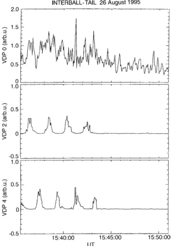
As an example of the data received in the fast monitoring mode we present the bow-shock crossing which occurred on 26 August 1995, when the satellite moved from the dawn magnetosheath into the solar wind at a distance of about 24.2 RE from the Earth
(Fig. 4). The magnetosheath ion flow is nearly antisun-ward in this region, but due to its high temperature it is also measured by the FCs which are directed 90°away
from that direction (Cups 2 and 4 in Fig. 4). The ratio between the currents of the Cup 0 (oriented sunward) and Cup 2 or Cup 4 corresponds to a deflection of the magnetosheath flow from ~ 25°from the Sun-Earth line. Due to this deflection, currents of Cup 2 and Cup 4 are modulated by the satellite’s rotation. When the satellite exits into the solar wind at 154330 UT the currents in these cups disappear and only Cup 0 measures a non-zero current.
3 Magnetopause crossing
A number of magnetopause crossings have been regis-tered by the INTERBALL satellites in different latitudes and local times so far. A preliminary analysis of the observed crossings leads to the conclusion that the position of the particular crossing is crucial for the observed magnetopause structure. For example, the difference between structures of the low- and high-latitude magnetopause do not allow even qualitative comparison. This fact makes the statistical study nearly impossible, because the two crossings observed during one satellite orbit differ substantially in the latitude, the crossings on two consecutive orbits being shifted by 15 min of local time. Moreover, the changes in the solar-wind dynamic pressure stress the magnetopause over a
Fig. 4. Bow shock crossing measured by three Faraday’s cups
wide range of radial distances and the magnetic-field direction influences the formation of the magnetopause layers. It means that we should limit ourselves to the case-study completed by the qualitative comparison of the crossing under study with a few other observed events under similar conditions.
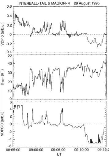
The following series of panels shows the overall view of the ‘‘multiple’’ crossing of the magnetopause which was observed by both INTERBALL satellites on 29 August 1995 between 0855 and 0915 UT. The satellites moved from the magnetosheath toward the Earth’s magnetoshpere. The INTERBALL-1 satellite was locat-ed at GSE (x, y, z) = (10, –72, –11)×103km at 0855 UT and moved nearly earthwards with the velocity of about 2.6 km/s. The MAGION–4 satellite was ahead by a distance of ~ 1020 km. This event has been examined in Nemecek et al. (1996) and it has been shown that currents of FCs can be used as a good indicator of different magnetosheath-magnetosphere regions.
The top panel in Fig. 5 shows the current of the sunward-oriented FC onboard the INTERBALL-1 satellite. As mentioned in Sect. 2.1, this current is the sum of the total ion current and the current of electrons with energy higher than 170 eV. In the left-hand part of the figure the ion current exceeds the electron one, but in
the right-hand part the FC currents become negative, thus indicating the presence of hot electrons. In accor-dance with the position of the spacecraft, the region with the high positive FC current can be considered as the magnetosheath; the hot electrons are probably of a magnetospheric origin. This classification is supported by the changes of the magnetic-field modulus, which are shown in the middle panel of Fig. 5. The magnetic field fluctuates around a value of 12 nT in the left-hand part of the figure and rises to a value of about 30 nT in the right-hand part (the highly fluctuating region in the middle of the panel will be discussed further). The measurements of the FCs onboard the MAGION–4 satellite depicted in the bottom panel demonstrate that both satellites registered the same fluctuations but at a different time. The time difference between the corre-sponding features in the top and the bottom panels is about 2 min, considerably less than the temporal distance of both satellites. It indicates that the observed structures are moving.
Figure 6 shows part of the time-interval from Fig. 5 in physical units. The plasma bulk velocity needed for the density calculation was taken from the MPS/SPS plasma spectrometer (Nemecek et al., 1997). The second panel in Fig. 6 shows the ion density measured by the INTERBALL-1 satellite. The ion density gradually decreases from 085500 to 085845 UT. This decrease can be interpreted as the encounter of the plasma depletion layer which is often observed just outside the magnetopause at these latitudes. The density falls sharply to a value less then 1/10 of the original value (at 085845 UT). Afterwards one can identify five density enhancements which are marked with numbers. The background density decreases further till 091000 UT.
The next four panels show the magnetic field mea-sured onboard the INTERBALL-1 satellite in the boundary normal (L, M, N) coordinates. The boundary normal N is taken as the minimum variance direction of the magnetic field for the period depicted in Fig. 6. The
L direction is the maximum variance direction in the
plane perpendicular to N, and M completes the right-hand set.
The structure of the low-latitude magnetopause is rather complicated and consists of a few layers which are divided by more or less distinct boundaries (Russell, 1995). We will concentrate our attention on one of them characterized by a sharp decrease of the ion density (by a factor of 5 or more) and by the increase in the magnetic field and vice versa. For briefness we will henceforth call this boundary ‘‘magnetopause’’. The first encounter of the INTERBALL-1 satellite with this boundary occurred at 085845 UT, when the ion density fell and the magnetic field increased from ~ 10 to ~ 33 nT. All five consecutive enhancements in ion density are accompanied with a decrease in the magnetic field nearly to the magnetosheath value. During the short periods of low ion density the magnetic field remains high and the fluctuation level is low. The transitions from low to high density are completed by a rotation of the magnetic field which indicates a thin current layer on this boundary. The last transition occurs at 090640 UT when the
Fig. 5. Faraday’s cup data from INTERBALL 1 (top panel ) and
MAGION-4 (bottom panel ) and magnetic-field modulus measured by the MIF-M instrument onboard the INTERBALL-1 satellite (middle panel )
magnetic field turns its direction to the magnetospheric orientation (BNand BMcomponents are negligible).
The same features can be identified in the measure-ments of the ion density onboard the MAGION-4 subsatellite shown in the top panel of Fig. 6. The time-delay between the observations made by the main satellite and the subsatellite is caused by the motion of the magnetopause. The time-delay between both satel-lites along their orbit was ~ 6 min, and the delay between the measured plasma structures is significantly lower. The different intervals of observed current variations suggest that the motion of the magnetopause is rather complicated and that the velocity of this motion is quite variable.
The major causes of the magnetopause motion – the change in the solar-wind dynamic pressure and the change in IMF direction–can be probably ruled out because, according to the measurements of the WIND at a distance of about 100 REupstream, the pressure of the
solar wind had a constant value of 2.4 nPa and the IMF was directed southward (Bzoscillated between –2.5 and
–3.5 nT ) during the time-interval 0800–0900 UT. Nevertheless, it should be taken into account that the
measurements far upstream do not always reflect the actual state of the solar wind in front of the magneto-pause (Nemecek et al., 1997).
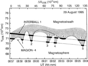
Two possible ways which the magnetopause motion can explain the observed events are illustrated in Fig. 7. The thin straight dashed lines show the position of the satellites along the YGSE axis, the bars on these lines
mark the time-intervals when the enhancements of the ion density have been registered. The number next to the particular bar relates this event to the observation depicted in Fig. 6. The solid line which connects part of the bars shows the expected position of the magneto-pause that is consistent with the model of the radial expansion of the magnetopause. This model assumes that the magnetopause is moving as a whole under the changing pressure of the solar wind and/or the changing direction and value of IMF. From this presumption we can predict that the sequence of observations of the boundary by our satellites would be as follows: the MAGION-4 – INTERBALL 1 for the outward motion and the INTERBALL-1 – MAGION-4 for the inward motion. In this case, the events at ~ 090130 and ~ 090230 UT remain unexplained and another mechanism should be involved. The thin dotted line illustrates the position of the magnetopause if the observed features are interpreted as its wavy motion.
If we follow the idea of Sibeck et al., (1990) that observed events are caused by the deformation of the magnetopause surface which moves with the velocity of the magnetosheath plasma we can estimate some dimensions of the deformation. For a tough determina-tion we can suppose that both satellites move along the
YGSE-axis (XGSE and ZGSE components are negligible)
and that the plasma moves in the –X direction. Thus we can convert the temporal scale in Fig. 7 into a spatial scale as given at the top of the figure. In this case the bottom boundary of the shadowed region represents, in some sense, the shape of the magnetopause at one arbitrary time. The magnetosheath-like plasma pulses have ~ 30-s duration, which is equal to ~ 7500 km of spatial extension along the X axis. The vertical (Y ) size
Fig. 6. Plasma and magnetic-field measurements on a pass from the
magnetosheath into the magnetosphere (from top to botom: ion density measured by the MAGION-4, ion density field provided by the INTERBALL-1, INTERBALL-1 magnetic field magnitude and three components of the magnetic field in the boundary normal coordinates.
Fig. 7. Schematic drawing of the magnetopause position
of the plasma formation should be greater than the distance between the satellites, which is ~ 1000 km. As the probability of the encounter of both satellites with the same ‘‘wave’’ is relatively high (four cases in our figure at ~ 0859, ~ 0900, ~ 0902 and ~ 0904 UT), we can assume that the amplitude of these ‘‘waves’’ is a few thousand kilometers.
4 Conclusion
We have discussed the INTERBALL observations of dense antisunward ion flows observed during the dawn magnetopause crossing on 2 August 1995. It was shown that the occurrence of these flows is correlated with the decrease in the magnetic-field intensity down to the magnetosheath value. This fact allows us to identify the boundary between the dense ion flow and less dense surrounding plasma as the magnetopause. As a result of the discussion we have presented an estimation of the shape of the magnetopause. The results of two-point observations are inconsistent with a simple model of radial expansion if a deformation of the magnetopause surface is not considered. On the other hand, all observed features can be explained by slow inward motion (comparable with the satellite velocity) of the overall magnetopause surface which is, on a small scale, modified by some process leading to the creation of the ‘‘troughs’’ in the surface. The nature of this process [pressure pulses in the magnetosheath (Sibeck et al., 1990), Kelvin-Helmholtz instability (Ogilvie and Fit-zenreiter, 1989)] can be identified only after further data processing.
As the direction and the value of the ion velocity inside the troughs are the same as in the magnetosheath the troughs should move along the magnetopause surface with the magnetosheath plasma velocity. The shape of the troughs (dotted line in Fig. 7) indicates that their velocity can be slightly lower than the magneto-sheath plasma velocity. This is a characteristic feature of the Kelvin-Helmholtz instability. A typical dimension of the troughs in the X direction is ~ 1÷2 RE, their depth
in the radial direction probably does not exceed 0.5 RE.
The observed periodicity of these events can be caused either by a boundary instability or by a pressure wave in the magnetosheath. A comparison of the discussed event with others observed by the INTERBALL satellites shows that the wavy motion is a common feature of the low-latitude dawn magnetopause.
The paper introduces first preliminary results of the magnetopause crossing study by the INTERBALL satellites, to show the possibilities of two-point obser-vations on a small scale. For a better understanding of the magnetopause motion the data should be carefully processed and supplemented with data from the other spacecraft.
Acknowledgements. The help of a number of colleagues who
contributed to the VDP proposal and to the preparation of the device is gratefully acknowledged. The last stages of the experiment preparation have been supported by the Czech Grant Agency under Contracts 205/96/1575, 202/96/0205 and 202/94/0467. The
development and construction of the MAGION–4 satellite and its scientific payload have been supported by the Czech Grant Agency under Contract 102/93/0882. Authors express their thanks to S. Romanov, N. Ryb’eva and S. Skalsky for supplying the MIF M magnetic field data.
Topical Editor, K. H. Glaßmeier thanks J. Bu¨chner and J. Sauvaud for their help in evaluating this paper.
References
Avanov, L. A., G. N. Zastenker, O. L. Vaisberg, Yu. I. Yermolaev,
Observation of small-scale solar-wind structure during the sharp increase of plasma flow velocity, Kosm. Issled., (in Russian) 22, 774, 1984.
Fairfield D. H., W. Baumjohann, G. Paschmann, H. Luehr, and D. G. Sibeck, Upstream pressure variations associated with the bow
shock and their effects on the magnetosphere, J. Geophys. Res.
95, 3773, 1990.
Gringauz K. I., G. N. Zastenker, M. Z. Khokhlov, Study of
magnetopause position variations using Faraday cups onboard Prognoz–1, 2 satellites, (in Russian), Kosm. Issled., 12, 899, 1974.
Kozak I., J. Safrankova, and Z. Nemecek, Dispersion of plasma
parameters measured by a sounding satellite during a repeated transit through a bow shock wave. Czech J. Phys., 35, 568, 1985.
Le G., C. T. Russell, and H. Kuo, Flux transfer events: Spontaneous
or driven? Geophys. Res. Lett., 20, 791, 1993.
Nemecek Z., A. Fedorov, J. Safrankova, and G. Zastenker,
Structure of the low-latitude magnetopause: MAGION–4 observation, this issue, 1996.
Nemecek Z., J. Safrankova, G. Zastenker, and P. Triska,
Multi-point study of the solar wind: INTERBALL contribution to the topic, Adv. Space Res., in print, 1997.
Ogilvie, K. W., and R. Fitzenreiter, The Kelvin-Helmholtz
insta-bility at the magnetopause and inner boundary layer surface, J.
Geophys. Res., 94, 15113, 1989.
Petrinec, S. M., and C. T. Russell, An empirical model of the size
and shape of the near-Earth magnetotail, Geophys. Res. Lett.,
20, 2695, 1993.
Roelof, L. C., and D. G. Sibeck, Magnetopause shape as a bivariate
function of interplanetary magnetic field Bz and solar wind
dynamic pressure, J. Geophys. Res., 98, 21421, 1993.
Russell, C. T., The structure of the magnetopause, in Physics of the
Magnetopause Eds. P. Song et al., Geophysical Monograph 90,
AGU, 81, 1995.
Russell, C. T., and R. C. Elphic, Initial ISEE magnetometer results:
Magnetopause observations, Space Sci Rev., 22, 681, 1978.
Safrankova, J., G. Zastenker, A. Fedorov, Z. Nemecek, M. Simer-sky. L. Prech, O. Vaisberg. Yu. Sharko, T. Romasenko, A. Leibov, M. Richter, T. Lesina, N. Plusnina, and N. Yanovskaja,
Omnidirectional plasma sensor VDP, in INTERBALL Mission
and Payload, Eds. Yu. Galperin et al., CNES-IKI-RSA, 195,
1995.
Sibeck, D. G., The magnetospheric response to foreshock pressure
pulses, in Physics of the Magnetopause, Geophys. Monograph 90, 293, 1995.
Sibeck, D. G., W. Baumjohann, R. C. Elphic, D. H. Fairfield, J. T. Fennell, W. B. Gail, L. J. Lanzerotti, R. E. Lopez, H. Luehr, A. T. Y. Lui, C. G. Maclennan R. W. McEntire, T. A. Potemra, T. J. Rosenberg, and K. Takalzashi, The magnetospheric
response to 8-min-period strong-amplitude upstream pressure variations, J. Geophys. Res., 94, 2505, 1989a.
Sibeck, D. G., W. Baumjohann, and R. E. Lopez, Solar wind
dynamic pressure variations and transient magnetospheric signatures. Geophys. Res. Lett., 16, 13, 1989b.
Sibeck, D. G., R. P. Lepping, and A. J. Lazarus, Magnetic field line
draping in the plasma depletion layer, J. Geophys. Res., 95, 2433, 1990.
Vaisberg O. L., Gorn L. S., Yermolaev Yu., Zastenker G. N., Zakharov D. S., Zertsalov A. A., Klimashov A. A., Lein E. L. Leibov A. V. Omelchenko A. N., Pomogaev V. V, Romanov S. A., Smirnov V. N., Stefanovich A. E., Tyomniy V. V., Khazanov B. I., Shifrin A. V., Experiment on interplanetary and
magnetosphere plasma diagnostics onboard Venera-11, 12 spacecraft and Prognoz-7 satellite, (in Russian) Kosm. Issled.
17, 780, 1979.
Zastenker G. N., Yermolaev Yu. I., Pinter S., Nemecek Z., Safrankova J., Belikova A. B., Leibov A. V., Prokhorenko V. I, Stefanovich A. V., Bedrikov A. G., Karimov B. T., Solar wind
observations with high time resolution Kosm. ssled. (in Russian)
20, 900 1982.