Quantification of Lambda (Λ) in multi-elemental compound-specific isotope analysis

HAL Id: hal-03082804

https://hal-amu.archives-ouvertes.fr/hal-03082804

HAL is a multi-disciplinary open access archive for the deposit and dissemination of sci-entific research documents, whether they are pub-lished or not. The documents may come from teaching and research institutions in France or abroad, or from public or private research centers.

L’archive ouverte pluridisciplinaire HAL, est destinée au dépôt et à la diffusion de documents scientifiques de niveau recherche, publiés ou non, émanant des établissements d’enseignement et de recherche français ou étrangers, des laboratoires publics ou privés.

Quantification of Lambda (Λ) in multi-elemental

compound-specific isotope analysis

Patrick Höhener, Gwenael Imfeld

To cite this version:

Patrick Höhener, Gwenael Imfeld. Quantification of Lambda (Λ) in multi-elemental compound-specific isotope analysis. Chemosphere, Elsevier, 2021, 267, pp.129232. �10.1016/j.chemosphere.2020.129232�. �hal-03082804�

Quantification of Lambda () in multi-elemental

compound-1

specific isotope analysis

2

1_{Patrick Höhener}* _and 2_{Gwenaël Imfeld}

3

1_{Aix Marseille University – CNRS, UMR 7376, Laboratory of Environmental Chemistry,} 4

Marseille, France, Phone No. 0033413551034 5

*Corresponding author. patrick.hohener@univ-amu.fr 6

2 _{Laboratory of Hydrology and Geochemistry of Strasbourg (LHyGeS), Université de} 7

Strasbourg, UMR 7517 CNRS/EOST, 1 Rue Blessig, 67084, Strasbourg Cedex, France 8

Short communication to Chemosphere, https://doi.org/10.1016/j.chemosphere.2020.129232

9

10

Highlights

11

The parameter  represents dual element stable isotope data 12

Two conventions for quantifying  give different  values 13

Linear regressions of delta values in a dual element plot overestimate  14

We show that only the ln-transformed isotope ratios should be fitted 15 16 17 0 20 40 60 80 0 1 2 3 4 5 Dd 2 H (‰ ) Dd13_{C (‰)}

 ?

Short Communication Chemosphere 2

ABSTRACT

18

In multi-elemental compound-specific isotope analysis the lambda () value expresses the 19

isotope shift of one element versus the isotope shift of a second element. In dual-isotope plots, 20

the slope of the regression lines typical reveals the footprint of the underlying isotope effects 21

allowing to distinguish degradation pathways of an organic contaminant molecule in the 22

environment. While different conventions and fitting procedures are used in the literature to 23

determine , it remains unclear how they affect the magnitude of  Here we generate synthetic 24

data for benzene d2H and d13C with two enrichment factors H and C using the Rayleigh equation 25

to examine how different conventions and linear fitting procedures yield distinct . Fitting an 26

error-free data set in a graph plotting the d2H versus d13C overestimates  by 0.225%∙ 𝜀𝐻/𝜀𝐶, 27

meaning that if 𝜀𝐻/𝜀𝐶is larger than 22,  is overestimated by more than 5%. The correct fitting 28

of  requires a natural logarithmic transformation of d2_{H versus d}13_{C data. Using this} 29

transformation, the ordinary linear regression (OLR), the reduced major-axis (RMA) and the 30

York methods find the correct , even for large 𝜀𝐻/𝜀𝐶. Fitting a dataset with synthetic data with 31

typical random errors let to the same conclusion and positioned the suitability of each regression 32

method. We conclude that fitting of non-transformed d values should be discontinued. The 33

validity of most previous  values is not compromised, although previously obtained  values 34

for large 𝜀𝐻/𝜀𝐶 could be corrected using our error estimation to improve comparison. 35

Key Words

36

Stable isotopes, pollution, assessment, bioremediation 37

1. Introduction

38

Multi-elemental Compound-Specific Isotope Analysis (ME-CSIA) is increasingly used to assess 39

the fate of pollutants such as hydrocarbons (Vogt et al., 2016), chlorinated solvents solvents 40

(Palau et al., 2014, Audi-Miro et al., 2015, Palau et al., 2016), nitrates (Xue et al., 2009), 41

perchlorates (Sturchio et al., 2012) and pesticides (Ponsin et al., 2019, Melsbach et al., 2020) in 42

the environment. The slope of the dual-isotope plot (Lambda, ) reflects changes of the isotope 43

ratios of each element, which can be specific to a reaction mechanism, and thus inform about 44

transformation processes in the laboratory or in the field. (Vogt et al., 2016, Elsner, 2010) 45

Several studies (Masbou et al., 2018, Huntscha et al., 2014, Lian et al., 2019, Bouchard et al., 46

2018, Vogt et al., 2016, Elsner, 2010, Ojeda et al., 2019) refer to  using the simple definition in 47

eq. 1, which is written here as an example for hydrogen vs carbon dvalues (eq. 1). 48 𝛬= ∆𝛿 𝐻 2 ∆𝛿 𝐶 13 ≈ 𝜀𝐻 𝜀𝐶 eq. 1 49

where Dd is the change of isotope ratios from initial values, and  are the enrichment factors for 50

hydrogen and carbon. The Lambda () is an important parameter in ME-CSIA. It is a practical 51

and unitless number which characterizes a specific process. It can be determined either by simply 52

using the two enrichment factors and the right-hand side of equation 1 on one hand, or from 53

regression analysis in a dual-isotope plots with isotope data of one element versus data of 54

another element in the same compound (Figure 1). Lambda values were obtained in many studies 55

(Ojeda et al., 2019, Palau et al., 2017, Rosell et al., 2007, Rodriguez-Fernandez et al., 2018, 56

Rodriguez-Fernandez et al., 2018, Dogan-Subasi et al., 2017, Cretnik et al., 2013, Audi-Miro et 57

al., 2013, Palau et al., 2014, Lian et al., 2019, Badin et al., 2016, Mogusu et al., 2015, Ponsin et 58

Short Communication Chemosphere 4

al., 2019, McKelvie et al., 2009, Pati et al., 2012) from the regression analyses in dual-isotope 59

plots (i.e., ratios of one isotope as a function of another isotope as delta values; Figure 1A). 60

Another mathematical notation for  has been described in detail in (Wijker et al., 2013) (eq. 2), 61

noted here for hydrogen and carbon isotopes: 62 𝛬= 𝑙𝑛[(𝛿 𝐻/1000 2 _{+1)/(𝛿 𝐻} 0/1000 2 _+1)] 𝑙𝑛[(𝛿 𝐶/1000 13 +1)/(𝛿 𝐶13 0/1000 +1)] ≈𝜀𝐻 𝜀𝐶 eq. 2 63

Figure 1B shows an example of a dual-isotope plot to determine  using eq. 2, named below the 64

ln-transformed d data. This way of obtaining  was used e.g. in ( Schilling et al., 2019 a+b). 65

Apart from those two different conventions for plotting isotope data, different methods of linear 66

regression were proposed to obtain . These include the ordinary linear regression (OLR), the 67

reduced major axis regression (RMA), and the York linear regression, which have been 68

compared recently (Ojeda et al., 2019). 69

The objective of this short comment is to compare the two conventions (i.e., A, with eq. 1 and B, 70

with 2) to determine  values and the associated uncertainty from a dual-isotope plot. Two 71

synthetic datasets were generated, one without random error, and a second one with random 72

errors mimicking measurement uncertainties. Each dataset was fitted with the ordinary linear 73

regression (OLR), the reduced major-axis (RMA) and the York regression methods and results 74

were compared. 75

2. Methods

76

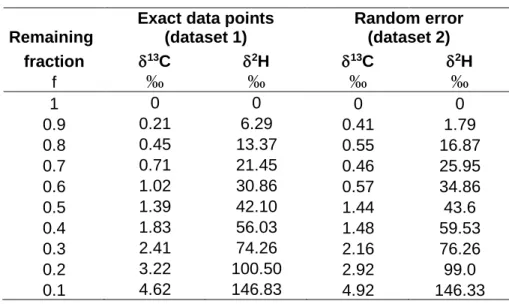
The Rayleigh equation (eq. 3) (Aelion et al., 2010) was used to generate 10 synthetic exact data 77

points for each element (i.e., C and H). We used isotope enrichment factors for carbon and 78

hydrogen corresponding to methanogenic degradation of benzene: C = -2.0 and H = -59.5 ‰. 79

(Mancini et al., 2003) The remaining fraction (𝑓) of benzene was varied from 1 to 0.1 in steps of 80

0.1 (see data set in the supplementary data). 81

𝑅 𝑅0 = 𝑓

(𝛼−1) _{eq. 3}

82

Where R is the isotope ratio, R0 is the initial isotope ratio (chosen as the R of international

83

standard Rstd), 𝑓 is the fraction of compound remaining (C/C0), and  is the isotope fractionation 84

factor (equal to /1000 +1). The resulting isotope ratios were expressed as d values [d =(R/Rstd -85

1)*1000; Rstd,H=1.5575E-4; Rstd,C=0.011237] and plotted in Figure 1A (Dd vs DdC, eq .1) 86

and 1B (ln-transformed data, eq. 2). The resulting slopes should reflect the ratio of original 87

isotopic enrichment values, -59.50/-2.00, thus =29.75. 88

A second dataset was generated using the same enrichment factors but introducing random errors 89

in the calculated d values (see Table S1 in supplementary data). The d values of this set had a 90

random error of up to ± 0.5 ‰ for carbon and up to ± 5.0 ‰ for hydrogen, which corresponds to 91

the typical total analytical uncertainties. 92

Finally, 25 more datasets (data not shown) were generated in the same manner as dataset 1 93

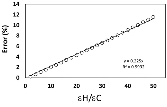
without random error, keeping C = -2.0 ‰ and varying H over H / C ratios from 2 to 50. Each 94

of these data sets was fitted with OLR, and the overestimation of fit A over fit B was quantified 95

and plotted in Figure 2 as a function of 𝜀𝐻/𝜀𝐶 96

The datasets were generated with Excel (Microsoft), Vs. 2011), and linear regressions (OLR, 97

RMA and York) were calculated with a script adapted from Ojeda et al. (2019) and were not 98

forced through the origin. 99

Short Communication Chemosphere 6

3. Results

100

The dataset 1 with the raw Dd values (eq. 1) does not plot on a perfect straight line (Figure 1A). 101

The slope becomes steeper with increasing d values (smaller 𝑓). An OLR gives a mean  of 102

31.70 ± 0.21 (R2 >0.99), which overestimates the true  of 29.75 by 6.6 %. In contrast, the 103

dataset 1 with ln-transformed d values (eq. 2) plots perfectly on a straight line with a slope of 104

29.74 ± 0.02 with an R2 of 1.0000 (Figure 1B), which matches the true . 105 106 107 108 109 110 111 112 113 114

Fig. 1. Dual-isotope plot of A) raw Dd values (according to eq. 1), and B) ln-transformed d

115

values (according to eq. 2). Crosses correspond to exact datapoints (dataset 1) and grey

116

diamonds are datapoints with random error (dataset 2).

117

Dd

vs

Dd

plot

A:

Dd

H (

‰

)

Dd

C (‰)

ln((d

C/1000+1)/(d

C

/1000+1))

ln(

(d

H/1

00

0+

1)

/(

d

H

/1

00

0+

1))

B: ln transformed plot

118

Table 1: Comparison of  calculated with the raw Dd values (convention A, eq. 1) and the ln-transformed d values (convention B, eq.

119

2) using the OLR, RMA and York methods, for the exact data points (dataset 1) and data generated with a random error (dataset 2).

120

121

Exact data points (dataset 1)

Dd vs Dd ln-transformed

 SE R2  _{SE R}2

OLR 31.70 0.21 >0.99 29.74 0.02 1.00

RMA 31.71 0.19 >0.99 29.74 0.02 1.00

York 31.71 3.77 >0.99 29.74 3.56 1.00

SE: Standard error of 

122 123 124 125 126 127

Random error (dataset 2)

Dd vs Dd ln-transformed  SE R2  _{SE R}2 30.08 2.13 0.96 28.15 2.16 0.95 30.67 1.90 0.98 28.80 1.93 0.98 31.17 3.68 0.96 29.33 3.50 0.95 128

Short Comm. Chemosphere 8

The overestimation of  calculated with convention A compared to convention B was quantified 129

as a function of H/C ranging from 2 to 50 (Fig. 2; OLR method)). 130

131

Fig. 2 Overestimation of  () as a function of H/C (symbols) when convention A (eq. 1) is 132

used. The straight dotted line is the mean error increase of 0.225% per H/C.

133

Figure 2 shows that the error in a graph plotting the d values like in Fig. 1.A overestimates  by 134

11.5 % when H / C reaches 50. The increase of the error is almost linear with a slope of 0.225% 135

per H / C  136

4. Discussion

137

The use of the exact (error-free) synthetic dataset to compare conventions A (eq. 1) and B (eq. 2) 138

emphasized that  calculated with convention A is linearly overestimated (eq.1). The difference 139 y = 0.225x R² = 0.9992

0

2

4

6

8

10

12

14

0

10

20

30

40

50

H/C

Err

or

(%)

of  obtained with convention A and B has a pure mathematical cause (Wijker et al., 2013): 140

equation 1 is derived from eq. 2 by a Taylor series expansion which is only approximate. 141

Höhener and Atteia (Höhener and Atteia, 2014) derived mathematically the dependence of the 142

slope  on the remaining, non-degraded fraction f in a dual-isotope plot (eq. 4) based on the 143

theory of Rayleigh distillation. 144 𝛬 = ∆𝛿 𝐻 2 ∆𝛿 𝐶 13 = 𝑓 1000𝜀𝐻−1 𝑓 1000𝜀𝐶−1 eq. 4 145

Equation 4 (eq. 16 in (Höhener and Atteia, 2014)) shows that  is increasing with decreasing f , 146

as observed in Figure 1A. Thus, for f close to one,  is 29.75, while for f = 0.1,  is 31.80. 147

All three regression methods tested for convention A with dataset 1 gave a similar  of 31.7, 148

although their standard errors (SE) differed (Table 1). OLR and RMA methods gave a narrow SE 149

(0.21 and 0.19, respectively), leading us to the wrong conclusion that  is > 31. Regression with 150

the York method gave a larger SE ( = 31.71 ± 3.68, Tab. 1), which represents a correct but 151

inaccurate description of the true  of 29.75. For convention B and dataset 1, all three regression 152

methods find the true , although only the OLR and RMA method yielded accurate  within 153

narrow error limits. 154

Measured isotope ratios are always affected by random errors from measurements, which were 155

accounted for in dataset 2 to calculate  (Table 1). All three methods predicted    using 156

convention A, and  was associated with large SE, ranging from 1.90 to 3.68. Using convention 157

B,  ranged from 28.15 to 29.33, with SE ranging from 1.9 (RMA) to 3.5 (York). For dataset 2, 158

RMA was the best fitting method, yielding the narrower SE, while both OLR and York gave 159

Short Comm. Chemosphere 10

accurate predictions also with higher error. All regressions match thus the true value of 29.75 160

within their error limits. 161

To sum up, the error-free data in a dual-isotope plot with Dd vs Dd values do not lie on a straight 162

line and thus should not be fitted with any linear regression. The slope in a Dd vs Dd plot is per 163

definition a function of the progress of reaction f (eq. 4). A non-linear curve is obtained, 164

especially when the orders of magnitude of the enrichment factors differ. Linear regressions in 165

such plots yield  that overestimate the true  and should be discontinued. The correct 166

convention to linearize data is provided in eq. 2 and should be applied as in Figure 1B to obtain 167

accurate  OLR and RMA regression methods yield narrower error estimates, whereas the York 168

method finds the true  within a larger error margin. The validity of most previously obtained  169

values with convention A might not be compromised given the total uncertainty of the 170

experimental and analytical methods. However, in a few cases with large 𝜀𝐻/𝜀𝐶 ratios, corrections 171

might be applied in order to compare optimally all  values. The simple procedure to follow 172

consists in using Fig. 2 of our manuscript, selecting the appropriate ratio of epsilons, reporting 173

the corresponding error percentage (which is the percentage of overestimation) to lower  by this 174

percentage. Worthy of note, if experimental data still plotting nonlinearly on a ln-transformed 175

plot with eq. 2, as e.g. in (Dorer et al., 2014), another process may be involved, including a very 176

strong hydrogen fractionation (tunneling), concentration-dependent fractionation and/or 177

instrumental non-linearity. In these specific cases,  cannot be expressed as a constant number. 178

Acknowledgments

This work is funded by the French National research Agency ANR through grant ANR-18-CE04-180

0004-01, project DECISIVE. 181

Supplementary data

Table of synthetic datasets used in this work. 183

184

185

5. References

186

Aelion, C. M., Höhener, P., Hunkeler, D., Aravena, R. Environmental Isotopes in Biodegradation 187

and Bioremediation. CRC Press (Taylor and Francis), Boca Raton, 2010. 188

Audi-Miro, C., Cretnik, S., Otero, N., Palau, J., Shouakar-Stash, O., Soler, A., Elsner, M., 2013. 189

Cl and C isotope analysis to assess the effectiveness of chlorinated ethene degradation by 190

zero-valent iron: Evidence from dual element and product isotope values. Appl. Geochem. 191

32, 175-183. 192

Audi-Miro, C., Cretnik, S., Torrento, C., Rosell, M., Shouakar-Stash, O., Otero, N., Palau, J., 193

Elsner, M., Soler, A., 2015. C, Cl and H compound-specific isotope analysis to assess 194

natural versus Fe(0) barrier-induced degradation of chlorinated ethenes at a contaminated 195

site. J. Hazard. Mat. 299, 747-754. 196

Badin, A., Broholm, M. M., Jacobsen, C. S., Palau, J., Dennis, P., Hunkeler, D., 2016. 197

Identification of abiotic and biotic reductive dechlorination in a chlorinated ethene plume 198

after thermal source remediation by means of isotopic and molecular biology tools. J. 199

Contam. Hydrol. 192, 1-19. 200

Short Comm. Chemosphere 12

Bouchard, D., Hunkeler, D., Madsen, E., Buscheck, T., Daniels, E., Kolhatkar, R., DeRito, C., 201

Aravena, R., Thomson, N., 2018. Application of Diagnostic Tools to Evaluate Remediation 202

Performance at Petroleum Hydrocarbon-Impacted Sites. Ground Wat. Monitor. Remed. 38, 203

88-98. 204

Cretnik, S., Thoreson, K. A., Bernstein, A., Ebert, K., Buchner, D., Laskov, C., Haderlein, S., 205

Shouakar-Stash, O., Kliegman, S., McNeill, K., Elsner, M., 2013. Reductive Dechlorination 206

of TCE by Chemical Model Systems in Comparison to Dehalogenating Bacteria: Insights 207

from Dual Element Isotope Analysis (C-13/C-12, Cl-37/Cl-35). Environ. Sci. Technol. 47, 208

6855-6863. 209

Dogan-Subasi, E., Elsner, M., Qiu, S., Cretnik, S., Atashgahi, S., Shouakar-Stash, O., Boon, N., 210

Dejonghe, W., Bastiaens, L., 2017. Contrasting dual (C, Cl) isotope fractionation offers 211

potential to distinguish reductive chloroethene transformation from breakdown by 212

permanganate. Sci. Tot. Environ. 596, 169-177. 213

Dorer, C., Höhener, P., Hedwig, N., Richnow, H. H., Vogt, C., 2014. Rayleigh-based concept to 214

tackle strong hydrogen fractionation in dual-isotope-analysis - the example of ethylbenzene 215

degradation of Aromatoleum aromaticum. Environ. Sci. Technol. 48, 5788-–5797. 216

Elsner, M., 2010. Stable isotope fractionation to investigate natural transformation mechanisms 217

of organic contaminants: principles, prospects and limitations. J. Environ. Monitoring 12, 218

2005-2031. 219

Huntscha, S., Hofstetter, T., Schymanski, E., Spahr, S., Hollender, J., 2014. Biotransformation of 220

Benzotriazoles: Insights from Transformation Product Identification and Compound-221

Specific Isotope Analysis. Environ. Sci. Technol. 48, 4435-4443. 222

Höhener, P., Atteia, O., 2014. Rayleigh equation for evolution of stable isotope ratios in 223

contaminant decay chains. Geochim. Cosmochim. Acta 126, 70-77. 224

Lian, S., Wu, L., Nikolausz, M., Lechtenfeld, O., Richnow, H., 2019. H-2 and C-13 isotope 225

fractionation analysis of organophosphorus compounds for characterizing transformation 226

reactions in biogas slurry: Potential for anaerobic treatment of contaminated biomass. 227

Water Res. 163, 114882. 228

Mancini, S. A., Ulrich, A. C., Lacrampe-Couloume, G., Sleep, B., Edwards, E. A., Sherwood-229

Lollar, B., 2003. Carbon and Hydrogen Isotopic Fractionation during Anaerobic 230

Biodegradation of Benzene. Appl. Environ. Microbiol. 69, 191-198. 231

Masbou, J., Drouin, G., Payraudeau, S., Imfeld, G., 2018. Carbon and nitrogen stable isotope 232

fractionation during abiotic hydrolysis of pesticides. Chemosphere 213, 368-376. 233

McKelvie, J., Hyman, M., Elsner, M., Smith, C., Aslett, D., Lacrampe-Couloume, G., Sherwood 234

Lollar, B., 2009. Isotopic Fractionation of Methyl tert-Butyl Ether Suggests Different Initial 235

Reaction Mechanisms during Aerobic Biodegradation. Environ. Sci. Technol. 43, 2793-236

2799. 237

Melsbach, A., Torrento, C., Ponsin, V., Bolotin, J., Lachat, L., Prasuhn, V., Hofstetter, T., 238

Hunkeler, D., Elsner, M., 2020. Dual-Element Isotope Analysis of Desphenylchloridazon to 239

Investigate Its Environmental Fate in a Systematic Field Study: A Long-Term Lysimeter 240

Experiment. Environ. Sci. Technol. 54, 3929-3939. 241

Mogusu, E., Wolbert, J., Kujawinski, D., Jochmann, M., Elsner, M., 2015. Dual element (N-242

15/N-14, C-13/C-12) isotope analysis of glyphosate and AMPA by derivatization-gas 243

Short Comm. Chemosphere 14

chromatography isotope ratio mass spectrometry (GC/IRMS) combined with LC/IRMS. 244

Anal. Bioanal. Chem. 407, 5249-5260. 245

Ojeda, A., Phillips, E., Mancini, S., Sherwood Lollar, B., 2019. Sources of Uncertainty in 246

Biotransformation Mechanistic Interpretations and Remediation Studies using CSIA. Anal. 247

Chem. 91, 9147-9153. 248

Palau, J., Jamin, P., Badin, A., Vanhecke, N., Haerens, B., Brouyere, S., Hunkeler, D., 2016. Use 249

of dual carbon-chlorine isotope analysis to assess the degradation pathways of 1,1,1-250

trichloroethane in groundwater. Water Res. 92, 235-243. 251

Palau, J., Shouakar-Stash, O., Hunkeler, D., 2014. Carbon and Chlorine Isotope Analysis to 252

Identify Abiotic Degradation Pathways of 1,1,1-Trichloroethane. Environ. Sci. Technol. 48, 253

14400-14408. 254

Palau, J., Yu, R., Mortan, S., Shouakar-Stash, O., Rosell, M., Freedman, D., Sbarbati, C., 255

Fiorenza, S., Aravena, R., Marco-Urrea, E., Elsner, M., Soler, A., Hunkeler, D., 2017. 256

Distinct Dual C-C1 Isotope Fractionation Patterns during Anaerobic Biodegradation of 1,2-257

Dichloroethane: Potential To Characterize Microbial Degradation in the Field. Environ. 258

Sci. Technol. 51, 2685-2694. 259

Pati, S., Shin, K., Skarpeli-Liati, M., Bolotin, J., Eustis, S., Spain, J., Hofstetter, T., 2012. Carbon 260

and Nitrogen Isotope Effects Associated with the Dioxygenation of Aniline and 261

Diphenylamine. Environ. Sci. Technol. 46, 11844-11853. 262

Ponsin, V., Torrento, C., Lihl, C., Elsner, M., Hunkeler, D., 2019. Compound-Specific Chlorine 263

Isotope Analysis of the Herbicides Atrazine, Acetochlor, and Metolachlor. Anal. Chem. 91, 264

14290-14298. 265

Rodriguez-Fernandez, D., Heckel, B., Torrento, C., Meyer, A., Elsner, M., Hunkeler, D., Soler, 266

A., Rosell, M., Domenech, C., 2018. Dual element (C-Cl) isotope approach to distinguish 267

abiotic reactions of chlorinated methanes by Fe(0) and by Fe(II) on iron minerals at neutral 268

and alkaline pH. Chemosphere 206, 447-456. 269

Rosell, M., Barcelo, D., Rohwerder, T., Breuer, U., Gehre, M., Richnow, H. H., 2007. Variations 270

in C-13/C-12 and D/H enrichment factors of aerobic bacterial fuel oxygenate degradation. 271

Environ. Sci. Technol. 41, 2036-2043. 272

Schilling, I., Bopp, C., Lal, R., Kohler, H., Hofstetter, T., 2019a. Assessing Aerobic 273

Biotransformation of Hexachlorocyclohexane Isomers by Compound-Specific Isotope 274

Analysis. Environ. Sci. Technol. 53, 7419-7431. 275

Schilling, I., Hess, R., Bolotin, J., Lal, R., Hofstetter, T., Kohler, H., 2019b. Kinetic Isotope 276

Effects of the Enzymatic Transformation of gamma-Hexachlorocyclohexane by the 277

Lindane Dehydrochlorinase Variants LinA1 and LinA2. Environ. Sci. Technol. 53, 2353-278

2363. 279

Sturchio, N. C., Hoaglund, J. R., Marroquin, R. J., Beloso, A. D., Heraty, L. J., Bortz, S. E., 280

Patterson, T. L., 2012. Isotopic mapping of groundwater perchlorate plumes. Ground Water 281

50, 94-102. 282

Short Comm. Chemosphere 16

Vogt, C., Dorer, C., Musat, F., Richnow, H. H., 2016. Multi-element isotope fractionation 283

concepts to characterize the biodegradation of hydrocarbons from enzymes to the 284

environment. Curr. Opin. Biotechnol. 41, 90-98. 285

Wijker, R., Adamczyk, P., Bolotin, J., Paneth, P., Hofstetter, T., 2013. Isotopic Analysis of 286

Oxidative Pollutant Degradation Pathways Exhibiting Large H Isotope Fractionation. 287

Environ. Sci. Technol. 47, 13459-13468. 288

Xue, D., Botte, J., De Baets, B., Accoe, F., Nestler, A., Taylor, P., Van Cleemput, O., Berglund, 289

M., Boeckx, P., 2009. Present limitations and future prospects of stable isotope methods for 290

nitrate source identification in surface- and groundwater. Water Res. 43, 1159-1170. 291 292 293 294 295 296 297 298 299 300 301

302

SUPPLEMENTARY DATA

303

Quantification of Lambda () in multi-elemental compound-specific isotope

analysis

1_{Patrick Höhener}* _and 2_{Gwenaël Imfeld}

306

1_{Aix Marseille University – CNRS, UMR 7376, Laboratory of Environmental Chemistry, Marseille,}

307

France 308

*Corresponding author. patrick.hohener@univ-amu.fr 309

2 _{Laboratory of Hydrology and Geochemistry of Strasbourg (LHyGeS), Université de Strasbourg, UMR} 310

7517 CNRS/EOST, 1 Rue Blessig, 67084, Strasbourg Cedex, France 311

Contents:

Table S1: Datasets used in this work

Table S1: Synthetic data shown in Figure 1 and used for fitting.

314

Remaining

Exact data points (dataset 1) Random error (dataset 2) fraction d13_C d2_H d13_C d2_H f ‰ ‰ ‰ ‰ 1 0 0 0 0 0.9 0.21 6.29 0.41 1.79 0.8 0.45 13.37 0.55 16.87 0.7 0.71 21.45 0.46 25.95 0.6 1.02 30.86 0.57 34.86 0.5 1.39 42.10 1.44 43.6 0.4 1.83 56.03 1.48 59.53 0.3 2.41 74.26 2.16 76.26 0.2 3.22 100.50 2.92 99.0 0.1 4.62 146.83 4.92 146.33 315

Short Comm. Chemosphere 18

316