Monitoring Suspended Particle Matter Using GOCI Satellite Data After the Tohoku (Japan) Tsunami in 201

HAL Id: hal-02894360

https://hal.archives-ouvertes.fr/hal-02894360

Submitted on 8 Jul 2020

HAL is a multi-disciplinary open access

archive for the deposit and dissemination of

sci-entific research documents, whether they are

pub-lished or not. The documents may come from

teaching and research institutions in France or

abroad, or from public or private research centers.

L’archive ouverte pluridisciplinaire HAL, est

destinée au dépôt et à la diffusion de documents

scientifiques de niveau recherche, publiés ou non,

émanant des établissements d’enseignement et de

recherche français ou étrangers, des laboratoires

publics ou privés.

Satellite Data After the Tohoku (Japan) Tsunami in 201

Audrey Minghelli, Manchun Lei, Sabine Charmasson, Vincent Rey, Malik

Chami

To cite this version:

Audrey Minghelli, Manchun Lei, Sabine Charmasson, Vincent Rey, Malik Chami. Monitoring

Sus-pended Particle Matter Using GOCI Satellite Data After the Tohoku (Japan) Tsunami in 201. IEEE

Journal of Selected Topics in Applied Earth Observations and Remote Sensing, IEEE, 2019, 12 (2),

pp.567-576. �10.1109/JSTARS.2019.289406�. �hal-02894360�

Monitoring Suspended Particle Matter using

GOCI satellite data after the Tohoku (Japan)

tsunami in 2011

Audrey MINGHELLI, Université de Toulon, CNRS, LIS UMR 7296, 83957 La Garde, France

Manchun LEI, Université Paris-Est, LaSTIG, IGN, ENSG, 94160 Saint-Mandé, France

Sabine CHARMASSON, Institut de radioprotection et de Sûreté Nucléaire PSE-

ENV/SRTE/LRTA, Centre Ifremer, 83500, La Seyne sur Mer, France

Vincent REY, Aix Marseille Université, CNRS/INSU, IRD, Mediterranean Institute of

Oceanography (MIO), UM110, 13288 Marseille, France

Malik CHAMI, Sorbonne Université, CNRS-INSU, LATMOS, Boulevard de l’Observatoire, CS 34229,

06304 Nice Cedex, France

and Institut Universitaire de France, 75231 Paris, France

Abstract— The Fukushima Daiichi nuclear disaster that

occurred on March 11, 2011 was caused by the Tohoku tsunami which was itself triggered by the devastating 9.0Mw moment magnitude earthquake. The present study investigates spatial and temporal changes of Suspended Particulate Matter (SPM) content in the North-Eastern part of Japan (Pacific Ocean) using a geostationary ocean color sensor. The Geostationary Ocean Color Imager (GOCI), which is centered on the Korean peninsula but could also observe the Japanese area, is able to acquire 8 images per day, thus allowing the analysis of rapid daily changes in water mass. The analysis of GOCI data shows that SPM concentration notably increased both along the coast and within the Bay of Sendai shortly after the tsunami. Motionless patterns of SPM were observed at 2, 14, 25 and 37 km from the coast. It is shown that

SPM concentration rapidly decreased one month later. The SPM

concentration did not remain high the following year, contrary to what was observed for the Sumatra Tsunami in 2004. The origin of SPM is also investigated in this study. Our analysis suggests that some of the SPM originates from the resuspension of bottom sediments due to the reflection of the tsunami on the coastline that leads to the migration of marine particles towards the sea surface. The fate of the SPM concentration is then discussed based on the analysis of meteorological conditions, river discharge and tsunami wave properties.

Index Terms— Ocean color, GOCI, Suspended Particulate

Matter, Tohoku tsunami.

I. Introduction

T

heoccurred at 14:46 JST (05:46 UTC) on March 11, 2011, had megathrust earthquake off the coast of Japan that an epicenter approximately 72 km East of the Oshika Peninsula of Tohoku and a hypocenter in the Pacific Ocean at a depth of

approximately 32 km [1]. It was the most powerful earthquake ever recorded in Japan. Many coastal tide gauges on the Pacific coast stopped recording after the first phase of the tsunami, which shows an amplitude greater than 9 m. This is because of power failure or because the stations were washed away by the tsunami. However, three offshore gauges, one GPS wave gauge (Iwate S at ~200 m water depth) and two cabled pressure- gauges (TM-2 at ~1,000 m and TM-1 at 1,600 m depth), were able to record the two stages of the tsunami: The water level gradually rose to 2 m during the first 10 minutes, then an impulsive tsunami wave with 3-5 m amplitude having a shorter period (~8 min) was recorded. At southern GPS (Fukushima) and coastal (Onahama) gauges, two similar pulses were recorded, and their periods were respectively 11 and 15 min [2]. The tsunami waves, which reached heights of up to 15 meters in the Fukushima Prefecture and in the Sendai area, traveled up to 10 km inland [1].

Such a massive tsunami led to a loss of electrical power that triggered a cooling system failure at the Fukushima Daiichi Nuclear Power Plants (FDNPP) where at least three nuclear reactors suffered explosions. Radioactive releases in the environment occurred from deliberate venting to reduce gas pressure in the containment structures and deliberate discharge of coolant water into the sea. However, the main radioactive releases came from explosive releases into the atmosphere, thus leading to significant fallout on both land and ocean. Other direct discharges to the ocean were caused by water leakage from the reactor buildings occurred [3].

Estimates of radioactive releases into the ocean tend to converge between 15 and 20 PBq for the combined FDNPP inputs of 137Cs from atmospheric fallout (peaking March 15)

and direct discharge (peaking April 6) in the North Pacific [4], [3].

Fortunately, the oceanic currents existing off the Fukushima coast, which are among the strongest currents in the world [5], transported most of the contaminated waters far out into the Pacific Ocean, thus inducing a massive dispersion of the radioactive elements [6]. However, long-term sources along the coast in the vicinity of the nuclear plant are still conveying radioactive elements from land to ocean through river flows, rivers, runoff and contaminated underground water [3], [7].

Since various radionuclides are known to be particle reactive [3], it could be relevant to assess the impact of the tsunami on

SPM concentrations off the coast of Fukushima using remote

sensing data. It was previously shown that an increase in SPM concentration was observed at different places in the Indian Ocean after the tsunami of Sumatra which occurred in 2004 [8]. Such a SPM variation was monitored for one year (2005) by satellite image analysis throughout the northeastern part of the Indian Ocean [9], [10]. By analyzing IRS-P4 OCM satellite data, Singh et al. [11] reported that the SPM and chlorophyll concentration increased after earthquakes as a result of the intense shaking due to intense seismic activity along the west coast of India in 2001. Previous studies also reported that SPM and chlorophyll concentrations were modified along the east coast of the USA and east coast of India after the passage of cyclones [8], [12]-[18].

The turbidity current generated by the Tohoku tsunami and the subsequent offshore deposits have been well documented [19], [20], whereas information about offshore tsunami deposits is relatively poorly documented. Sedimentation and erosion in inner bay and open ocean locations have been estimated to reach up to several meters, suggesting that the tsunami’s shear force was strong near the coast. On the other hand, sandy and muddy deposits a few centimeters thick were observed at about 100 m and 6000 m depth. Goto et al. [21] suggested that the tsunami likely gave rise to a resuspension of sea bottom sediments and that suspended material flowed downslope as a turbidity current or suspended flow.

Satellite images can provide information concerning the water turbidity. However, they have not yet been used, to our knowledge, in monitoring the SPM of Fukushima after the tsunami. This lack of research is probably due to the high cloud coverage over the tsunami area which prevents frequent and exploitable sun-synchronous image acquisition of current daily ocean color sensors (e.g., MODIS).

In this paper, the data provided by the Geostationary Ocean Color Imager (GOCI), which was launched in 2010 by the South Korean spatial agency and operated by the Korean Ocean Satellite Center (KOSC), are used for the purpose of monitoring the variations of the SPM concentration during the period of the tsunami. In particular, the potential increase of the SPM concentration after the tsunami will be examined. The origin of the SPM will be identified and the fate of the SPM after the tsunami will be discussed. GOCI is an original instrument for these objectives since it is the first and unique ocean color sensor to be placed in a geostationary orbit. As such, it can acquire several images per day (typically one every hour), thus

enabling the study of daily ocean processes such as the dynamics of coastal ecosystems. Recent studies have shown that GOCI’s ocean color data can be satisfactorily used for the monitoring of the diurnal change of optical properties, SPM concentration, turbidity and harmful algal bloom [22]-[26]. The hourly interval measurement is highly convenient for monitoring the SPM dispersion, especially in areas in which the seascape could change rapidly and where there could be significant cloud cover.

The paper is organized as follows. Section 2 presents the study area, the GOCI data and the method that is used to analyze the variation of SPM concentration obtained with the GOCI. Section 3 presents the results which are then discussed in section 4.

II. Dataandmethod A. Study area

The study area extends between 35°N and 39°N and 140°E and 144° E in the vicinity of Japan (Figure 1). The Sendai- Fukushima coastal area is characterized by a wide-ranging flat plain with a predominantly straight coastline. This area was severely inundated by the tsunami (356 km2) due to its extensive plains [27]. The tsunami extended several kilometers inland from the foreshore. Roughly 80% of the flooded area was between sea level and an altitude of 6 m. The inundated area was predominately farmlands, which represent 59% of the total area, built-up area (33%) and forest (8%). Many coastal rivers flow into the ocean. The largest river is the Abukuma River, which flows into the Bay of Sendaï. Other small rivers (Uda, Mano, Niida, Ota, Odaka, Ukedo, Maeda, Kuma, Tomioka, Ide, Kino...) also flow into the ocean around the FDNPP. Some of them drained highly contaminated watersheds close to the FDNPPs [28].

The bathymetry of the study area decreases gradually from the shore to the South East part (3,300 m at [35°N,144°E]) (Figure 2) [29]. Note that the continental shelf (i.e., depth lower than 150 m) is colored in green and red in Figure 2. The Kuroshio Current, which is a western Pacific version of the Gulf Stream, runs roughly east-northeast from the south of Japan toward the Aleutian Islands.

Figure 2: Bathymetry (in m) of the study area [29]

B. GOCI satellite data

The GOCI satellite is located on a geostationary orbit at an altitude of 36,000 km. The GOCI sensor is equipped with 8 spectral channels from 412 to 865 nm. The GOCI covers a local area of 2,500 km x 2,500 km centered on the Korean peninsula (130°E, 36°N), which also includes the Japanese area. The GOCI is characterized by a medium spatial resolution (500 m). Note that most of the current ocean color sensors show a spatial resolution of 1 km when dealing with open ocean waters and typically 300 m when studying coastal waters. Therefore, The GOCI sensor offers an interesting intermediate spatial resolution of 500 m, which is adapted for the Japan region. Note that, due to its geostationary orbit, the GOCI cannot provide a resolution better than 500 m, unless its Signal-to-Noise Ratio (SNR) value is degraded. The current SNR value of the GOCI is 1,000, which is well-suited for the remote sensing of ocean color since the sensor is still sensitive to weak changes in reflectance at this SNR value. It should be highlighted that MERIS or OLCI satellite sensors show higher SNR values; however, they are not located on a geostationary orbit, thus limiting their ability to monitor daily ocean dynamics. The GOCI sensor is characterized by an hourly temporal resolution during daytime (8 images per day between 9:00 and 16:00 local time). Note that the solar elevation can be very low at 9:00 and 16:00. In March, the sun zenith angle varies from 56.43° at 9:00 to 71.55° at 16:00. Choi et al. [22], and Ahn et al. [30] compared satellite remote sensing reflectance with in-situ measurements. They showed that the sun zenith angle variation is not considered to be a major cause of the error in the estimation of

SPM concentration up to a very high sun zenith angle (typically

greater than 70°). Simulations by Lei et al. [31] showed that the solar angle variation could have a greater impact on chlorophyll estimation (53%) than SPM estimation (5%).

According to the GlobColour ESA project (www.globcolour.info), the average amount of SPM observed in the study area in 2011 was 0.42 g.m-3, making it a weak turbid region. However, highly turbid water samples (i.e., SPM concentrations greater than 10 g.m-3) were found close to coastal river mouths during the SOSO 5 Rivers Cruise project October 2014. MERIS SPM products also show highly turbid

waters in these river mouths in March 2011. The study area is thus composed of both clear open ocean waters and turbid coastal waters. Since the method that is used to perform atmospheric correction of satellite data over the ocean is dependent on water turbidity, two atmospheric correction algorithms were applied to process GOCI data over the study area; the Gordon and Wang (G&W) algorithm [32] was applied over the open ocean waters of the zone (case 1 waters) while the MUMM algorithm [33], [34] was applied over the coastal turbid waters of the area (case 2 waters). The atmospheric correction product as delivered by the SeaDAS software (NASA) for the G&W algorithm (open ocean waters) is the remote sensing reflectance Rrs (units sr-1). The atmospheric correction product as delivered by the MUMM algorithm is the marine reflectance pw, which is defined as n * Rrs (dimensionless).

The semi-analytical algorithm proposed by Nechad et al. [35] was applied to atmospherically-corrected GOCI data to derive the SPM concentration for the clear and turbid waters (Eq 1):

SPM = A(X)nRrs G) (Eq. 1)

i-*srs W /c(X)

where A and C values are provided in [35] for the wavelengths 555 nm and 680 nm. For clear waters, the Rrs data acquired at 555 nm (GOCI band 4) was used to provide SPM concentration, hereafter denoted as SPMclear. In such a case, the values of the coefficients A and C of Eq.1 are as follows: A = 111.79 g-m-3 and C= 0.1449. For turbid waters, the Rrs data acquired at 680 nm (GOCI band 6) was used to provide SPM concentration, hereafter denoted as SPMturb. In such a case, the values of the coefficients A and C of Eq.1 are as follows: A = 408.84 g-m-3 and C= 0.1788. However, our objective is to obtain a hybrid single SPM product that accounts for both turbid and clear waters for the entire study area.

It should be highlighted that The Nechad’s algorithm has been previously tested and validated over five coastal dynamic contrasted areas, namely the Southern North Sea (SNS), French Guyana (FG) coastal waters, and the following estuaries: Scheldt (SC), Gironde (GIR) and Rio de la Plata (RdP) estuaries. Nechad et al. showed based on simulations that the uncertainty in SPM estimation, which accounts for different particle types and bidirectional effects, is typically less than 6%. The application of Nechad’s algorithm to field data collected at the five above-mentioned validation sites is reliable; the turbidity estimates are within 12% to 22% relative to in situ measurements. A satisfactory retrieval was also obtained when the entire database was analyzed (106 samples) with a mean relative error of 13.7% and a bias of 4.8% [36].

The GOCI derived SPM products were compared with in situ measurements collected close to Fukushima (campaign SOSO for clear waters (Table 1) and MERIS SPM products for turbid waters (Table 2). In clear waters, the results indicate that the

SPM satellite product derived using the Rrs value at 555 nm is

the most consistent with in-situ data (table 1, R2=0.87, 25% error) relative to the SPM product derived using the reflectance at 660 nm or 680 nm (i.e., error greater than 30%). In turbid waters, the SPM derived using the Rrs value at 680 nm shows the closest relationship with MERIS product (table 2, R=0.77)

relative to the SPM product derived using réflectance at 660 nm [37]. R RMSE (g.m-3) MAPE(%) SPMclear 555 0.87 0.45 25.02% SPMclear 660 0.70 0.70 34.96% SPMclear 680 0.68 0.81 64.17%

Table 1 : Statistics of the comparison between the SPM concentrations derived from GOCI and in-situ measurements for clear waters. The results are shown when Rrs values at various wavelengths, namely 555 nm, 660 nm and 680 nm, are used as inputs of the inversion algorithm (Eq. 1). The correlation coefficient (R), Root Mean Square Error (RMSE) and Mean Absolute Percentage Error (MAPE%) obtained through the comparison of SPM retrieval with in-situ measurements are reported [37].

R RMSE(g.m-3) MAPE(%) SPMturbid_660 0.72 1.74 124.24%

SPMturbid _680 0.77 3.05 300.66%

Table 2: Statistics of the comparison between the SPM concentrations derived from GOCI and MERIS for turbid waters. The results are shown when Rrs values at various wavelengths, namely 660 nm and 680 nm, are used as inputs of the inversion algorithm (Eq. 1). The correlation coefficient (R), Root Mean Square Error (RMSE) and Mean Absolute Percentage Error (MAPE%) obtained through the

comparison are reported[37].

Based on a thresholding method that was previously developed for distinguishing between different water types [38], the difference between Rrs obtained with G&W algorithm (Rrs555_GW) and Rrs simulated with Lee’s model [39], [40] (Rrs555_Model) is used here to determine the limit between clear waters and turbid waters. Rrs555_Model was simulated using Lee’s model with the chlorophyll concentration derived from Rrs delivered by G&W algorithm. To reduce the misidentification and to smooth the transition between the two products, two threshold values (t1 and t2) were applied. The transition from a clear to turbid case can be operated by an index I as follows (Eq. 2, 3). if (Rrs555_GW — Rrs555_Model) < tl , 1 = 0 ; if (Rrs555_GW — Rrs555_Model) >t2, 1 = 1 ; else I = (Rrs555_GW—Rrs555_Model)—t1 SPM = SPMturb • I + (1 — I) • SPM,_clear (Eq. 2) (Eq. 3)

As a result, if the difference between Rrs model and G&W algorithm is weak, SPM is close to SPMclear, if the difference is high, SPM is close to SPMturb. Note that the values of tl and t2 (Eq. 2 and 3) are set to 0.002 and 0.007 respectively based on [41]. The hybrid model improves the SPM estimation in both clear and turbid waters (Table 3).

R RMSE(g.m-3) MAPE(%) SPMclear 0.80 2.01 35.78% SPMturbid 0.77 3.05 300.66%

SPM hybrid 0.80 1.57 32.95%

Table 3, Statistics of the comparison between the SPM concentrations derived from GOCI and MERIS for the entire study area (i.e., clear and turbid waters) denoted SPMhybnd (Eq.

3). The correlation coefficient (R), Root Mean Square Error (RMSE) and Mean Absolute Percentage Error (MAPE%) obtained through the comparison are reported. Note also that

the performance of the comparisons obtained for the clear waters area (SPMciear) and the turbid area (SPMturbid) is shown.

Figure 3: Validation of (a) SPMclear estimation with in situ

measurement, (b) SPMTurbid estimation with MERIS SPM product and

Figure 3 shows that in clear waters the SPMciear method provides a satisfactory retrieval at low SPM concentrations (Figure 3a). In more turbid waters, the SPMturbid method is satisfactory at high concentrations, but it fails at low concentrations (Figure 3b). Finally, when the hybrid algorithm is used, both low and high turbidities are correctly estimated, thus confirming the robustness of this latter method (Figure 3c).

GOCI images acquired from March 5 to May 25, 2011 have been corrected for atmospheric effects so that SPM hybrid concentrations were available for all GOCI data.

III. Results

A. Evolution of SPM concentration immediately following the tsunami

Here, the SPM concentration that can be measured at the sea surface by the geostationary satellite sensor is studied three weeks after the tsunami (from March 10 to 28, 2011) to understand the origin of the SPM. The near-bed velocity of a progressive wave can be estimated through the linear theory in the long wave approximation by (Eq. 4).

U = Hc

2 h (Eq. 4)

where H is the wave height, c = Jgh is the wave celerity, g the acceleration due to the gravity, h the bottom depth [42].

The first available images in the wake of the tsunami were acquired the day after, on March, 12 2011 (Figure 4). Turbid waters are observed in the Bay of Sendaï and along the coast. A brown smoke plume, due to a major fire at a chemical industrial complex located near the coastal city of Sendaï, is clearly visible in the image.

Figure 4: Color composite of GOCI image acquired on the study area on March 12, 2011, 14:00. The Bay of Sendaï (red area), the city of Sendaï and Fukushima and the Fukushima Daiichi Nuclear Power Plant (FDNPP) are also mentioned.

The eight raw images, which were acquired on March 12, 2011 during daylight, were corrected for the atmospheric effect to obtain Rrs data and SPM concentrations (Figure 4), following the method described in section 2. A high concentration of SPM can be observed along the coastline; some SPM patterns also exist further offshore, typically about 40 km from the coast. It is likely that the SPM patterns observed offshore could originate partly from the land due to the tsunami waves that are reflected back from the coastline (i.e., return wave shape). SPM could come from the seabed as well as a result of the resuspension of the bottom sediment induced by the tsunami bottom velocity; note that the water depth is less than 150 m here (Figure 2). These latter points will be demonstrated later in the paper.

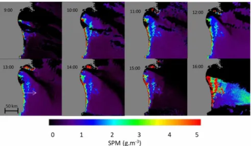
Figure 5 shows that SPM concentrations at 16:00 are high (greater than 5 g m-3) offshore in a large oceanic area. It is likely that these SPM concentration values are over-estimated because of the high sun zenith angle (71.55°) at this time of the day. Such a high sun zenith angle prevents the light from entering the water column. Therefore, the satellite data acquired at 16:00 are unreliable to be further used in this study. The SPM patterns observed are fairly stable in space over the course of the day (from 9h to 15h). The superimposition of the images indicated a maximum shift of 2 pixels (1 km) between the patterns from one image to another (not shown).

MERIS and MODIS sensors have also observed the same phenomenon as that observed in Figure 4, but with only one image per day because of their sun-synchronous orbit. MODIS acquired one image on March 13, 2011 and the first exploitable MERIS image available after the tsunami was acquired on March 17 (Figure 6). The low revisit period of these sun- synchronous sensors is a drawback. However, MODIS data show similar patterns to those observed in the GOCI image. Although the MERIS image is cloudier, the SPM patterns are still visible.

Figure 5: SPM concentrations obtained with GOCI satellite data (8 images per day) acquired on March 12, 2011 (i.e., the day after the tsunami).

GOCI, March 12 MODIS, March 13 MER1S, March 17

0 1 2 3 4 5

SPM (g.nr3)

Figure 6: SPM concentrations obtained with GOCI, MODIS and MERIS on the same area between March 12 and 17, 2011

A spatial transect showing the variation of the SPM at latitude

37.541° from the coastline to 64 km offshore, (see the arrow in GOCI image acquired at 13:00 in Figure 5) has been studied for various days from March 6 to March 28, 2011 (Figure 7). Note that the turbidity was weak (less than 0.5 g.m-3) along the transect just before the tsunami (March 6).

The day after the tsunami (March 12), the spatial variation of

SPM exhibits four peaks of turbidity, which occur at 2, 14, 25

and 37 km from the coastline respectively. It is interesting to note that the peaks are regularly spaced with a distance of about 12 km between each of them. The first SPM peak value is 8 times larger than the SPM concentration observed the day of the tsunami (4.4 g.m-3 against 0.5 g m-3). In addition, the peak of turbidity is about 2 km stretched spatially. The second peak shows an SPM value of 1.8 g.m-3 and extends over a width of 3 km. The two last SPM peaks show values of 1.0 g.m-3 with a wider spatial extension (about 5 km wide). Therefore, the maximum value of the SPM peaks decreases away from the coastline while their spatial width increases.

A week after the tsunami (on March 18), the first SPM peak value remains significant (3.8 g.m-3). However, the SPM variation becomes stable beyond 10 km, with SPM concentration values of about 1 g m-3. Two weeks after the tsunami (on March 28), the turbidity regularly decreases from 2.3 g.m-3 near the coast to 0.5 g.m-3 beyond 20 km.

The slope of the bathymetry is weak up to 45 km from the shore prior to significant increases, thus highlighting the limit of the continental shelf. Such a bathymetry variation will be used later to partly explain the origin of the SPM.

Figure 7: Spatial variation of the SPM concentration as derived by the GOCI over a West-East transect (latitude 37.541 °, 64 km wide) for various days between March 6 and March 28, 2011. The bathymetry shown in Figure 2 is also reported (green line).

B. Evolution of the SPM concentration in the Bay of Sendaï between March 5 and May 25, 2011

The temporal variation of SPM concentration in the Bay of Sendaï (red area in Figure 4) over a period of 3 months, namely between March 5, 2011 and May 25, 2011, is examined (Figure 8). The amount of rainfall measured at Fukushima city station (37.76°N and 140.47°E) is also shown in Figure 8.

Interestingly, each rainfall occurrence is often followed by an increase in SPM in the Bay of Sendaï. As examples, the rainfall

that is observed on March 8 or March 25 is consistent with an increase in SPM on March 10-12, and April 1, respectively. This is likely due to the Abukuma River discharges in the Bay. It is also observed that the mean SPM concentration increases by more than a factor of 3 just after the tsunami from 0.5 to 1.75 g.m-3 in the Bay of Sendaï. Then, the SPM decreases to 0.65 g.m-3 on April 12, 2011 until a substantial increase, up to 3.5 g.m-3 which occurs a few days after two heavy rainfalls that occurred on April 19 and 23.

Figure 8: Temporal variation of the SPM concentration in the Bay of Sendaï (blue) and the amount of rainfall measured at the Fukushima city station (orange) between March 5 and May 25, 2011

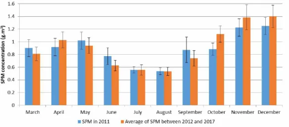
C. Comparison of monthly average SPM concentration in the Bay of Sendaï between (year) 2011 and the period 2012-2017

In this section, the monthly average SPM concentration observed in the Bay of Sendaï in 2011 is compared with the monthly average SPM concentration that has been estimated for the time period [2012-2017] to investigate whether the SPM concentration shows an increase during the specific year of the tsunami as it was previously observed for the tsunami of Sumatra in 2004 [9]. Unfortunately, although the GOCI was launched in 2010, no data are available before March 2011, thus preventing any comparison with data acquired prior to the

tsunami. As performed by [9] in 2009, the SPM concentration is averaged over each month and over six years after the tsunami event. The averages are then compared with the monthly averages observed in 2011 (Figure 9). The seasonal cycle of SPM concentration is noticeable: the minimum SPM concentration is reached in summer and the maximum in winter. A higher SPM concentration is observed in March, May, June and September 2011, than in the same months after 2012. The standard deviation of the SPM concentration seems to be correlated with the SPM average. The higher the SPM concentration, the higher the spatial variability.

IV. Discussion

The origin and the fate of the SPM using the geostationary images after the tsunami are now discussed.

Figure 5, Figure 7 and Figure 8 clearly show that the SPM concentration increases along the coast after the tsunami. The highest concentrations of SPM are located close to the coast, with a maximum of 11.1 g.m-3 in the south of the Bay of Sendaï on March 12, 2011 (10:00). Such an increase along the coast could be mostly ascribed to the tsunami since no significant rainfall was recorded before the earthquake (Figure 8). These high SPM loads can have different origins. First, they could originate from the land as a result of the return wave shape of the tsunami after the wave has reached the continent. Second, they could arise from the resuspension of the bottom sediment induced by the tsunami wave energy. These two oceanic processes seem to be combined and lead to the increase in SPM a few moments after the tsunami.

Figure 7 shows other SPM concentration peaks located at 14, 25 and 37 km from the shore. One may assume that the SPM hydrosols that are responsible for these peaks originate from the coast. If such an assumption is true, this means that the transport of SPM away from the coast and toward offshore would have happened rapidly, typically with a speed of about 2 km h-1 (i.e., covering 40 km in 19 hours). In addition, such transport, which also corresponds to a coverage of 12 km in 6 h (from 9:00 to 15:00) (i.e. 24 GOCI pixels), would be easily observable in Figure 5. However, between 9:00 and 15:00, the SPM patterns do not show any significant transport as mentioned in section 2.A (i.e., the patterns vary only slightly (by 2 pixels) over the course of the day). Therefore, the hydrosols could not originate from the coast. Another possible mechanism could be that the

SPM is re-suspended from the bottom through an upward

migration of the material towards the sea surface. The analysis of the bathymetric features of the study area and of the tsunami characteristics is consistent with the amount of SPM at quasi- periodic locations along the transect shown in Figure 7.

According to [43], the Tohoku tsunami wave energy was strongly reflected at the coast, partially trapped on the coastal shelf and directed back to the coast, resulting in extensively repeated tsunami attacks. This phenomenon can be explained as follows. At latitude 37.541°N (Figure 7), the bottom depth slowly increases from 50 m to 150 m up to 48 km offshore. The period of the tsunami wave train (denoted T) is about 13 min [2]. The tsunami’s wavelength depends on the depth as follows (Eq. 5):

A = (Eq. 5)

where h is the bottom depth and g is the gravitational acceleration. The wavelengths then correspond to 17, 24 and 30 km when the sea bottom depth is 50, 100 and 150 m respectively.

Because the coastal shelf width of the study area (48 km) is about twice the mean tsunami wavelength (23.6 km), which corresponds to near resonance conditions for the tsunami waves, the reflection of the wave on the coast causes the progressive wave of the tsunami to become a standing

(stationary) wave, alternatively reflected by the coast and the coastal shelf.

It is worth noting that the near-bed velocity of a standing wave is twice as high under the nodes compared to the near-bed velocity of a progressive wave. For a progressive wave of 2m in height and a bottom depth of 150 m, the near-bed maximum velocity under the node is about 25 cm.s-1 (eq. 4), while the near-bed maximum velocity of a standing wave is about 50 cm.s-1. The four SPM peaks observed in Figure 7, showing a spacing of about half the tsunami’s wavelength (12 km) correspond to the four anti-nodes of the standing wave, where the speed is essentially vertical. The recirculation cells tend to make the particles migrate vertically. At the nodes, the sedimentation is the highest where the horizontal oscillation velocity of the fluid is maximal. Therefore, the sea-bed velocity increases as the depth decreases. The highest peak concentration (4.3 g.m-3) is indeed observed near the coast where bathymetry is the lowest. This result confirms the study [45] dealing with the reflection of the tsunami wave on the Bay of Sendaï coastline. Strong ground motions induced by the earthquake followed by high frictional velocities of the subsequent tsunami would have contributed to high concentrations of SPM in the water column above the shelf. The collapse of the water column generated the turbidity current that formed the offshore deposit. If part of the sediment is transported by turbidity currents and settles on the outer terrace as mentioned by [46], a certain amount is re-suspended up to the near surface, as observed with GOCI data. Ikehara et al. [44] also observed such a phenomenon. The high frictional velocities associated with the tsunami are likely to have influenced the seafloor and surface sediments, especially in shallow water areas. They also collected an undisturbed surface sediment sample from the outer shelf of the Bay of Sendaï, which revealed evidence of strong ground shaking associated with the earthquake and agitation by subsequent tsunami waves. Ground shaking resulted in the deformation of unconsolidated sediment, and also contributed to the resuspension of diatomaceous surface sediments. The high frictional velocities that occur when tsunami waves propagate into shallow water [45] resuspended muddy shelf sediments on the Sendaï Shelf, thus creating a water column with a high concentration of suspended sediment. The collapse of this column resulted in the repeated generation of turbidity currents on the outer shelf.

The evolution of the SPM concentration in the Bay of Sendaï over a longer period, taking into account the rainfalls measured at the Fukushima city station between March 5 and May 25 (Figure 8), has been examined above. Several studies analyzed the influence of rainfalls on the SPM concentration. Rao et al. [46] collected SPM at regular stations from the Mandovi and Zuari estuaries; their results showed that the peaks of high SPM are consistent with peaks of high rainfall and low salinity but also with peaks of moderate/low rainfall coupled with high salinity during the monsoon. In the Mekong River, previous studies suggested that the turbidity is likely to have been caused by extremely high runoff and consequent rising water levels due to heavy rainfall. Turbidity usually increases sharply during heavy rainfall when particles from the soil surface are washed into the river and the river bed sediment is re-suspended [47]. Here, it was shown that all rainfalls are followed by an increase

in SPM concentration, except after the tsunami (Figure 8). Figure 8 is also useful to monitor the lowest SPM concentration values without rainfalls. If a 4-day lag SPM is compared with rainfall, a correlation does exist (R2=0.4148). The rainfall plays a significant role in increasing the amount of SPM at the surface level after 4 days.

Between March 5 and May 25, the SPM concentration decreased rapidly. More than two weeks after the tsunami, the concentration remains spatially homogeneous around 0.5 g.m-3 (Figure 7), though it is still above the concentration level observed before the tsunami (around 0.13 g m-3). The mean

SPM concentration observed in the Bay of Sendaï after the

tsunami also remains systematically greater (at least 0.65 g m- 3) than the concentration observed before the tsunami (around 0.5 g m-3) (Figure 8). This means that although some of the hydrosols (heavy particles) probably settled, the lightest ones have been scattered in the ocean and the SPM hydrosols linked with the occurrence of the tsunami are still in suspension in the water column almost 3 months later.

Finally, the SPM monthly concentrations observed in 2011 were compared to the observations made over a period of six years after the tsunami, as it was previously carried out for the Sumatra tsunami in 2004 by [9]. Interestingly, the increase in the SPM concentration of 55.5 to 200%, which was observed just after the Sumatra tsunami and which led to an increase in

SPM concentration over the entire North East Indian Ocean,

was not observed here. In addition, an increase in SPM concentration was observed (from 4.3 to 6.2%) in the entire North East Indian Ocean in 2005 when compared to the 5-year monitoring period (2002-2006) [8]. The gOcI data, and thus the variation of the SPM concentrations, were not available for the years prior to the Tohoku tsunami. The monthly SPM concentration derived in 2011 is higher than the average calculated for the months over the 2012-2017 time period only in March, May, June and September (figure 9). This can be explained by the higher input of SPM in the ocean after each rainfall compared to years without tsunami because SPM in river and watershed are more present at the surface after a tsunami. The Tohoku Tsunami also had a similar influence on the SPM concentration to the one induced by the tsunami of Sumatra in 2004 but not for such a long period.

Buesseler et al. [3] highlighted that only a small fraction of the FDNPP-derived radiocesium associated with particulate organic matter and clay particles accumulated on the seafloor. The majority of the FDNPP-derived radionuclides were mixed and diluted quite rapidly in the rough waters off the coast of Japan under the influence of currents, tidal forces, and eddies, with the major flow of the contaminated plume moving eastward under the influence of the southward-flowing Oyashio Current and the stronger, northward- and eastward-flowing Kuroshio Current. Therefore, it is likely that the SPM was both settled and scattered by the currents during the tsunami event.

V. Conclusion

In this study, the spatio-temporal variation of the SPM concentration was investigated at various time scales after the tsunami which occurred in Japan in 2011. One day after the tsunami, patterns of SPM concentrations were observed in

GOCI satellite data. The analysis showed that the hydrosols likely originate from the resuspension of bottom sediments due to the influence of the reflection of the tsunami on the coastline that leads to the migration of marine particles towards the sea surface. The SPM concentration rapidly decreases two weeks after the tsunami. However, the concentrations remain higher than those observed before the tsunami event. Only one month after the tsunami the amount of SPM reverted to similar concentrations to those observed before the earthquake. Finally, it was shown that the monthly averaged SPM concentration observed in 2011 was higher than that observed over a period of 6 years after the tsunami, but only for a 6-month period while a long term increase of SPM (i.e., longer than 6 months) was observed after the tsunami of Sumatra in 2004.

Acknowledgment

This research was supported by the French program “Programme Investissement d’Avenir” run by the National Research Agency. (AMORAD project, grant ANR-11-RSNR- 0002). The authors are also grateful to the Korean Ocean Satellite Center (KOSC) for providing the GOCI imagery. They also would like to thank the anonymous reviewers for their relevant comments and suggestions.

REFERENCES

[1] W. Yong, L. Yanping, et S. Youpo, « The Study of Japan Earthquake Deformation Based on GPS », Procedia Environ. Sci., vol. 10, p. 9-13, 2011. [2] Y. Fujii, K. Satake, S. Sakai, M. Shinohara, et T. Kanazawa, « Tsunami source of the 2011 off the Pacific coast of Tohoku Earthquake », Earth Planets

Space, vol. 63, no 7, p. 55, 2011.

[3] K. Buesseler et al., « Fukushima Daiichi-derived radionuclides in the ocean: transport, fate, and impacts », Annu. Rev. Mar. Sci., vol. 9, p. 173-203, 2017. [4] C. Stan-Sion, M. Enachescu, et A. Petre, « AMS analyses of I-129 from the Fukushima Daiichi nuclear accident in the Pacific Ocean waters of the Coast La Jolla-San Diego, USA », Environ. Sci. Process. Impacts, vol. 17, no 5, p. 932-938, 2015.

[5] B. Qiu, Kuroshio and Oyashio currents. Academic Press, 2001.

[6] K. O. Buesseler et al., « Fukushima-derived radionuclides in the ocean and biota off Japan », Proc. Natl. Acad. Sci., vol. 109, no 16, p. 5984-5988, 2012. [7] O. Evrard et al. , Evolution of radioactive dose rates in fresh sediment

deposits along coastal rivers draining Fukushima contamination plume, Scientific reports, 3, 3079. 2013.

[8] N. Anilkumar, Y. Sarma, K. Babu, M. Sudhakar, et P. Pandey, « Post­ tsunami oceanographic conditions in southern Arabian Sea and Bay of Bengal », Curr. Sci., vol. 90, no 3, p. 421-427, 2006.

[9] Z. Yan et D. Tang, « Changes in suspended sediments associated with 2004 Indian Ocean tsunami », Adv. Space Res., vol. 43, no 1, p. 89-95, 2009. [10] X. Zhang, D. Tang, Z. Li, et F. Zhang, « The effects of wind and rainfall on suspended sediment concentration related to the 2004 Indian Ocean tsunami », Mar. Pollut. Bull., vol. 58, no 9, p. 1367-1373, 2009.

[11] R. Singh, S. Bhoi, et A. Sahoo, « Changes observed in land and ocean after Gujarat earthquake of 26 January 2001 using 1RS data », Int. J. Remote

Sens., vol. 23, no 16, p. 3123-3128, 2002.

[12] S. Kundu, A. Sahoo, S. Mohapatra, et R. Singh, « Change analysis using IRS-P4 OCM data after the Orissa super cyclone », Int. J. Remote Sens., vol. 22, no 7, p. 1383-1389, 2001.

[13] V. K. Agarwal, N. Agarwal, et R. Kumar, « Simulations of the 26 December 2004 Indian Ocean tsunami using a multi-purpose Ocean disaster simulation and prediction model », Curr. Sci., p. 439-444, 2005.

[14] S. Singh et al., « A preliminary report on the Tecomân, Mexico earthquake of 22 January 2003 (Mw 7.4) and its effects », Seismol. Res. Lett., vol. 74, no 3, p. 279-289, 2003.

[15] V. Singh, « Impact of the Earthquake and Tsunami of December 26, 2004, on the groundwater regime at Neill Island (south Andaman) », J. Environ.

Manage., vol. 89, no 1, p. 58-62, 2008.

[16] R. Sarangi, « Remote sensing of chlorophyll and sea surface temperature in Indian water with impact of2004 Sumatra tsunami », Mar. Geod., vol. 34, no 2, p. 152-166, 2011.

[17] R. K. Sarangi, « Impact assessment of the Japanese tsunami on ocean- surface chlorophyll concentration using MODIS-Aqua data », J. Appl. Remote

Sens., vol. 6, no 1, p. 063539, 2012.

[18] P. Curran, J. Dash, et G. Llewellyn, « Indian Ocean tsunami: The use of MERIS (MTCI) data to infer salt stress in coastal vegetation », Int. J. Remote

Sens., vol. 28, no 3-4, p. 729-735, 2007.

[19] M. Arii, M. Koiwa, et Y. Aoki, « Applicability of SAR to marine debris surveillance after the Great East Japan Earthquake », IEEE J. Sel. Top. Appl.

Earth Obs. Remote Sens., vol. 7, no 5, p. 1729-1744, 2014.

[20] C. O. Dumitru, S. Cui, D. Faur, et M. Datcu, « Data analytics for rapid mapping: Case study of a flooding event in Germany and the tsunami in Japan using very high resolution SAR images », IEEE J. Sel. Top. Appl. Earth Obs.

Remote Sens., vol. 8, no 1, p. 114-129, 2015.

[21] K. Goto, K. Ikehara, J. Goff, C. Chagué-Goff, et B. Jaffe, « The 2011 Tohoku-oki tsunami—Three years on », Mar. Geol., vol. 358, p. 2-11, 2014. [22] J.-K. Choi, Y.-J. Park, B. R. Lee, J. Eom, J.-E. Moon, et J.-H. Ryu, « Application of the geostationary ocean color imager (GOCI) to mapping the temporal dynamics of coastal water turbidity », Remote Sens. Environ., vol.

146, no 0, p. 24-35, 2014.

[23] D. Doxaran et al., « Retrieval of the seawater reflectance for suspended solids monitoring in the East China Sea using MODIS, MERIS and GOCI satellite data », Remote Sens. Environ., vol. 146, no 0, p. 36-48, 2014. [24] X. He et al., « Using geostationary satellite ocean color data to map the diurnal dynamics of suspended particulate matter in coastal waters », Remote

Sens. Environ., vol. 133, p. 225-239, 2013.

[25] X. Lou et C. Hu, « Diurnal changes of a harmful algal bloom in the East China Sea: Observations from GOCI », Remote Sens. Environ., vol. 140, no 0, p. 562-572, 2014.

[26] M. Wang et al., « Ocean color products from the Korean Geostationary Ocean Color Imager (GOCI) », Opt. Express, vol. 21, no 3, p. 3835-3849, févr. 2013.

[27] S. Haruyama et T. Sugai, Natural Disaster and Coastal Geomorphology. Springer, 2016.

[28] C. Chartin et al., « Tracking the early dispersion of contaminated sediment along rivers draining the Fukushima radioactive pollution plume »,

Anthropocene, vol. 1, p. 23-34, 2013.

[29] I. Ioc, « BODC, 2003. Centenary Edition of the GEBCO Digital Atlas, published on CD-ROM on behalf of the Intergovernmental Oceanographic Commission and the International Hydrographic Organization as part of the General Bathymetric Chart of the Oceans », Br. Oceanogr. Data Cent. Liverp.

UK, vol. 260, 2008.

[30] J. H. Ahn, Y. J. Park, J. H. Ryu, B. Lee, et I. S. Oh, « Development of atmospheric correction algorithm for Geostationary Ocean Color Imager (GOCI) », Ocean Sci. J., vol. 47, no 3, p. 247-259, 2012.

[31] M. Lei, A. Minghelli, M. Fraysse, I. Pairaud, R. Verney, et C. Pinazo, « Geostationary image simulation on coastal waters using hydrodynamic biogeochemical and sedimentary coupled models », IEEE J. Sel. Top. Appl.

Earth Obs. Remote Sens., vol. 9, no 11, p. 5209-5222, 2016.

[32] H. R. Gordon et M. Wang, « Influence of oceanic whitecaps on atmospheric correction of ocean-color sensors », Appl. Opt., vol. 33, no 33, p. 7754-7763, 1994.

[33] G. Neukermans, K. Ruddick, E. Bernard, D. Ramon, B. Nechad, et P. Y. Deschamps, « Mapping total suspended matter from geostationary satellites: a easiblility study with SEVIRI in the Southern Norht Sea », Opt. Express, vol. 17, p. 14029-14052, août 2009.

[34] K. G. Ruddick, V. De Cauwer, Y.-J. Park, et G. Moore, « Seaborne measurements of near infrared water-leaving reflectance: The similarity spectrum for turbid waters », Limnol. Oceanogr., vol. 51, no 2, p. 1167-1179, 2006.

[35] B. Nechad, K. G. Ruddick, et Y. Park, « Calibration and validation of a generic multisensor algorithm for mapping of total suspended matter in turbid waters », Remote Sens. Environ., vol. 114, no 4, p. 854-866, 2010.

[36] A. I. Dogliotti, K. Ruddick, B. Nechad, D. Doxaran, et E. Knaeps, « A single algorithm to retrieve turbidity from remotely-sensed data in all coastal and estuarine waters », Remote Sens. Environ., vol. 156, p. 157-168, 2015. [37] A. Minghelli, M. Guillaume, P. Deliot, R. Marion, et M. Peirache, « Cartographie des fonds marins à partir d’images hyperspectrales aériennes par correction de l’atténuation du signal du fond par la colonne d’eau », Colloq.

Hyperspectral Grenoble, 2016.

[38] A. Morel et S. Bélanger, « Improved detection of trubid waters from ocean color sensors information », Remote Sens. Environ., vol. 102, p. 237-249, 2006.

[39] Z. Lee, K. L. Carder, et R. A. Arnone, « Deriving inherent optical properties from water color: A multiband quasi-analytical agorithm for optically deep waters », Appl. Opt., vol. 41, no 27, p. 5755-5772, 2002. [40] Z. Lee, K. L. Carder, C. D. Mobley, R. G. Steward, et J. S. Patch, « Hyperspectral remote sensing for shallow Waters. I. A semianalytical model », Appl. Opt., vol. 37, no 27, p. 6329-6338, 1998.

[41] A. Minghelli, M. Lei, et charmasson, Sabine, « Monitoring of Suspended Particulate Matter with GOCI on the Fukushima coast after the tsunami and the nuclear power plant accident (March 2011) », présenté à Ocean Optics, 2016, Victoria, Canada, 2016.

[42] M. T. Satria, B. Huang, T.-J. Hsieh, Y.-L. Chang, et W.-Y. Liang, « GPU acceleration of tsunami propagation model », IEEE J. Sel. Top. Appl. Earth

Obs. Remote Sens., vol. 5, no 3, p. 1014-1023, 2012.

[43] S. Sato, « Characteristics of the 2011 Tohoku Tsunami and introduction of two level tsunamis for tsunami disaster mitigation », Proc. Jpn. Acad. Ser.

B, vol. 91, no 6, p. 262-272, 2015.

[44] K. Ikehara, T. Irino, K. Usami, R. Jenkins, A. Omura, et J. Ashi, « Possible submarine tsunami deposits on the outer shelf of Sendai Bay, Japan resulting from the 2011 earthquake and tsunami off the Pacific coast of Tohoku », Mar. Geol., vol. 358, p. 120-127, 2014.

[45] D. Sugawara et K. Goto, « Numerical modeling of the 2011 Tohoku-oki tsunami in the offshore and onshore of Sendai Plain, Japan », Sediment. Geol., vol. 282, p. 110-123, 2012.

[46] V. P. Rao et al., « Suspended sediment dynamics on a seasonal scale in the Mandovi and Zuari estuaries, central west coast of India », Estuar. Coast.

Shelf Sci., vol. 91, no 1, p. 78-86, 2011.

[47] D. Thi Ha, S. Ouillon, et G. Van Vinh, « Water and Suspended Sediment Budgets in the Lower Mekong from High-Frequency Measurements (2009­ 2016) », Water, vol. 10, no 7, p. 846, 2018.