Spaceborne estimate of atmospheric CO$_2$ column by use of the differential absorption method: error analysis

HAL Id: hal-03121045

https://hal.archives-ouvertes.fr/hal-03121045

Submitted on 6 May 2021

HAL is a multi-disciplinary open access

archive for the deposit and dissemination of sci-entific research documents, whether they are pub-lished or not. The documents may come from teaching and research institutions in France or abroad, or from public or private research centers.

L’archive ouverte pluridisciplinaire HAL, est destinée au dépôt et à la diffusion de documents scientifiques de niveau recherche, publiés ou non, émanant des établissements d’enseignement et de recherche français ou étrangers, des laboratoires publics ou privés.

Spaceborne estimate of atmospheric CO_2 column by

use of the differential absorption method: error analysis

Emmanuel Dufour, François-Marie Bréon

To cite this version:

Emmanuel Dufour, François-Marie Bréon. Spaceborne estimate of atmospheric CO_2 column by use of the differential absorption method: error analysis. Applied optics, Optical Society of America, 2003, 42 (18), pp.3595-3609. �10.1364/AO.42.003595�. �hal-03121045�

Spaceborne estimate of atmospheric CO

₂

column

by use of the differential absorption method:

error analysis

Emmanuel Dufour and Franc¸ois-Marie Bre´on

For better knowledge of the carbon cycle, there is a need for spaceborne measurements of atmospheric CO2concentration. Because the gradients are relatively small, the accuracy requirements are better

than 1%. We analyze the feasibility of a CO2-weighted-column estimate, using the differential

absorp-tion technique, from high-resoluabsorp-tion spectroscopic measurements in the 1.6- and 2-␮m CO2absorption

bands. Several sources of uncertainty that can be neglected for other gases with less stringent accuracy requirements need to be assessed. We attempt a quantification of errors due to the radiometric noise, uncertainties in the temperature, humidity and surface pressure uncertainty, spectroscopic coefficients, and atmospheric scattering. Atmospheric scattering is the major source of error关5 parts per 106_共ppm兲

for a subvisual cirrus cloud with an assumed optical thickness of 0.03兴, and additional research is needed to properly assess the accuracy of correction methods. Spectroscopic data are currently a major source of uncertainty but can be improved with specific ground-based sunphotometry measurements. The other sources of error amount to several ppm, which is less than, but close to, the accuracy requirements. Fortunately, these errors are mostly random and will therefore be reduced by proper averaging. © 2003 Optical Society of America

OCIS codes: 120.0280, 010.1280, 120.6200.

1. Introduction

The rise of atmospheric CO2, the primary

anthropo-genic contribution to the greenhouse effect, is docu-mented at many observing sites around the world.1

Over the past 200 years, CO₂ concentration has in-creased by 30% in response to industrial emissions

and land-use change. Climate models predict a

global warming between 1.5 °C and 4 °C, for a dou-bling of the current concentration. To make reliable predictions of future CO2levels and set up apposite

CO₂ emission–mitigation strategies, it is of para-mount importance to quantify the factors that control atmospheric CO₂.

Observations over the past decades indicate that, on average, only approximately half of the anthropo-genic emissions end up being stored in the

atmo-sphere; the rest is reabsorbed by two natural reservoirs: the oceans and the continental bio-sphere.2 _{Net CO}

2removals by these two sinks have

different time scales. Carbon dissolved in the oceans has a time scale of several hundred years, whereas carbon taken up by trees and soils is stocked only for a few years, with a residence time depending on the type of ecosystem. To predict the future rate of increase of atmospheric CO₂concentration, there is a strong need to quantify carbon sources and sinks at a regional scale共i.e., finer than a 106_km2_兲.

It is possible to infer the spatial distribution of the carbon sources and sinks by using repeated CO₂ mea-surements on a global network of observatories. The atmosphere is a powerful integrator of the sur-face fluxes at large scale, which makes it possible to relate small but persistent concentration gradients to sources and sinks, provided that the air-mass trans-port is known. Hence atmospheric transport models can be used to interpret atmospheric measurements

in terms of surface fluxes by using inverse

methods.3–5 _{At present, the atmospheric CO} 2

obser-vation network consists of approximately 100 ground stations around the globe providing in situ concen-tration measurements 关with flasks or infrared 共IR兲 analyzers兴. In addition, a few vertical profiles are

The authors are with Laboratoire des Sciences du Climat et de l’Environnement, Direction des Sciences de la Matie`re, Commis-sariat a` l’Energie Atomique, 91191 Gif sur Yvette, France. The e-mail address of E. Dufour is dufour@lsce.saclay.cea.fr.

Received 29 November 2002; revised manuscript received 21 February 2003.

0003-6935_{兾03兾183595-15$15.00兾0} © 2003 Optical Society of America

acquired from airborne measurements. Unfortu-nately, the limited horizontal density and uneven distribution of the current network hinders the geo-location of the CO2fluxes at a resolution better than

the continent and ocean basin scales.6,7

Further-more, the current temporal frequency of the observa-tions used in the inversions共monthly averages of CO₂ data兲 is insufficient to capture sporadic sources, such as fires, whose signals get severely damped by atmo-spheric diffusion after approximately a week. Therefore there is a strong need for a sampling net-work with much denser coverage in space and time than currently achieved with the existing surface net-work, and this suggests the use of satellite-based observations. Simulations show that spaceborne measurements could dramatically improve the deter-mination of carbon fluxes, provided that the precision of the measurement is sufficient. As atmospheric CO₂is a long-lived gas, its background concentration is large compared with the spatial and temporal vari-ations that need to be measured. In an individual satellite measurement, a precision of better than 1% 关⬍3 parts per 106 _{共ppm兲兴 is needed to reasonably}

detect fluxes.8 _{Above a threshold of approximately 5}

ppm, there is no substantial gain in flux uncertainty reduction from that obtained with the current surface network. Ideally, a vertical profile would be desir-able, but a integrated amount or column-weighted amount is also valuable, provided that the lower troposphere contributes significantly.

Three main technologies can be envisioned to mon-itor the CO2concentration from space. 共1兲 Analysis of

CO₂emission bands in the thermal IR region such as conducted with measurements from the TIROS 共Tele-vision Infrared Operational Satellite兲 operational ver-tical sounder on board the National Oceanic and Atmospheric Administration’s series of polar meteoro-logical satellites.9 _{In the near future this technique}

will be applied to much higher spectral resolution ra-diometers10,11 _{such as the atmospheric infrared}

sounder, launched onboard the NASA Aqua platform, and the infrared atmospheric sounding interferometer to be launched onboard the Meterological Operational satellite. 共2兲 Active differential absorption, envi-sioned for the Celsius mission proposed, but not se-lected, for the NASA Earth System Science Pathfinder 3共ESSP-3兲 call.12 共3兲 Passive differential absorption,

measuring the solar light reflected by the Earth’s sur-face after a double atmospheric path. This method is

used with the SCIAMACHY 共scanning imaging

ab-sorption spectrometer for atmospheric chartography兲 instrument, onboard the Environmental Satellite 共EN-VISAT兲 platform and is envisioned for the Orbiting Carbon Observatory mission, recently selected in the NASA ESSP-3 call. In the scope of this paper we propose to focus on an instrumental concept reliant on the last technique.

From the ground, the determination of atmospheric gas column abundance by using direct sunlight is a mature technique. By reanalyzing high-resolution spectra records measured at the Kitt Peak National Solar Observatory, Yang et al.13 _retrieved

column-averaged amounts of CO₂with a precision better than 0.5%. For satellite-based measurements, the ques-tion is whether an individual precision of 1% is feasi-ble. In recent years, several sensitivity studies have investigated the attainable precision of the sunlight-based technique with a spaceborne instrument. Tol-ton and Plouffe14 _{have considered a radiometer}

consisting of 22-cm⫺1-wide bandpass filters tuned around the 1.6-␮m CO₂band. Buchwitz et al.15_have

evaluated the potential of the SCIAMACHY spectrom-eter, which provides 0.5-cm⫺1spectral resolution scans in a 250-cm⫺1-wide window around the 2.0-␮m CO2

band. O’Brien and Rayner16_{have focused on the}

er-ror due to undetected atmospheric scattering by opti-cally thin cirrus and aerosol. They propose a procedure by which the scattering problem may be overcome by using simultaneous measurements at se-lected wave numbers around 1.6 ␮m and an oxygen band around 1.27 ␮m. Finally, in an introductory study, Kuang et al.17 _{projected the retrieval of}

atmo-spheric CO₂by using three short-wavelength infrared 共SWIR兲 spectrometers operating in the A band at 0.76 ␮m, and in the 1.6- and 2.0-␮m CO2bands, indicating

a potential accuracy of 0.3–2.5 ppm. The 0.76-␮m band is used to correct for the effect of atmospheric scattering on the measurement. This oxygen band was chosen rather than the 1.27-␮m band suggested by O’Brien and Rayner16_{because the latter is strongly}

affected by airglow and therefore appears to be unus-able for scattering correction unless the measurements are made at high spectral resolution as proposed by O’Brien and Rayner.16 _{In the present paper we}

in-vestigate the CO₂column inversion from the analysis of high-resolution spectra in optimized microwindows at 1.6 and 2.0␮m. We attempt to list and quantify all uncertainty sources individually to provide a detailed budget of baseline errors and propose potentials for error reduction. We first recall the principle of differ-ential absorption spectroscopy, then we propose an op-timized instrument and retrieval algorithm designed for the recovering of CO₂column abundance, and, fi-nally, we discuss the sources of incertitude.

2. Measurement Principle A. General Theory

The measuring principle共Fig. 1兲 relies on the spectral analysis of the solar radiance reflected on the Earth’s surface back to the top of the atmosphere 共TOA兲 in the SWIR domain. In the measured spectrum, each atmospheric molecular species leaves a characteristic set of absorption lines by which it can be identified and quantified, provided that the spectral resolution is adequate. In the absence of scattering by the at-mosphere, the radiance L reflected to space is propor-tional to the TOA atmospheric transmittance tatm

according to

L⫽ Es␮sRsurftatm兾␲, (1)

where the other parameters are defined in Table 1. Let k共␭, P, T兲 be the molecular absorption coefficient

where ␭, P, and T, respectively, denote the wave-length, pressure, and temperature. The spectrum of transmission may be written as

tatm共␭兲 ⫽ exp

冋

兰

Psurf

r共P兲k共␭, P, T兲dP

册

where m is the air-mass factor, Nairis the number of

molecules of dry air in the atmospheric column per unit pressure, r is the volume mixing ratio of the gas, and P_surfdenotes the surface pressure.

The column-averaged volume mixing ratio, defined as the total mass of gas normalized by the total mass of air in an atmospheric column, is

r៮ ⫽ 1 Psurf

兰

Psurf

r共P兲dP. (3)

If we consider, in a first approximation, that the ab-sorption coefficient is constant with height, then, af-ter Eqs.共2兲 and 共3兲,

tatm共␭兲 ⫽ exp关⫺mNairk共␭兲 Psurfr៮兴, (4)

Fig. 1. CO2column estimation relies on the measurement of the

solar radiance reflected on the Earth’s surface back to the TOA. Atmospheric scattering, which allows photons to be measured that have not traversed the full double atmospheric path, is a source of bias for the column estimates.

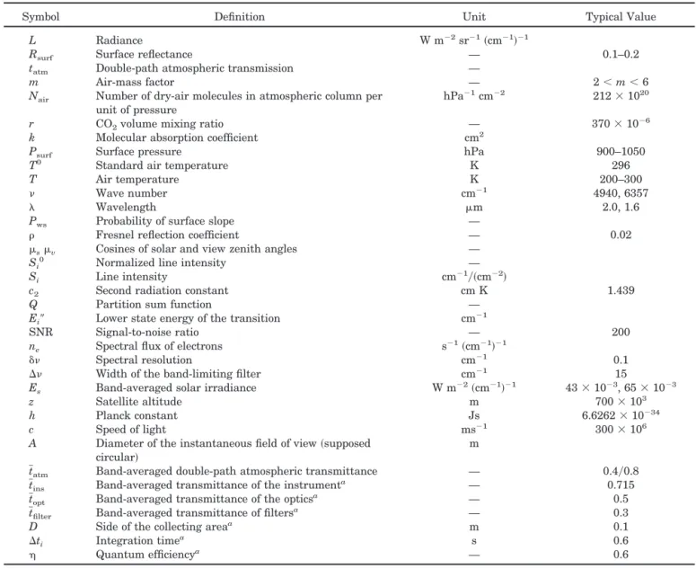
Table 1. Variables and Constants Used in This Paper Together with Typical Values When They Exist

Symbol Definition Unit Typical Value

L Radiance W m⫺2sr⫺1共cm⫺1兲⫺1

Rsurf Surface reflectance — 0.1–0.2

tatm Double-path atmospheric transmission —

m Air-mass factor — 2⬍ m ⬍ 6

Nair Number of dry-air molecules in atmospheric column per

unit of pressure

hPa⫺1cm⫺2 212⫻ 1020

r CO2volume mixing ratio — 370⫻ 10⫺6

k Molecular absorption coefficient cm2

Psurf Surface pressure hPa 900–1050

T0 _{Standard air temperature K 296}

T Air temperature K 200–300

␯ Wave number cm⫺1 4940, 6357

␭ Wavelength ␮m 2.0, 1.6

Pws Probability of surface slope —

␳ Fresnel reflection coefficient — 0.02

␮s␮v Cosines of solar and view zenith angles —

Si

0 _{Normalized line intensity —}

Si Line intensity cm⫺1兾共cm⫺2兲

c2 Second radiation constant cm K 1.439

Q Partition sum function —

Ei⬙ Lower state energy of the transition cm⫺1

SNR Signal-to-noise ratio — 200

ne Spectral flux of electrons s⫺1共cm⫺1兲⫺1

␦␯ Spectral resolution cm⫺1 0.1

⌬␯ Width of the band-limiting filter cm⫺1 15

Es Band-averaged solar irradiance W m⫺2共cm⫺1兲⫺1 43⫻ 10⫺3, 65⫻ 10⫺3

z Satellite altitude m 700⫻ 103

h Planck constant Js 6.6262⫻ 10⫺34

c Speed of light ms⫺1 300⫻ 106

A Diameter of the instantaneous field of view共supposed circular兲

m

t៮atm Band-averaged double-path atmospheric transmittance — 0.4兾0.8 t៮ins Band-averaged transmittance of the instrument

a _{— 0.715}

t៮opt Band-averaged transmittance of the optics

a _{— 0.5}

t៮filter Band-averaged transmittance of filters

a _{— 0.3}

D Side of the collecting areaa _{m 0.1}

⌬ti Integration time

a _{s 0.6}

␩ Quantum efficiencya _{— 0.6}

a_{Instrumental parameters values are the results of a spaceborne Fourier-transform spectrometer concept study conducted at Centre}

which reveals a quasi-linear relation between the log-arithm of the measured radiance and the column-averaged concentration, at a given wavelength. In practice, the absorption coefficient k varies along the atmospheric column through pressure and tempera-ture so the measurement depends not only on the total amount of gas but also on its vertical distribu-tion. The sensitivity to the CO2vertical distribution

共weighting function兲 will be established in Subsection 5.A.

Because the TOA radiance is also dependent on the surface reflectance through Eq.共1兲, at least two fre-quencies are needed for the concentration estimate. In the so-called differential absorption technique, the difference of optical depth between a sensitive fre-quency, chosen to lie near the center of an absorption line of the target species, and a nonsensitive fre-quency, outside the absorption line, is measured. In the proposed method this principle is extended to spectral measurements共differential absorption spec-troscopy兲. If the absorption is a good measure for the concentration of the target molecule, it is also driven by the other parameters in Eq. 共2兲 共surface pressure, temperature vertical profile, and air-mass factor兲. As these parameters are known only to a finite accuracy, they are potential sources of error, whose effect will be assessed further in Subsections 5.B to 5.F.

B. Main Limitations and Constraints

The principle of atmospheric column estimate by dif-ferential absorption requires that most of the mea-sured radiance goes through a full atmospheric path. Over the oceans, in the near IR, the only significant contribution to the surface reflectance is the glint. As a consequence, the instrument must point roughly toward the specular direction. The glint pattern de-pends on the wind speed and is typically of the order of a few to 20 deg. Thus the pointing tolerance is of the order of 1 deg. In Subsection 3.B we discuss the order of magnitude of glint reflectance over the oceans.

Another consideration is the cloud cover. A reli-able retrieval requires the absence of clouds in the instrument’s field of view. Thus the footprint size must be limited to minimize the probability of cloud contamination.

Finally, the measurements at low-elevation Sun angles must be avoided because共1兲 the incoming ir-radiance is then lower, which reduces the signal-to-noise ratio共SNR兲 and 共2兲 the atmospheric scattering contribution 共see Fig. 1兲 that is unwanted for the proposed method gets larger both because of a slant-path effect and because of the scattering phase func-tion. In practice, solar zenith angles 共SZAs兲 larger than 75 deg 共elevation angles less than 15 deg兲 are probably not usable.

C. Optimal Transmission

In the SWIR the atmospheric transmission spectrum is the result of overlapping H₂O and CO₂bands共Fig. 2兲. Favored regions are CO2absorption bands that

are less contaminated by the H2O absorption lines.

Using this approach, we identified two potential spec-tral regions around 1.6 and 2.0␮m.

After Eq.共4兲, for a single spectral grid-point mea-surement, a perturbation ⌬tatm of the measured

transmission, due to radiometric noise, would pro-duce a relative estimation error:

⌬r៮ r៮ ⫽ ⌬tatm tatm 1 ln共tatm兲 . (5)

The most favorable spectral elements are those that minimize the impact of radiometric noise. As dem-onstrated by Eq.共5兲, regions of transparent transmis-sion 共tatm close to 1兲 or with large absorptions 共tatm

close to 0兲 yield the largest retrieval errors. This suggests the need for a measurement at intermediate transmission. Typically, if we suppose the pertur-bation is caused by a spectrally white noise 共a

real-istic assumption for a Fourier-transform

spectrometer兲, the best-suited spectral elements are for t_atm⫽ 0.37, but a measurement is still acceptable for a large range of transmission around this optimal value 共the error does not degrade by more than a factor of 2 as long as 0.07 ⬍ tatm ⬍ 0.79兲.

3. Instrument Design

A. Orbit and Time of Acquisition

The satellite should be polar orbiting to provide a large coverage of the Earth. Owing to scattering in the atmosphere, low SZAs are needed for a proper measurement, which implies a local time of observa-tion around midday. This suggests the satellite should be launched on a Sun-synchronous orbit with equator-crossing time close to noon.

B. Viewing Geometry

Surface reflectance directly affects the quality of the CO₂retrievals. First, measurements benefit from a better SNR over bright surfaces. Second, high sur-face albedo limits the relative effect of scattering pro-cesses taking place in the atmosphere, as it decreases

Fig. 2. Simulated spectrum of atmospheric transmission in the SWIR region showing regions of CO2absorption around 1.6 and 2.0

␮m. In the calculation the densities of the absorbers in the at-mosphere were supposed to follow typical tropical profiles. The SZA and view zenithal angle共VZA兲 were set to 45 deg.

the proportion of the atmosphere-scattered rays over the surface-reflected ones. Over the oceans, the re-flectance consists of a diffuse component 共by

back-scattering of seawater mass兲 and a specular

component共Sun glint兲. Because water is highly ab-sorbing in the IR, the diffuse contribution is ex-tremely small 共less than 10⫺3兲 and therefore can hardly be used. The specular component of the re-flectance can be exploited but is significant only in the vicinity of the glint direction. The bidirectional glint reflectance Rsurfis related to Fresnel’s reflection

co-efficient␳ according to

Rsurf⫽ ␲*␳共i兲兾关4* cos4共␤兲␮s␮v兴Pws, (6)

where Pwsis the wave-slope distribution,␤ is the tilt

of the plane so inclined it would reflect the incident solar ray specularly to the satellite, and i is the angle of incidence of the ray on that plane. By use of the nondirectional approximation for the slope probabil-ity distribution proposed by Cox and Munk,19

Pws共␤兲 ⫽ 1兾共␲␴2兲exp关⫺tan2共␤兲兾␴2兴, (7)

where the variance␴2_{is related to the wind speed v}

共in meters per second兲:

␴2_{⫽ 0.003 ⫹ 5.12 ⫻ 10}⫺3_{v. (8)}

Figure 3 shows reflectances predicted by Eqs.共6兲–共8兲 in the specular direction共i.e., ␤ is null, and i is equal to the SZA兲 for typical oceanic wind stress and vari-ous Sun angles. The specular reflectance decreases with increasing wind speed共the glint pattern spreads out on rougher sea surfaces兲 and increases toward a large SZA with a marked ascent above 40 deg owing to the variation of Fresnel’s coefficient.

To assess the statistics of the Sun-glint intensity observed from a polar orbiting satellite, we used a database of clear-sky measurements of glint

reflec-tance observed by the spaceborne radiometer

POLDER20 共polarization and directionality of the

Earth’s reflectance兲 in the vicinity of the specular direction. The measured reflectances have been cor-rected for scattering by molecules and aerosols as well as gaseous absorption. The database consists of 37,074 glint reflectances and covers a wide range of

wind speed from approximately 1 to 15 m s⫺1and Sun angles as great as 55 deg. One should point out the relative dimness of the Sun glint for most of the ob-servations. As shown by the cumulative histogram in Fig. 4, 45% of the observed reflectances are below 0.1 and 85% are below 0.3. The average reflectance is 0.12, which is much smaller than cloud reflectance 共typically, 0.6兲. Figure 4 also presents cumulative histograms of the database subsets classified accord-ing to SZA. The observed magnitudes are in

agree-ment with the model prediction in Fig. 3.

Furthermore, the nonlinear behavior of the reflec-tance with SZA is perceptible共strong increase above 45 deg兲.

The direction of maximum reflectance is easily pre-dictable. It coincides roughly with the specular di-rection with a slight shift toward larger view zenithal angles 共VZAs兲 in the principal plane. Indeed, for a given SZA, facets inclined such that the angle of in-cidence is more grazing are relatively more reflecting 共the Fresnel coefficient increases with the angle of incidence兲. The direction follows a smooth and slow evolution with respect to the satellite referential. For a heliosynchronous satellite with an equatorial crossing time close to midnight or noon, the specular direction is close to the satellite forward or nadir plane at all times.

Over land, surface reflectance has a less marked directional signature so there is no particular con-straint on the viewing geometry. On the other hand, land reflectance varies strongly with wave-length and with the surface type. The

moderate-resolution imaging spectroradiometer 共MODIS兲

channels at 2.105–2.155 ␮m and 1.628–1.652 ␮m

give an indication of the reflectances at 2.0 and 1.6 ␮m, respectively. Cloud-free composite maps of surface reflectance produced with the spaceborne MODIS were analyzed for several types of surface cover. Figure 5 presents histograms of reflectance over a vegetated area共Amazonian forest兲, a snow-and ice-covered surface共Greenland兲, and a mineral surface共Sahara desert兲 at the wavelengths of inter-est. The average values around 2.0 and 1.6 ␮m

Fig. 3. Simulated glint reflectances in the specular direction as a function of wind speed for various SZAs␪s.

Fig. 4. Cumulative histograms of Sun-glint reflectance over ocean surface produced by POLDER. The histogram functions were computed from a complete database of 37,074 observations and different subsets of this database arranged by SZA␪s.

have been reported in a summary table 共Table 2兲 after empiric correction for the wavelength dispar-ity with the MODIS channels.

C. Spatial Resolution

Establishing the optimal satellite spot size results from a trade-off. Large spot size permits good SNR measurements but increases the probability of cloud contamination and the spatial heterogeneity in the instrument’s instantaneous field of view. Therefore the most favorable spot size is such that the SNR requirement is just met. Computation of the spec-trum SNR differs according to the type of interferom-eter.22 _{Typically, in the case of a Fourier-transform}

spectrometer, if we suppose the detectors are limited only by the Poisson statistics of discrete electron events, the band-averaged SNR is

SNR⫽ ne␦␯⌬ti兾共ne⌬␯⌬ti兲共1兾2兲, (9)

where neis the spectral flux of electrons.

When we assume that most of the photons arise from solar reflection, necan be written as a function

of the diameter A of the spot as

ne⫽ A2t៮inst៮optt៮filtert៮atmRsurfEs␮sD2␩兾共4z2hcv兲. (10)

Equations 共9兲 and 共10兲 permit us to relate the SNR and the spot size. As shown further in Subsection 5.B, the CO₂concentration rms error resulting from instrumental noise can be contained below 1 ppm by use of a SNR of 200共Fig. 8兲. If we assume the typical parameter values of Table 1, a need for a SNR of 200 would impose a spot size of approximately 5 km.

D. Spectral Interval Selection

In spaceborne atmospheric spectroscopy, it is com-mon for the measurement to be bound to small spec-tral regions, so-called microwindows, dedicated to the retrieval of the target species rather than to scan the whole absorption band. Establishing the microwin-dow spectral width is a subtle step in the design of the retrieval method. The extension of the spectral in-terval to a region in which the signal is sensitive to a change of the target parameter tends to decrease the overall retrieval error, provided that this does not occasion the increase of the number of unknown pa-rameters and that the additional spectral elements are little affected by the nontarget parameters.23

On the other hand, within narrow spectral intervals, parameters with broadband spectral signatures, such as scattering by aerosol and surface reflectance, the H2O continuum can be assumed constant.

Further-more, at a given sampling rate, a narrower spectrum will be acquired faster and thus less contaminated by the artifacts due to the spatial variation of surface reflectance, pressure, temperature profile, and gas abundances as the instrument’s instantaneous field of view moves across the Earth. In the present study we assume that the spectrometer scans are 15 cm⫺1wide.

The microwindow boundaries were adjusted in the previously identified CO2 absorption bands so as to

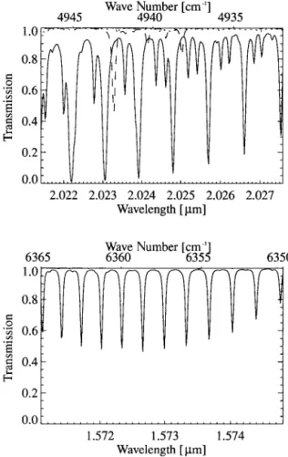
maximize the number of absorption lines within the bandwidth. As pointed out earlier, favored micro-windows contain prominent but nonsaturated ab-sorption lines of the target species. In addition, it was ensured that the spectral signature of the inter-fering species be minimum and noncorrelated to the target species’s signal. This finally led us to con-sider two optimized microwindows 共Fig. 6兲: 4932– 4947 cm⫺1共2.0214–2.0276 ␮m兲 and 6350–6365 cm⫺1 共1.5711–1.5748 ␮m兲, labeled, respectively, as the 2.0-and the 1.6-␮m channels in Subsection 3.E.

E. Spectral Resolution

As can be observed in the two simulated spectra of Fig. 6, the spectral interval between two consecutive strong CO2 transitions is of the order of 1 cm⫺1.

High spectral resolution and good knowledge of the instrument’s spectral response are required to sepa-rate the individual CO₂lines and resolve the atmo-spheric CO2 and H2O lines and solar lines. These

Fig. 5. Histograms of surface reflectance in cloud-free composite images produced by MODIS for the spectral bands 1.628 –1.652␮m 共dotted curve兲 and 2.105–2.155 ␮m 共solid curves兲 over different land surface covers. The two well-packed histograms are for the Amazonian forest. The two histograms with a maximum at 0.7 are for the desert. The two histograms with a broad distribution around 0.15 are for Greenland.

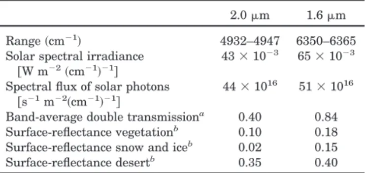
Table 2. Comparative Study of the Two Envisioned Spectral Windows

2.0␮m 1.6␮m Range_共cm⫺1_兲 4932–4947 6350–6365 Solar spectral irradiance

关W m⫺2_共cm⫺1_兲⫺1_兴

43_{⫻ 10}⫺3 65_{⫻ 10}⫺3 Spectral flux of solar photons

关s⫺1_m⫺2_共cm⫺1_兲⫺1_兴

44_{⫻ 10}16 _{51⫻ 10}16

Band-average double transmissiona _{0.40 0.84}

Surface-reflectance vegetationb _{0.10 0.18}

Surface-reflectance snow and iceb _{0.02 0.15}

Surface-reflectance desertb _{0.35 0.40} a_{Calculated by assuming the same atmosphere and observation}

geometry as for Fig. 6.

b_{Estimated after MODIS reflectance products at 2.105–2.155}

␮m and 1.628–1.652 ␮m 共Fig. 5兲. To account for the difference of wavelength with the MODIS channels, given values have been decreased by 5% to 60% in agreement with typical spectral profiles of land reflectance.21

observations have suggested the need for a spectral resolution of 0.1 cm⫺1共resolving power of 50,000兲 and a 0.05-cm⫺1 spectral sampling interval. Further-more, in the radiative transfer simulations below, the apodized instrument’s spectral response was as-sumed to have a Gaussian shape.

F. Advantages and Shortcomings of the Selected Intervals

Owing to larger CO₂ line intensities, the 2.0-␮m channel contains more spectral elements at interme-diate transmissions than the 1.6-␮m channel does. The 2.0-␮m channel appears better suited in this respect to capture the changes of CO₂ abundance. In addition, the sensitive spectral elements of the 2.0-␮m channel are located farther away from the line centers than those of the 1.6-␮m channel. Therefore inversion in the 2.0-␮m channel is driven by the regions of smoother slope and is then more robust with respect to incorrect spectral calibration 共shift or drift of the detectors兲 and uncertainties on

the instrument’s spectral response. On the other hand, the signal 共that is, the flux of photons from solar reflection兲 is expected to be larger in the 1.6-␮m channel. As shown in Table 2, the 1.6-␮m channel profits from higher flux of solar photons and a more transparent atmosphere. Furthermore, land sur-faces are usually brighter in the 1.6-␮m channel 共Ta-ble 2兲. Ocean reflectance is similar in the two bands. Though the retained microwindows are optimized in this regard, the 2.0-␮m channel suffers from sig-nificant H₂O contamination共Fig. 6兲. The inversion procedure supposes fixed vertical distribution of CO2

and H₂O concentrations, with variable total columns. The vertical profile of H2O is given by numerical

weather prediction共NWP兲 centers with significantly large error margins. Water-vapor content has large spatial and temporal variabilities in the atmospheric column. Although the H2O column is adjusted in

the inversion, uncertainty in the relative humidity profile could induce uncorrected error in the synthetic spectrum 共mostly through the alteration of the ab-sorption line shape兲.

Fraunhofer lines can be a potential source of error when they interfere with the atmospheric signatures in the measured spectrum. However, the spectral position of the Fraunhofer lines are well known from astronomic observations and can be screened off in the inversion procedure. On the basis of the high-resolution solar atlas produced by Livingston and Wallace,24_{we synthesized solar spectra degraded to}

the spectrometer resolution共0.1 cm⫺1兲 in the bands of interests共Fig. 6兲. Solar contamination remains lim-ited in both envisioned bands with relatively more prominent lines in the 1.6-␮m channel compared with the 2.0-␮m channel.

4. Error Analysis: Method and Models

Spaceborne sensing of CO₂poses a difficult challenge of accuracy: A satellite mission would be essentially worthless if the typical uncertainty on the retrievals was significantly larger than 1% 共3–4 ppm兲. For such required precision, many causes of uncertainty must be analyzed that could be neglected for other gases with lower requirements 共owing to a larger relative variability兲. The objective of this section and the next section is to draw up a complete error budget. Section 4 presents our general approach for assessing the error associated with a given parame-ter uncertainty and describes the forward and in-verse models used in this paper. In Section 5 we discuss and quantify the impacts of all the sources of uncertainty that we have identified.

A. General Approach

Let x be the state vector describing all the unknowns to be estimated from the measurement 共i.e., the column-averaged concentration of CO2 and several

by-products兲. We suppose that for a given x a for-ward model F can accurately produce a synthetic satellite measurement of TOA radiance spectrum

F共x, b兲, where b is a vector of model parameters that

Fig. 6. Spectral transmissions for the 2.0-␮m channel 共top兲 and the 1.6-␮m channel 共bottom兲, as simulated by our radiative trans-fer model. The CO2, H2O, and solar transmissions are shown by

the solid, dashed, and dotted lines, respectively. In the calcula-tion, CO2concentration was fixed to 370 ppm throughout the

at-mospheric column. The SZA and VZA were set to 45 deg. The solar spectrum was produced at the Kitt Peak National Observa-tory by the National Science Foundation, National Optical Astron-omy Observatories.

are not retrieved by the measurements共temperature profile, surface pressure, and spectroscopic data兲.

Furthermore, we consider an inverse model, I, which permits the exact restitution of x from the analysis of one spectrum, providing knowledge of the model parameters:

x⫽ I关F共x, b兲, b兴. (11)

In practice, the model parameters b are known only to a finite accuracy. Departures of the model param-eters from their assumed state induce an erroneous retrieval. Model parameters can be sources of ran-dom errors 共e.g., temperature兲 or systematic errors 共e.g., spectroscopic data兲. In our error analysis the retrieval error due to a given parameter was calcu-lated as follows. For a representative perturbation ⑀bof the parameter, the forward model produces an

altered spectrum F共x, b ⫹ ⑀_b兲. Then, assuming no perturbation, the altered spectrum is input through the inverse model to calculate the retrieved state vec-tor:

x⬘ ⫽ I关F共x, b ⫹ ⑀b兲, b兴. (12)

The retrieval error ⑀x is the difference between the

retrieved and the true states:

⑀x⫽ x⬘ ⫺ x. (13)

B. Radiative Transfer Model

A numerical radiative transfer model was developed to perform the forward and inverse simulations. In the radiative transfer model, the atmosphere is dis-cretized in 40 vertical layers of equal pressure thick-ness, each of which is considered homogeneous in temperature, pressure, and densities of the absorbing gases. In each layer the elementary transmission spectrum is computed with a line-by-line scheme by using spectroscopic parameters provided by HITRAN 2000.25 _{The absorption line shape follows Voigt’s}

profile and is numerically calculated by using the approximation by Humlicek.26 _{The Earth’s surface}

is assumed a spectrally white reflector.

As the error analysis relies on the comparison of synthetic spectra calculated with the same forward model 共i.e., the radiative transfer model兲, it is not a priority in the scope of this study that the forward model be absolutely accurate. On the other hand, operational inversion from actual spectra will require very accurate models to moderate the biases in the CO₂concentration measurements. Ideally, the for-ward model should be accurate to the relative preci-sion that is pursued for the CO₂ concentrations 共0.3%兲. Given this challenging precision, the effects of several second-order physical processes were in-vestigated.

共1兲 Radiance scattered by molecules in the atmo-sphere共Rayleigh兲 back to the spaceborne instrument is less absorbed than radiance that goes through a

full atmospheric path and, as a consequence, leads to a lower apparent CO2column. The efficiency of the

Rayleigh decreases rapidly with wavelength and is much weaker in the near IR in comparison with the visible region. Nevertheless, its effect in the bands of interest may be nonnegligible over dark surfaces and for low Sun angles. For a VZA and SZA of 60 deg and a reflectance of 0.1, simulation predicts an error of 2 ppm at 1.6 ␮m and 1.5 ppm at 2.0 ␮m. Because Rayleigh scattering is small and invariant, its effect can be modeled with the single-scattering approximation and accounted for in the inversion procedure.

共2兲 In the assumption of a plane-parallel atmo-sphere, the air-mass factor is systematically overes-timated, which yields an underestimation of the CO₂ column. The bias is rather small for SZAs less that 50 deg and increases rapidly for larger angles. Sim-ulations show that the error in the CO2concentration

reaches 1.3 ppm at VZAs and SZAs of 60 deg. In the calculation, the curvature of the Earth was assumed constant 共spherical shell atmosphere approach27兲.

Also influent on the optical path, the water-vapor effect on the air refractive index causes a variation of 0.2 ppm on the apparent CO2mean column

concen-tration for both VZAs and SZAs of 60 deg. It is therefore necessary to account for the curvature of the Earth’s atmosphere and the refractive index for large solar and view angles.

共3兲 In addition to the broadening of the CO2line by

dry air and self-broadening 共whose coefficients are provided in HITRAN兲, broadening by the H₂O mole-cule was considered by using an analytical quantum model based on the work of Rosenmann et al.28 _For

warm and humid regions共oceanic sources and sinks兲, the simulations predict an overestimation of the CO2

content by 0.2 ppm if the broadening by H2O is not

modeled.

共4兲 As shown in Eq. 共2兲, atmospheric absorption can be related to the density of dry air per pressure unit

Nair, which is usually assumed constant. The latter

is, in fact, a function of the Earth’s gravity g as Nair

⫽ ᏺA兾共g Mair兲, where ᏺAis the Avogadro constant,

Mairis the molar mass of dry air, and g decreases with

altitude共⫺3.10⫺6m s⫺2兾m from 0 to 90 km兲. Con-sequently, an approximated constant value of N_air would result in an biased estimate through Eq. 共2兲. After investigation, our simulations indicate that omitting the gravity decrease with height results in a minor overestimation of 0.05 ppm.

共5兲 Thermal emission of the Earth’s surface and atmosphere contributes to the radiance at the top of the atmosphere. At 2 and 1.6␮m, the relative effect of the thermal emission process is of the order of 10⫺6 and 10⫺9, respectively, and can be neglected.

C. Inversion Scheme

The algorithm proposed for the retrieval of the CO₂ column amount from solar-reflected spectra is de-rived from the differential optical absorption

spec-troscopy 共DOAS兲 technique. The DOAS technique can be traced back to Brewer et al.29_{and has been}

used ever since to estimate the column concentra-tions of many trace gases in the atmosphere.30 –32

The results from the Global Ozone Monitoring Ex-periment onboard the second European Remote Sens-ing Satellite show the capabilities of the technique applied to spaceborne measurements.33 _Similarly,

the SCIAMACHY instrument onboard ENVISAT re-lies on this technique to estimate column concentra-tions and vertical profiles of various gases.34 _The

underlying principle of DOAS is that, to the first order, the logarithm of the radiance is a linear func-tion of the vertical column densities to be retrieved as in Eq. 共4兲. In practice, the spectral measurement results from a convolution with the instrument’s spectral response, and the linearity does not hold. Nevertheless, it can be supposed that, within the natural variability of the unknowns about their a

priori state, the logarithm of the measured radiance

is linear to the required accuracy of the retrieval. Thus if we pose

f⫽ ⫺ln共F兲, (14)

we can write

f共x兲 ⫽ f 共xa兲 ⫹ K共x ⫺ xa兲, (15) where x is the state vector to be retrieved, xais the a priori state vector共independent of the direct satellite

measurement兲, and the Jacobian matrix K contains the sensitivity␦f兾␦x to the state vector parameters.

Consequently, provided that the a priori estima-tion is sufficiently accurate, it is assumed that the negative logarithm of the observed spectral radiance can be written as y⫽ f 共xa兲 ⫹ K共x ⫺ xa兲, (16) with x⫽ 关rˆCO2, rˆH2O, a0, a1, a2兴, x a_{⫽ 关rˆ} CO2 a_{, rˆ} H2O a_{, a} 0a, a1a, a2a兴 and K ⫽ 关␦f兾␦rˆCO2,␦f兾␦rˆH2O, 1,共␭ ⫺ ␭0兲, 共␭ ⫺

␭0兲2兴, where ␭ is the wavelength; ␭0is a wavelength

chosen to lie near the center of the spectral interval;

rˆCO2and rˆH2Oare the estimated CO2and H2O column

integral concentrations; a0, a1, and a2are constants;

and rˆCO2

a_{, rˆ}

H2O

a_{, a}

0a, a1a, and a2aare the respective a priori values. The low-order polynomial accounts for solar energy, surface reflectivity, H2O absorption

continuum, and radiometric calibration, whose effect is assumed to be broadband in the spectral microwin-dows. The derivatives in the matrix K were numer-ically calculated by perturbing the forward model.

If the measurement error is supposed normally dis-tributed with zero mean, with known error covari-ance Sy, the Bayesian approach35 permits the

following formulation of the retrieved state vector x and the associated error matrix S:

x⫽ xa⫹ 共KTSy⫺1K⫹ Sa⫺ 1兲⫺1KTSy关 y ⫺ f 共xa兲兴, (17) S⫽ 共KT_S

y⫺1K⫹ Sa⫺1兲⫺1, (18)

where Sais the error covariance associated with xa.

In the present study the a priori constraints for the gas concentrations were fixed as follows. 共1兲 The column-averaged CO2concentration was attributed a

nominal value of 370 ppm with an a priori uncer-tainty of 3% 共estimated current knowledge of CO2

concentration based on the assimilation of surface and airborne in situ measurements, i.e., GLOBAL VIEW34兲. 共2兲 The column-averaged H

2O

concentra-tion matched that of a standard tropical atmosphere with an estimated a priori uncertainty of 20% 共cur-rent precision of NWP model outputs兲.

5. Error Analysis: Results A. Vertical Weighing Function

The approximated Eq.共4兲 assumes an absorption co-efficient that depends only on wavelength. In prac-tice, it is also a function of pressure and temperature. Therefore we can write that the measured absorption is proportional to a vertically weighted column 兰0Psurf r共P兲w共P兲dP, where w共P兲 denotes the contribution to

the measurement of an atmospheric layer at pressure

P共weighting function兲. By the fitting of the modeled

and the observed absorptions, the inversion scheme implicitly states that

兰

兰

where rˆ is the CO₂ volume mixing ratio to be esti-mated, Psurfis the actual surface pressure, and P0is

the assumed value of P_surfused in the model. For the inversion, rˆ is assumed uniform with height in the model, thus

rˆ⫽

兰

兰

For a proper assimilation of the spaceborne CO2

mea-surements in the three-dimensional transport mod-els, it is critical to know the vertical weighting function. The weights can be obtained numerically by finding the relative contribution of each atmo-spheric layer. We calculated, in turn, the change in the retrieved CO2 column that results when locally

perturbing the CO₂ concentration by some suitable amount 共small enough that the forward model re-sponse is linear兲.

The calculated vertical weighting functions are shown in Fig. 7. In the 2.0-␮m channel the CO₂ profile is roughly proportional to the pressure down

to the surface, whereas in the 1.6-␮m channel the vertical weighting is more uniform below 250 hPa. The reason for this different behavior is that the in-version procedure relies implicitly on measurements in the line wings of the 2.0-␮m channel, whose ab-sorption is proportional to pressure, whereas in the 1.6-␮m channel the inversion is constrained by the line-center measurements, which are less sensitive to pressure. The 1.6-␮m channel thus provides a good estimate of the tropospheric column amount. On the other hand, the 2.0-␮m channel appears superior for sensing the lower atmosphere, where the largest variability is expected and where concentration gra-dients are more easily related to surface fluxes.

B. Radiometric Noise

The errors in the measurement have different origins 共e.g., spectrometer noise, detector noise, and sam-pling position uncertainty兲 and depend on the type of instrument 共Fourier-transform spectrometer or dis-persive spectrometer兲. The detailed analysis of how different instrument designs affect the retrieval of CO2is beyond the scope of this study. In our

simu-lations the radiometric noise is assumed Gaussian, constant, and spectrally uncorrelated共white Gauss-ian noise兲, which is a good approximation for a Fourier-transform instrument. The theoretical re-lationship between CO2column rms error and

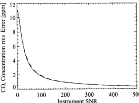
mea-surement noise is directly given by Eq.共18兲. Figure 8 shows the attainable CO2precision with respect to

the instrument SNR, expressed at the maximum at-mospheric transmittance 共tatm ⫽ 1兲. We observe a

strongly linear relation between the inverse of the CO2 relative precision and the instrument SNR.

For an instrument SNR of typically 200, the simula-tions predict a CO2 column rms error of 0.9 ppm in

the 2.0-␮m channel and 1.0 ppm in the 1.6-␮m chan-nel. Note that, for a SNR of 0, the rms error has a finite value that corresponds to the a priori uncer-tainty on the CO2concentration共set to 11 ppm兲.

C. Surface Pressure

The estimation of the CO₂column–weighted concen-tration supposes knowledge of the surface pressure

as shown by Eq. 共19兲. Mistaking the surface pres-sure by⌬P_surfinduces a relative error on the concen-tration estimates: ⌬rˆ rˆ ⫽

兰

兰

兰

column, r共P兲 can be held constant; thus, to a good approximation, ⌬rˆ rˆ ⫽ w共Psurf兲

兰

or, more simply, ⌬rˆ

rˆ ⫽ wn共Psurf兲

⌬Psurf Psurf

, (23)

where wn共P兲 is the normalized weighting function.

Accordingly, the more responsive to the lower at-mosphere the measurement is, the more it is affected by surface pressure error. In view of the weighting functions共Fig. 7兲, the impact of surface pressure un-certainty is expected to be larger in the 2.0-␮m chan-nel than in the 1.6-␮m channel 共normalized weights at the surface are 1.9 and 1.1, respectively兲.

The rms error for mean sea level pressure given by numerical weather centers is 1 hPa. This error is expected to be lower for regions of clear sky, for which valid satellite measurements are available. Thus, over the ocean, the surface pressure is known to bet-ter than 1‰ relative rms and the corresponding error in CO2-weighted concentration is better than 1‰ or

0.4 ppm.

Over land surfaces, there is an additional uncer-tainty due to the altitude of the measurement spot. The surface pressure decreases by 1 hPa共or roughly

Fig. 7. Predicted vertical weighting functions as a function of pressure 共dimensionless averaging kernels兲. The dashed and solid curves are for the 1.6- and the 2.0-␮m channels, respectively.

Fig. 8. Retrieval error of the CO2-weighted concentration as a

function of the instrumental SNR. Dashed and solid curves, the 1.6- and the 2.0-␮m channels, respectively.

1‰兲 for an increase in altitude of around 8 m. Thus the effective altitude of the spot must be known with an accuracy of 8 m. This requirement clearly ex-cludes mountainous regions for which it will not be possible to define an effective altitude to this degree of precision at the expected spatial resolution of a few kilometers. For regions with limited relief共i.e., with a standard deviation of the altitude within the mea-surement spot that is less than a few tens of meters兲, digital elevation models are available. The accuracy of these models is currently of the order of a few tens of meters and will improve dramatically within the following years with the release of the data acquired during the Shuttle Radar Topography Mission. Nevertheless, it is clear that surface topography brings an additional error source for measurements made over land surfaces. If we assume a typical error of 30 m on the pixel’s surface altitude, and are well aware that this value varies greatly with the area, it results in an additional error on the column-weighted concentration of 4‰, or 1.5 ppm overland. This error is mostly random and may decrease within the coming years with better knowledge of topogra-phy. Moreover, using a simultaneous measurement in an oxygen band, such as that envisioned for atmo-spheric scattering correction 共see Subsection 5.E兲, may significantly reduce the surface pressure impact on the concentration estimate.

D. Temperature Sensitivity

Temperature has an impact on the absorption coeffi-cients of CO2. Therefore imperfect knowledge of the

atmospheric temperature profile yields an error in the CO2concentration estimate. The inversion

pro-cedure assumes a temperature profile as provided by the reanalysis of the NWP models. Typical rms er-rors for the temperature profile are currently around 1 to 1.5 K. Note that this may decrease in the future with the constant improvement of weather forecast models and the associated assimilation procedures. These errors are slightly correlated in the vertical and therefore tend to compensate for one another statistically. Thus the assumption of a constant bias of such magnitude on the vertical profile would result in unrealistic large errors on the CO₂column estimate. Using a correlated noise generator, we simulated a field of 1000 realistic vertical profiles of temperature errors in order that their statistics match the variance– covariance matrix derived by the

60-level European Center for Medium-Range

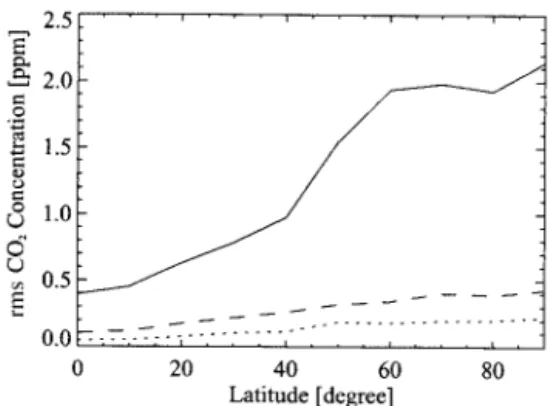
Weather Forecasts共ECMWF兲 model. Following the method described earlier, we analyzed the mean im-pact on the CO₂column estimate共Fig. 9兲. The con-centration rms errors are lower in the tropics, where the rather low temporal and spatial variabilities of the temperature profile facilitate the capture by me-teorological models. Temperature is a major source of error in the 2.0-␮m channel, but the error is very much lower in the 1.6-␮m channel 共about six times lower兲. For measurements at midlatitude 共40 deg兲, we predict typical errors of 0.3 and 1.7 ppm in the 1.6-and the 2.0-␮m channels, respectively. This large

difference is inherent to the spectroscopic parameters of the absorption lines in the selected portions of the absorption bands. The integrated absorption coeffi-cient of a line共i.e., the line intensity兲 S_iis dependent on temperature according to

Si⫽ Si

0

Q共T0兲兾Q共T兲exp关⫺c2E⬙i共1兾T

0_{⫺ 1兾T兲兴, (24)}

where E⬙_iis the energy of the lower state of the tran-sition. As shown in Fig. 10, the relative change of CO₂line intensity caused by a perturbation of tem-perature is very much a function of the lower state energy of the transition. Typically, for lines with E⬙_i below 300 cm⫺1, Si varies by less than 1% per unit

degree at characteristic atmospheric temperatures. At larger E⬙i, the percentage change increases

signif-icantly, especially over the range of stratospheric temperature 共200–270 K兲. For the principal CO2

isotope, E⬙_i lies from 464.17 to 1188.29 cm⫺1in the 2.0-␮m channel and from 2.34 to 234.08 cm⫺1in the 1.6-␮m channel. Therefore the absorption lines in the 1.6-␮m channel are significantly less sensitive to

temperature errors. Note that the percentage

changes of line intensity in Fig. 10 slightly differ from

Fig. 9. CO2-weighted concentration rms error due to uncertainty

on the temperature profile as a function of latitude in the 2.0-␮m channel共solid curve兲 and the 1.6-␮m channel 共dashed curve兲. The dotted curve shows the achievable error by use of simultaneous measurements in both bands. The simulation used 1000 synthet-ically noised temperature profiles.

Fig. 10. Relative change of CO2line intensity caused by a unit

degree perturbation of temperature as a function of temperature for various lower state energies E_{⬙. Partition sum functions used} in the computation are issued from HITRAN 2000.

those obtained by Park,35_{owing to different values of}

the CO2partition functions in the calculation.

Let us point out that the established temperature sensitivities are a direct function of the chosen spec-tral intervals. If the spectral windows were shifted or chosen wider, they would encompass absorption lines with a different range of E_i, and this would affect the overall dependences on temperature. In addition, if simultaneous measurements in both 1.6-and 2.0-␮m channels are performed, the different temperature sensitivities of the bands can be used to reduce the temperature uncertainty on the CO2

esti-mate as we now explain: Temperature-averaging

kernels of the 1.6- and the 2.0-␮m channels 共Fig. 11兲 show a clear anticorrelation. In consequence, it is expected that a given field of error in the temperature profile will affect the CO₂retrieval of the two chan-nels in a connective manner. The representation of the synthesized 1000 errors in a scatter plot共Fig. 12兲 reveals a simple linear relation共solid line兲 in the form

εCO2 1.6 _{⫽ ␣ε} CO2 2.0_{, (25)} with ␣ ⫽ ⫺0.1670, where εCO2 1.6 and εCO2 2.0 denote the CO₂retrievals in the 1.6- and 2.0-␮m channels, re-spectively.

The constraint that the retrieved CO₂must be the

same from both bands suggests the corrected esti-mate: rˆCO2⫽ rˆCO2 1.6 _{⫺ ␣rˆ} CO2 2.0 1⫺ ␣ , (26) where rˆCO2 1.6 and rˆCO2 2.0

are the retrieved CO2 values in

the 1.6- and 2.0-␮m channels, respectively. Because errors will be mostly compensated for in Eq.共26兲, the sensitivity to errors in the a priori temperature pro-file will be significantly reduced. Simulations show that, after correction, the rms errors on the CO₂ re-trieval are contained below 0.2 ppm at all latitudes 共dotted curve in Fig. 9兲.

E. Atmospheric Scattering

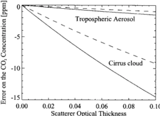
Atmospheric scattering allows photons that have not traversed the full double atmospheric path to be mea-sured. Because this light traverses less material, it is less absorbed by the CO₂and yields a lower appar-ent concappar-entration. The quantitative impact is a function of both optical properties and height, which are highly variable in space and time. Observations in the presence of thick clouds can be identified and filtered out, but undetectable scatterers, such as sub-visible cirrus, are a potential source of error that needs to be assessed. In Fig. 13 we present the er-rors associated with a boundary-layer aerosol distrib-uted around 900 hPa and a cirrus cloud distribdistrib-uted around 250 hPa as a function of optical depth. In this simulation, we assumed a nonabsorbing scat-terer and a Henyey–Greenstein36,37_{phase function.}

Aerosol optical properties are now well known thanks to considerable effort during the past decade, including research with surface Sun photometers and satellite measurements. Most aerosols show a rapid decrease of the optical thickness with the wavelength so that it is relatively minor at 1.6 and 2␮m except for specific cases such as dust storms. Moreover, aerosol layers are generally low in the atmosphere. Typically, the presence of a boundary-layer aerosol at

Fig. 11. Dimensionless temperature-averaging kernels for the 2.0-␮m channel 共solid curve兲 and the 1.6-␮m channel 共dashed curve兲.

Fig. 12. Correlation between εCO2

1.6 _{and ε} CO2

2.0_{. The calculation}

used the same field of noised temperature profiles as for Fig. 9.

Fig. 13. Retrieval error of the CO2-weighted concentration owing

to atmospheric scattering as a function of the scatterer optical thickness. We considered the case of a cirrus cloud distributed around 250 hPa and a boundary-layer aerosol distributed around 900 hPa. The simulation was made for a SZA and a VZA of 45 deg and a surface reflectance of 0.2. The dashed and solid curves are for the 1.6- and the 2.0-␮m channels, respectively.

an average height of 1 km with an optical thickness of 0.05 in the spectral range of interest above a surface of reflectance 0.2 is expected to generate an error of approximately 1.5 ppm共0.45%兲 for a SZA or VZA of 45 deg.

A similar evaluation is more difficult for thin cir-rus clouds because it requires a reliable estimate of their optical thickness. Furthermore, assuming it were possible to select observations totally free of thin cirrus clouds, we ignore whether such clear areas would represent a significant fraction. Us-ing MODIS-calibrated radiance products, we pro-cessed optical thickness histograms at 1.6 and 2.1 ␮m over the ocean 共not shown兲. Regions contami-nated by clouds or Sun glint were removed so that atmospheric scattering generates the main contri-bution to the TOA radiance. Our analysis reveals that even the apparently clearest cases over the open oceans seem to be affected by atmospheric scattering with typical optical thickness of 0.02 共after molecular scattering correction兲. These re-sults indicate that most of the clear cases may, in fact, be contaminated by thin cirrus layers with an unacceptable共over 1%兲 impact on the CO2apparent

concentration.

Fortunately, the effect of scattering by thin clouds and aerosols on the estimation of the CO2 column

amount can be largely mitigated by use of dedicated schemes. Promising techniques have been proposed to correct for this error in previous studies.16,17,38

One strategy consists of compensating for the scat-tering error by using supporting measurements in an oxygen band in addition to the CO₂ absorption band.16,17 _{Because oxygen is a well-mixed gas in the}

atmosphere and its density is mostly constant, its absorption spectrum yields a scattering vertical pro-file that may be used to correct the apparent CO2

concentration. O’Brien and Rayner16 _have

demon-strated the potential of such a method applied to high-resolution measurements at a few frequencies in the 1.61-␮m absorption band of CO2 and the

1.27-␮m absorption band of O2. The results indicate

that the proposed algorithm allows for scattering er-ror reduction to below the 0.5% level in situations with cirrus and aerosol optical thickness as large as 0.1 and 0.2, respectively. Another method, sug-gested by Aoki et al.,38_{relies on the analysis of the}

polarized radiation in the Sun-glint region. The dif-ference between the polarization rate of the surface-reflected radiation over Sun glint and that of the scattered radiation in the atmosphere is exploited to eliminate the impact of scattering by appropriately differentiating two components of the polarized light. It is found that the effect of the radiation scattered by thin clouds and aerosol on the estimation of the CO2

column amount can be reduced to below 0.1%. Sim-ilar procedures could be applied to the spectra inver-sion that is discussed here, although an evaluation of the expected accuracy would be the subject of a full paper.

F. Knowledge of Spectroscopic Parameters

The accuracy of the absorption intensity for the lines of interest is not better than several percentages 关HI-TRAN or GEISA39 共Gestion at Etude des

Informa-tions Spectroscopiques Atmosphe´riques兲 databases兴. The relative accuracy for the other parameters 共line width and sensitivity to temperature and pressure兲 is even lower. Clearly, this accuracy is not sufficient for determining the absolute abundance of CO₂. There is a strong need to better characterize the nec-essary coefficients. This can be carried out either in the laboratory or, for better compatibility with the spaceborne measurements, using a spectrometer, aiming at the Sun with a concomitant airborne profile measurement of CO₂. In view of that, it can be rea-sonably expected that the error associated with spec-troscopic parameter uncertainty will become less than 0.5%. Besides, such remaining errors will be mostly systematic, with limited impact on the surface flux estimates in that those are derived from atmo-spheric CO₂gradients rather than absolute levels.

G. Atmospheric Water Vapor

The CO2flux inversion methods, which may use

sat-ellite estimates of CO2 concentration, are based on

the dry-air volume mixing ratio. For a given dry-air volume mixing ratio, water vapor in the atmosphere increases the total air mass and therefore decreases the concentration of CO2. Atmospheric water-vapor

content and its uncertainty are very much a function of latitude and season 共linked to the temperature through the atmospheric capacity兲. In midlatitude, a typical H2O content is 10 kg m⫺2or 1‰ of the total

atmospheric mass. By use of fields from NWP mod-els, the uncertainty can be reduced to a fraction of this value. In the tropics the total water-vapor con-tent can rise to 100 kg m⫺2, and a typical uncertainty is 10 kg m⫺2 or 1‰ of the total atmospheric mass. Therefore a typical error on the conversion between the CO2 volume mixing ratio and the dry-air CO2

volume mixing ratio is between 0.1 and 1‰. This error may decrease in the future with the constant improvement of weather models and the associated assimilation procedures of satellite data.

6. Conclusions

In this paper we discuss the accuracy of CO2column

spaceborne estimates from spectroscopic measure-ments at high resolution in the 1.6- and 2-␮m absorp-tion bands by using the differential absorpabsorp-tion technique. The accuracy required to improve our knowledge of the carbon budget is on the order of 1% or 3.6 ppm. Because of this stringent requirement, many sources of error have to be considered that are neglected when a similar technique is used for other gases.

The error budget 共Table 3兲 indicates that the ob-jective is difficult to attain on individual shots. Sev-eral sources of error amount to between 1 and 2 ppm. The weighting function of the 2.0-␮m channel in-creases with pressure, which makes it more sensitive

to the boundary layer, where the concentration gra-dients are expected to be the largest and the easiest to relate to surface fluxes. This makes it better suited to the science objectives than the 1.6-␮m chan-nel. On the other hand, the 1.6-␮m channel is less sensitive to several sources of uncertainties, in par-ticular, the temperature profile and the surface pres-sure.

There are two major sources of error that need to be resolved for a useful measurement of the CO₂ from space by using the method described in this paper. One is the spectroscopic parameters. This can be resolved relatively easily from additional Sun pho-tometry measurements from surface-based instru-ments during the development of the space mission. The other one is the impact of atmospheric scattering resulting from aerosol and undetected clouds. This error can be rather large and may lead to spatial biases as the distribution of atmospheric scatterers is not uniform. Additional studies are needed to prop-erly evaluate this source of uncertainty and the ac-curacy of a correction algorithm that uses an oxygen absorption band.

The authors thank P. Couvert at Laboratoire des Sciences du Climat et de l’Environnement for provid-ing the POLDER data used for Fig. 4. Similarly, we are glad to acknowledge the assistance of F. Cheva-lier at ECMWF who provided us with the ECMWF model temperature error matrices and the correlated noise generator used for Figs. 9 and 12. This paper benefited a great deal from an extremely detailed and competent criticism by an anonymous reviewer. We are grateful for the time and effort he put into his review. This work received some support from the Centre National d’Etudes Spatiales and the Euro-pean Union funded project COCO, EVG1, CT2001-00056.

References

1. T. J. Conway, P. P. Tans, L. S. Waterman, and K. W. Thoning, “Evidence for interannual variability of the carbon cycle from the National Oceanic and Atmospheric Administration, Cli-mate Monitoring and Diagnostics Laboratory global air-sampling network,” J. Geophys. Res. 99, 22831–22855_共1994兲. 2. J. T. Houghton, Y. Ding, D. J. Griggs, M. Noguer, P. J. van der Linden, X. Dai, K. Maskell, and C. A. Johnson, eds., Climate

Change 2001: The Scientific Basis. Contribution of Working Group I to the Third Assessment Report of the Intergovernmen-tal Panel on Climate Change共IPCC兲 共Cambridge U. Press, New

York, 2001_兲.

3. I. G. Enting, C. M. Trudinger, and R. J. Francey, “A synthesis inversion of the concentration and␦13_{C of atmospheric CO}

2,”

Tellus Ser. B 47, 35–52_共1995兲.

4. P. Ciais, P. P. Tans, M. Trolier, J. W. C. White, and R. J. Francey, “A large northern-hemisphere terrestrial CO2sink

indicated by the13_C兾12_{C ratio of atmospheric CO}

2,” Science

269, 1098 –1102共1995兲.

5. P. J. Rayner, I. G. Enting, R. J. Francey, and R. Langenfelds, “Reconstructing the recent carbon cycle from atmospheric CO2,

␦13_{C and O}

2兾N2 observations,” Tellus Ser. B 51, 213–232

共1999兲.

6. P. Bousquet, P. Ciais, P. Peylin, M. Ramonet, and P. Monfray, “Inverse modeling of annual atmospheric CO2 sources and

sinks 1. Method and control inversion,” J. Geophys. Res. 104, 26161–26178_共1999兲.

7. P. Bousquet, P. Peylin, P. Ciais, M. Ramonet, and P. Monfray, “Inverse modeling of annual atmospheric CO2 sources and

sinks 2. Sensitivity study,” J. Geophys. Res. 104, 26179 – 26193共1999兲.

8. P. J. Rayner and D. M. O’Brien, “The utility of remotely sensed CO2concentration data in surface source inversions,” Geophys.

Res. Lett. 28, 175–178_共2001兲.

9. A. Chedin, S. Serrar, R. Armante, N. A. Scott, and A. Hollings-worth, “Signatures of annual and seasonal variations of CO2

and other greenhouse gases from comparisons between NOAA TOVS observations and radiation model simulations,” J. Clim.

15, 95–116_共2002兲.

10. R. J. Engelen, A. S. Denning, K. R. Gurney, and G. L. Ste-phens, “Global observations of the carbon budget: 1. Ex-pected satellite capabilities for emission spectroscopy in the Table 3. Estimate of the Various Error Sources Identified and Quantified in this Paper for the Retrieval

of CO2-Weighted-Column Concentration from Space

Error Source Assumed Uncertainty

Error_共ppm兲 2.0_␮m

Error_共ppm兲

1.6_␮m Comment

Radiometric noise SNR⫽ 200 0.9 1 Random

Temperature profile Current ECMWF error at 50° latitude 1.7 0.4 Can be improved to 0.2 ppm by using coincident measure-ment in both channels

Surface pressure Ocean: ⬍1 hPa 0.6 0.3 Random. May decrease with

new Digital Elevation Model

Land: 5 hPa 3.6 1.8 Can be corrected by addition of

an O2band

Water vapor H2O column: 1–10 kg m⫺2 0.03–0.3 0.03–0.3 Random. May improve with

NWP models Atmospheric

scatter-ing

Thin cirrus optical thickness 0.02 4 4 Can be corrected by addition of an O2band

Aerosol optical thickness 0.05 1.5 1.5

Absorption coefficient 4% 15 15 Bias. Will decrease to better

than 0.5% with laboratory measurements