Historical droughts in Mediterranean regions during the last 500 years: a data/model approach

(1)

HAL Id: hal-00330714

https://hal.archives-ouvertes.fr/hal-00330714

Submitted on 12 Sep 2006

HAL is a multi-disciplinary open access

archive for the deposit and dissemination of sci-entific research documents, whether they are pub-lished or not. The documents may come from teaching and research institutions in France or abroad, or from public or private research centers.

L’archive ouverte pluridisciplinaire HAL, est destinée au dépôt et à la diffusion de documents scientifiques de niveau recherche, publiés ou non, émanant des établissements d’enseignement et de recherche français ou étrangers, des laboratoires publics ou privés.

Historical droughts in Mediterranean regions during the

last 500 years: a data/model approach

S. Brewer, S. Alleaume, Joel Guiot, A. Nicault

To cite this version:

S. Brewer, S. Alleaume, Joel Guiot, A. Nicault. Historical droughts in Mediterranean regions during the last 500 years: a data/model approach. Climate of the Past Discussions, European Geosciences Union (EGU), 2006, 2 (5), pp.771-800. �hal-00330714�

(2)

CPD

2, 771–800, 2006

Historical Mediterranean droughts: data and

models S. Brewer et al. Title Page Abstract Introduction Conclusions References Tables Figures J I J I Back Close

Full Screen / Esc

Printer-friendly Version Interactive Discussion

Clim. Past Discuss., 2, 771–800, 2006 www.clim-past-discuss.net/2/771/2006/ © Author(s) 2006. This work is licensed under a Creative Commons License.

Climate of the Past Discussions

Climate of the Past Discussions is the access reviewed discussion forum of Climate of the Past

Historical droughts in Mediterranean

regions during the last 500 years: a

data/model approach

S. Brewer1, S. Alleaume1, J. Guiot1, and A. Nicault2

1

CEREGE, CNRS/Universit ´e Paul C ´ezanne UMR 6635, BP 80, 13545 Aix-en-Provence cedex, France

2

Centre d’Etudes Nordiques, Universit ´e Laval, Ste Foy, Qu ´ebec GlK7P4, Canada

Received: 31 March 2006 – Accepted: 4 September 2006 – Published: 12 September 2006 Correspondence to: S. Brewer (brewer@cerege.fr)

(3)

CPD

2, 771–800, 2006

Full Screen / Esc

Abstract

We present here a new method for comparing the output of General Circulation Models (GCMs) with proxy-based reconstructions, using time series of reconstructed and sim-ulated climate parameters. The method uses k-means clustering to allow comparison between different periods that have similar spatial patterns, and a fuzzy logic-based 5

distance measure in order to take reconstruction errors into account. The method has been used to test two coupled ocean-atmosphere GCMs over the Mediterranean region for the last 500 years, using an index of drought stress, the Palmer Drought Severity Index. The results showed that, whilst no model was able to exactly simulate the reconstructed changes, all simulations were an improvement over using the mean 10

climate. Further, a good match was found after 1650 with a model run that took into account changes in volcanic forcing, solar irradiance, and greenhouse gases. A more detailed investigation of the output of this model showed the existence of a set of at-mospheric circulation patterns linked to the patterns of drought stress: 1) a blocking pattern over northern Europe linked to dry conditions in the south prior to the Little Ice 15

Age (LIA) and during the 20th century; 2) a NAO-positive like pattern with increased westerlies during the LIA; 3) a NAO-negative like period shown in the model prior to the LIA, but that occurs most frequently in the data during this period. The results of the comparison emphasise the importance of the inclusion of the various forcings in the models and help to understand the atmospheric changes connected to reconstructed 20

climate changes.

1 Introduction

Climate models built to predict future climate change under changing environmental conditions, such as atmospheric composition, must be tested against available climatic series. Available instrumental datasets only cover a few decades and the climatic vari-25

ability of these records are often inferior to simulated future changes. Recently, clima-772

(4)

CPD

2, 771–800, 2006

Full Screen / Esc

tologists have started to test their models by simulating climates that are much different from the recent past. This has been the main goal of the Paleoclimate Modeling Inter-comparison Project (PMIP) (Joussaume and Taylor,1995). The 6000 yr. BP climate has been chosen as a key period for PMIP (Harrison et al.,1998) because it is a simple modelling experiment with a clear forcing (maximum summer insolation and minimum 5

winter insolation). However, tests of the simulated variability for this period are lim-ited by the fact that the majority of the available data have a relatively low resolution (decadal at best). In contrast, a large number of climate records with annual resolution are available for the recent past (e.g. the last millennium), notably tree-ring proxies and written historical documents. As the internal climate variability generated by the exter-10

nal forcings of this period is relatively small, coupled ocean- atmosphere models are required to accurately represent the variability of the past few centuries.

The last millennium is of particular interest as, in addition to the available proxy data, it contains two contrasted periods: the Little Ice Age (LIA), which lasted from approxi-mately 1650 to 1850, characterised by cold records in written historical sources (Lamb, 15

1977;Bradley and Jones,1992) and the Medieval Warm Period (MWP), approximately

1000–1200, characterised by a warm climate under which, notably, Vikings were able to settle on Greenland. There is a great deal of debate concerning the timing of these periods because, unlike the recent warming, they are not global in nature (Hughes and

Diaz,1994;Crowley and Lowery,2000). Climate model simulations have been used to 20

study the characteristics of these periods as well as attempting to gain insight into the mechanisms that caused these variations (Cusbach et al.,1997;Crowley,2000;

Shin-dell et al., 2001;Goosse and Renssen,2004). As many of the climatic mechanisms that will play a significant role in future changes (in addition to greenhouse gases) are important over the last millennium, data-model comparisons for this period provide an 25

opportunity to investigate how robustly these mechanisms are taken into account in the model and to identify possible improvements (Jones et al.,1998).

Due to high computer-time requirements, only a few simulations spanning at least the last 500 years have been published to date (Cusbach et al.,1997;Rind et al.,1999;

(5)

CPD

2, 771–800, 2006

Full Screen / Esc

Waple et al.,2002; Gonzalez-Rouco et al.,2003; Widmann and Tett,2003). The

cli-mate may be more easily simulated over several centuries by intermediate complexity models, but at the expense of spatial resolution. Goosse et al.(2005) have compared 25 simulations for the last millenium using the ECBILT-CLIO model and compared them to temperature reconstructions from proxy data (Villalba,1990;Briffa et al.,1992;Mann

5

et al.,1999;Briffa et al.,2001;Luterbacher et al.,2004). They concluded that MPW and LIA were hemispheric-scale phenomena, but that, during these periods, synchronous peaks in temperature at different locations were unlikely.

Simulations of the last millenium have been used, to not only better understand the models, but also the proxy based reconstructions. Zorita et al. (2003) used pseudo-10

proxies derived from temperature simulations to assess the quality of the reconstruc-tion, by investigating biases in the proxy network.von Storch et al.(2004) have further advanced this idea, by testing the effect of the fact that a proxy is an imperfect record of a given climatic parameter.

The majority of model-data comparisons using paleoclimate data (Liao et al.,1994; 15

Texier et al., 1997; Masson et al., 1998; Prentice et al., 1998) have been limited to

simple maps, time-series or data comparison in a few regions, and only simple statis-tics have been used. Frequently, error bars as well on the proxy data reconstructions and model simulations have not been taken into account. The implementation of a quantitative comparison method that is flexible enough to catch the main features of 20

the mechanisms involved is problematic (Airey and Hulme,1995). Ideally, we would like the goodness-of-fit measure to take into account situations when a model correctly simulates a particular structure in the data but with a shift in location. In this case, the fit between the model and data should be better than situations when the structure is not simulated at all. An example would be the simulation of an enhanced monsoon, but 25

not exactly the right place versus no simulated enhancement in the monsoon. In the first case (structure present, but geographically shifted), tests based on point-by-point similarities are likely to be disappointingly small. Finally, the method must also be able to take into account the uncertainties of both the proxy-derived variables and model

(6)

CPD

2, 771–800, 2006

Full Screen / Esc

outputs. In order to address the problem of uncertainties, Guiot et al. (1999) have developed a fuzzy logic approach for data-model comparisons where the compared quantities are not defined by a simple number but by a number with a membership function, which takes into account the error bars of the reconstructions and therefore allows some flexibility in the reconstruction.Bonfils et al.(2004) have further improved 5

the method by replacing the pixel-to- pixel comparison by an approach based on clus-ters, allowing comparisons to be made between spatial patterns of climate change rather than individual points. In this paper, we propose an adaptation of this method for spatio-temporal data, rather than static time-slice data.

In addition to spatial variability, coupled models simulate the temporal variability of 10

climate, which adds an additional degree of complexity. The method we propose works in several steps. The first step is to detect the major geographical patterns in the validation data by cluster analysis and to associate a given pattern to each year. A given year is then represented by a dominant pattern (plus a measure of resemblance) and not by a distribution map. We assign the same pattern to each simulation year. 15

The final comparison between data and model will be done on the basis of the centroid and extent of the clusters in the gridpoint space. This approach takes into account the spatial and temporal characteristics of the studied data without doing a strict point-to-point and time-to-time comparison.

2 Data

20

The study area used is the Mediterranean region in the spatial grid from 30◦N to 50◦N and from 10◦W to 50◦E.

2.1 Instrumental and proxy data

Climate reconstructions of the Mediterranean region based on tree-rings are compli-cated by the fact the trees respond to different climate parameters of seasonalities in 25

(7)

CPD

2, 771–800, 2006

Full Screen / Esc

different parts of the area. We have chosen to use the Palmer Drought Severity Index (PDSI) (Palmer,1965), a widely used indicator of drought conditions, which presents a number of advantages over seasonal temperature or precipitation values. The PDSI integrates both temperature and precipitation and uses a supply and demand model to estimate how the soil moisture availability differs from normal conditions. For any given 5

month, the index takes into account the value of the preceding month, and will therefore reflect recent conditions for a location. The index is calculated relative to the climatol-ogy of the location and the value of the index and the severity of the drought or wet spell is relative to the typical climate variation of the location. A dry period will therefore be considered as more severe in an area where the typical variation in climate is small. 10

The value of the index obtained and the severity of the drought are therefore compara-ble between locations that may have quite different amounts and seasonal distribution of precipitation. The index ranges between negative values for dry conditions and pos-itive values for wet conditions. Values less than −4 or greater than+4 are indicative of extreme drought or wet spells, respectively.

15

The index is calculated relative to the climatology of the location and the value of the index and the severity of the drought or wet spell is relative to the typical climate variation of the location. A dry period will therefore be considered as more severe in an area where the typical variation in climate is small. The value of the index obtained and the severity of the drought are therefore comparable between locations that may 20

have quite different amounts and seasonal distribution of precipitation.

We have used the self-calibrated PDSI (Wells et al., 2004), calculated using time series of temperature and precipitation and estimations of the Available Water Content (AWC) of the soil. For climate data, we have used the 0.5◦ gridded climate dataset obtained from the Climatic Research Unit (CRU) (Mitchell et al.,2004) and AWC esti-25

mations from the “Global Soil Types, 1-Degree Grid” (Zobler,1999).

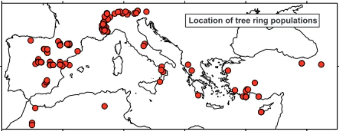
The tree-ring dataset was comprised of 136 sites distributed across the Mediter-ranean basin (Fig. 1), taken from the DENDRODB Relational European tree-ring database (http://servpal.cerege.fr/webdbdendro/). Only series longer than 300 years

(8)

CPD

2, 771–800, 2006

Full Screen / Esc

(i.e. starting before 1700) were retained. The tree-ring parameters used in this study were the total ring width (RW), the final (or late) width (LW) and the maximal den-sity (MD), as these are generally related to summer drought conditions. The resulting dataset contained 165 series: 122 RW, 21 LW and 22 MD.

A transfer function was calibrated based on these proxy data using an analogue 5

technique combined with an artificial neural network technique (Nicault et al., 20061), providing a reconstruction of the summer PDSI for the last 500 years (1500–2000) over the Mediterranean Basin on a 2.5◦ grid.

The skill of the reconstruction was tested seperately for different periods, to take into account the reduction in the number of proxies in earlier periods. The mean calibration 10

correlation coefficient varied between 0.756 and 0.88, and the mean verification corre-lation coefficient varied between 0.635 and 0.885. A bootstrap test on the calibration period showed gave an average calibration R2 of 0.732, and a verification R2 of 0.489.

2.2 Model simulations

The simulated climate data were taken from the SO&P project, and included two cou-15

pled climate models: HadCM3 (the United Kingdom Meteorological Office Hadley Centre’s 3rd coupled ocean-atmosphere model (Gordon et al., 2000) and ECHO-G (the German climate community’s ECHAM4/HOPE coupled ocean- atmosphere model

(Legutke and Voss,1999). The spatial resolution of the HadCM3 model is 3.75×2.5◦,

with 70 pixels considered as land in the study area. The horizontal resolution of the 20

ECHO-G model is T30, with 42 pixels considered as land in the study area.

Five simulations were available as results of the SO&P project (http://www.cru.uea.

ac.uk/projects/soap/):

1. HadCM3 control simulation: 1000-year simulation with constant external forcing. The full simulation is much longer than this, but 1000 years are available for use 25

1

Nicault, A., Alleaume, S., Brewer, S., and Guiot, J.: Mediteranean drought fluctuation during the last 650 years based on tree-ring data, Clim. Dyn., submitted, 2006.

(9)

CPD

2, 771–800, 2006

Full Screen / Esc

in SO&P.

2. HadCM3 natural forcings simulation (“Natural forcings”): 1492–1999 with pre-scribed changes in volcanic forcing, solar irradiance and orbital forcing, while an-thropogenic forcing factors were fixed at estimated pre-industrial values. Only the period 1500–1999 was used, due to spin up trends prior to 1500.

5

3. HadCM3 all forcings simulation (“All forcings”): 1750–1999 with prescribed changes in volcanic forcing, solar irradiance, orbital forcing, greenhouse gases, tropospheric sulphate aerosol, stratospheric ozone and land-use/land-cover. 4. ECHO-G control simulation: 1000-year simulation with constant external forcing

(Zorita et al.,2003).

10

5. ECHO-G all forcings simulation (“Erik-the-Red”): 901–1990 with prescribed changes in volcanic forcing, solar irradiance, and greenhouse gases. This run contains a significant drift in the early part of the run. Only the period 1500–1990 was retained for use in the comparison.

3 Method and results

15

The PDSI was calculated for the models using the same technique as for the recon-structions. We used monthly temperature and precipitation series expressed in re-spectively ◦C and mm/month, together with soil data from (Zobler,1999) upscaled to the resolution of the model by taking the closest soil gridpoint. The average summer PDSI for the study for each of the five simulations is shown in Fig.2, together with the 20

average proxy-based reconstructed PDSI. Simulations performed with natural forcings do not show any significant trend over the last five centuries and the 20th century is rather humid. When greenhouse gases forcing are introduced (all-forcings), the simu-lated PDSI becomes dry in the 20th century in both models. This drying starts early in the 20th century in ECHO-G and in the mid to late 20th century in HadCM3. A visual 25

(10)

CPD

2, 771–800, 2006

Full Screen / Esc

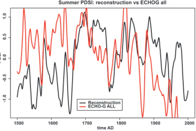
comparison of the reconstruction with simulations shows that, prior to the 20th century, the output of ECHO-all is similar to the reconstruction. Peaks of moisture are found in both curves during the 1880s, around 1810 and around 1700, whilst drier periods are found in the mid 19th century, last part of 18th century and mid 17th century. For the period where ECHO-all and the reconstruction are in closest agreement (Fig.3), 5

i.e. 1665–1890: the correlation between the smoothed series reaches 0.52. We were unable to find good correlations with the HadCM3 model runs.

3.1 Data upscaling

The spatial resolution of the model and proxy PDSI are different, and the model simu-lations would normally be downscaled to the resolution of the proxies. However, as a 10

large number of pixels are coastal, downscaling produces a large number of gridpoints interpolated from model off-shore pixels. We have therefore upscaled the proxy data to the resolution of the two models, by averaging the reconstructed PDSI around the model pixel centre, with reconstructed data pixels being attributed to the closest model pixel. The subsequent comparisons are made over the time period common to both 15

data and model simulations: 1500–1989.

3.2 k-mean cluster analysis on reconstructed PDSI and cluster assignment to models

The goal of this part of the analysis is to identify the major geographical patterns in the data, for subsequent comparison with the model. The matrix of reconstructed PDSI values is now considered as a set of 490 vectors, each representing a year between 20

1500 and 1989) and composed of m variables (one per model gridpoint). We then use the k-means algorithm (Hartigan and Wong, 1979) to group together these vectors according to their similarities. The aim here is to obtain groups of years in which the spatial pattern of the PDSI was similar. The k groups are a priori unknown: the optimum number of groups is therefore chosen by maximizing the ratio of inter-group 25

variance to intra-group variance. Five groups were selected for this dataset. 779

(11)

CPD

2, 771–800, 2006

Full Screen / Esc

In this analysis, the yearly vectors are projected into a multi-dimensional space, de-fined by a set of axes, each representing possible PDSI values at a grid point. An initial set of k years is randomly chosen as the cluster centroids and the remaining data points are assigned to the closest vector. The new k centroids are then calculated for each of these clusters. Each data point is subsequently reassigned to the closest 5

centroid and a new set of groups is obtained. This is repeated until no further reassign-ment of the data points takes place, at which point the clusters are considered stable and the process ends. As the assignation of years to particular clusters may depend on the choice of the initial centroids, we tested the stability of the clusters by repeating the clustering several times with different initial centroids, and visually checking that 10

the groups of years making up each cluster remained stable. Each cluster may now be represented by its centroid and its extent on each axis (PDSI values for each grid point). However, the centroid and extents of each cluster do not necessarily correspond to any given year. We therefore assign the year with the most similar spatial pattern to the centroid and extent. This is done by applying a principal component analysis 15

(PCA) to each cluster, sorting along the first PC axis and selecting the 5th, 50th and 95th yearly vectors. As we wish to take into account the uncertainties in the recon-struction, we adjust the upper and lower extents of each cluster by the reconstruction error. For example, if the year corresponding to the lower extent of cluster 1 was found to be 1881, then the lower extent value for any grid point will be the 1881 PDSI value 20

less the reconstruction error.

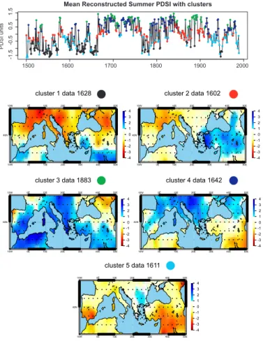
Figure 4presents the spatial pattern and temporal pattern of summer PDSI values for the region. The time series shows, for each year, the average summer PDSI value for the whole studied region and the assigned cluster. The maps show the geographical pattern of PDSI values for the five clusters, with each cluster represented by its median 25

year. The most humid clusters – cluster 3 (blue) and cluster 4 (green) - are represented by year 1642 and 1883 and dominate between 1650 and 1900, corresponding approx-imately to the LAI. Cluster 1 (black, year 1628) and cluster 5 (cyan, year 1611) show generally dry conditions. The extreme south remains humid in cluster 1, however, the

(12)

CPD

2, 771–800, 2006

Full Screen / Esc

reliability of reconstructed values in this region is poor, due to a low number of tree sites. These two patterns dominate before 1650 and during the 20th century. Cluster 2 (red), represented by year 1602, is clearly a west-east gradient and occurs throughout the entire period, notably during the mid to late 1800s.

The model output is now transformed to be comparable with the clusters obtained in 5

the previous step; this is done by assigning each simulated year to the cluster for the equivalent year in the reconstructed PDSI series. In order to obtain the centroid and extent of the simulated clusters, as before, we apply a PCA to each cluster of simulated years, sort along the first PC, then select the 5th, 50th and 95th percentiles. No error bar is available here for each simulated year.

10

At this stage, we have two arrays (one for reconstructed data and one for simula-tions), which give the centroid and extent of each of cluster in PDSI values for each grid point. For example, a given grid point may have low PDSI values for cluster 1, high for cluster 4, intermediate for cluster 5 and so on. The extents give an idea of how well constrained each cluster is. Both arrays have the same number of columns, 15

so a comparison may be made by calculating the distance between the simulated and reconstructed clusters. To take into account the variability around the centroids of the clusters and the error bars on the reconstructions, we use a fuzzy distance called the Hagaman distance (Bardossy and Duckstein,1995).

3.3 Hagaman distance between model and reconstructed data 20

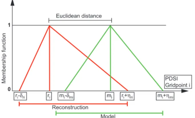
For each gridpoint i , we calculate the Hagaman distance between each reconstructed PDSI cluster R and each simulated cluster M (Fig.5). The projection of cluster A on gridpoint i can be considered as a triangular fuzzy number (r_i, r_i−δ_ri, r_i+η_ri) where r_i is the position of the triangle apex, i.e. the value with membership 1, r_i−δ_ri defines the lowest possible value, i.e. with a membership 0 and r_i+η_ri defines the highest 25

possible value with a membership, also equal to 0. We define an equivalent triangular fuzzy number for cluster M (m_i, m_i−δ_mi, m_i+η_mi). The Hagaman squared distance

(13)

CPD

2, 771–800, 2006

Full Screen / Esc

between R and M projected on gridpoint i is then:

D_i2(R, M)= (r_i− m_i)2− (1) 1 3(ri − mi)[(δri− δmi) − (ηri − ηmi)]+ 1 12[(δri − δmi) 2_{− (η} ri− ηmi)2]

Finally the total distance between R and M is the sum of the gridpoint distances: 5 D2(R, M)= 1 ms ms X i=1 D_i2(R, M) (2)

For each model, we calculate a matrix of the Hagaman distances for each cluster with the reconstructed PDSI data (Table 1). We expect that the lowest values will be found along the main diagonal, i.e. that cluster n in the model will be the most similar to cluster n in the reconstruction, but this is rarely the case. A maximum of two clusters 10

are well assigned by the models. The results are summarized in the last column of the table, which indicates, for each model cluster, the average minimum distance and the average distance along the diagonal, i.e. when the clusters correspond. ECHO-G models are generally slightly closer to the reconstructions, and the ECHO-G run with all forcings have the smallest expected distance, confirming the visual comparison of the 15

PDSI time series (Fig.3). Notably, the fit for both models increases as the complexity of the forcings used increases.

A second simple test is to consider if the simulated PDSI is closer to reconstructed values than using an equivalent length time series of mean climate values. As the PDSI is normalized by the “normal” climate of each gridpoint (equivalent to the mean 20

climatology), the variance may be considered as the mean Euclidian distance between the run and the climatology. The mean variance of each run is given in Table 2: values vary between 4.9 and 5.9 (more than the double the data variance: 2.01). In all cases, the simulations are better than the climatology.

(14)

CPD

2, 771–800, 2006

Full Screen / Esc

4 Discussion

The main modes of summer PDSI spatial distribution in the Mediterranean region have been studied by using a k-mean cluster technique, giving five clusters. We have shown that two modes are dominant during the LIA, both indicating that this period was gen-erally wet in this region. Prior to 1650, the climate was dryer, in agreement with in-5

strumental records of precipitation in Barcelona (winter and spring) (Barriendos and

Rodrigo,2005) and reconstructed precipitation in Morocco (Till and Guiot,1990). The general evolution of this mean curve is also in agreement with a reconstruction of win-ter precipitation for approximately the same region (Pauling et al.,2006), i.e. dry before 1650 and during the 20th century.

10

The comparison of summer PDSI with precipitation and/or temperature is not straightforward, as this index integrates both parameters, and is influenced by the re-cent climate history of the location, by taking account of the soil reservoir. However, this comparison indicates that the long-term variations are realistic enough to use these values in a comparison with model simulations (see also Nicault et al., 20061). The 15

resemblance between the simulated and reconstructed PDSI series were assessed using the Hagaman distance. The test performed here based on the distance between reconstructed and simulated geographical patterns of PDSI values, assessed by the Hagaman distance shows that the models are generally better able to simulate past cli-mates than just using the the modern climatology. The “all-forcing” simulated summer 20

PDSI of model ECHO-G was most similar to the reconstruction.

Luterbacher (2006) have carried out a visual comparison between the

reconstruc-tion of Mediterranean winter temperature and land precipitareconstruc-tion and the ECHO-G and HadCM3 simulations. The range of variability reproduced by the climate models for the period 1500–1990 was found to be only slightly larger than that of the reconstructions. 25

They concluded that a more thorough study was required, taking into account changes in the atmospheric circulation in both climate reconstructions and model simulations. We now attempt to further this general approach by an analysis of the spatial patterns

(15)

CPD

2, 771–800, 2006

Full Screen / Esc

obtained, interpreted using the atmospheric circulation as simulated by the ECHO-G all forcing run.

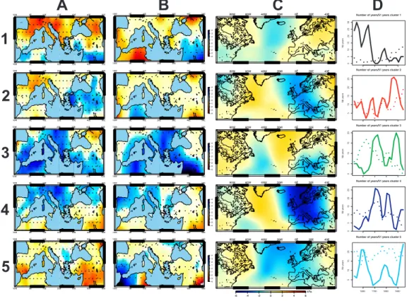
Figure6 shows a comparison of the tree-ring based PDSI reconstructions together with the model PDSI and model sea-level pressure for the equivalent years. The spatial distribution of the summer PDSI reconstructed from tree-rings is shown in column A: 5

each cluster is represented by the centroid year. The spatial distribution simulated by the model is shown in column B. In order to get the best representation of the model fields and to avoid any bias by outliers, we have selected years that belong to the same cluster in the model and the data, then taken the average of the three years closest to the data centroid. The results confirm the opposition between the driest (cluster 1) 10

and the wettest cluster (cluster 3). Cluster 4 is wet across Europe and dry over Africa and the Near East. In the model, cluster 5 shows normal conditions across the rest of the region and is humid over the southwest. This cluster is dry in the reconstructions, suggesting that this feature is not captured by the data. In contrast, cluster 1 is wet over the southwest in the data map but not in the model map. Cluster 2 appears to be 15

poorly defined in the data, as the wet pole is located over southeast, whereas in the model, it is over North Africa.

These results may be interpreted by reference to maps of sea-level pressure (SLP) fields. The patterns of summer PDSI in the Mediterranean region are mainly influenced by the period during which the majority of the precipitation falls, i.e. December of the 20

previous year to May of the current year. In addition, this corresponds to the season where the atmospheric circulation is dominated by the North Atlantic Oscillation (NAO), defined as the SLP difference between the Azores Island highs and Iceland lows (

Hur-rell, 1995). Column C of Fig. 6 shows the average SLP anomaly for the same three years representing each model cluster in comparison to the reference period 1960– 25

1989. The pressure fields are taken from the ECHO-G all forcing run and can be directly compared to the simulated PDSI maps. The clusters corresponding to specific modes of atmospheric circulation are finally represented as frequencies in the final col-umn (D), i.e. number of years per 51-year periods where the cluster is dominant for

(16)

CPD

2, 771–800, 2006

Full Screen / Esc

data and for simulations.

The dry cluster 1 is characterized by a higher than normal SLP across most of Eu-rope. The wetter conditions in the southeast can be explained by a lower SLP in this region. Higher SLP over Europe are typical of a blocking situation where anticyclonic conditions in the north force zonal circulation and thus rain to the south. This mode is 5

dominant in the reconstructions prior to 1680 and subsequently almost absent, whilst the model is not able to simulate it. Increased occurrences in the twentieth century indicate that this mode is related to global warming, implying a dryer Mediterranean region. According toLuterbacher et al. (2002), the year 1573, which belongs to this cluster, was exceptionally cold in winter. Their SLP reconstructions show high pressure 10

from Iceland to the British Isles and Central Europe and normal SLP over the Mediter-ranean region. The high pressures are correctly simulated by ECHO-G, but the low Mediterranean SLP is restricted to the east of the basin. The year 1772 is also typical of this cluster, and is considered as very warm by Luterbacher and Xoplaki (2003): their winter SLP reconstruction shows low pressure conditions over Europe, which dis-15

agrees with our results (column C). The aridity of Mediterranean region reconstructed here may therefore related to an abnormally warm and dry spring and summer, rather than winter conditions.

Cluster 2 is characterized by a lower than normal SLP in a band from Iceland to Turkey and high pressures over northeast Europe and Morocco. The difference be-20

tween the Azores highs and Iceland lows is greater than normal, resembling a positive NAO year, with the exception that SLP over the central and eastern Mediterranean re-gion are lower than might be expected (Yiou and Nogaj,2004). Under this atmospheric configuration, only the southern part of our region should be dry, not the north, which should be under the influence of increased zonal flow. This mode is dominant in the 25

reconstructions after 1850 and is correctly simulated by the model before 1800. The increase in the 20th century also suggests that, as with cluster 1, it is connected the global warming during this period.

Cluster 3 is characterized by low SLP anomalies over the Mediterranean region and 785

(17)

CPD

2, 771–800, 2006

Full Screen / Esc

high anomalies on North Atlantic Ocean and Northern Europe. This conditions re-semble a negative NAO period with a weakened zonal atmospheric circulation over Northern Europe and reinforced precipitation in the Mediterranean region (Yiou and

Nogaj, 2004). This mode is dominant in the data during the Little Ice Age (LIA) be-tween 1700 and 1900, but is more frequent in the period prior to the LIA in the model. 5

In this case, the model simulations are in better agreement with the reconstructions of Luterbacher et al. (2002) than our reconstruction. Cluster 3 includes the year 1891, characterized by a cold winter, especially in southern Europe. These conditions can be explained by low pressures in the Mediterranean region and high pressures over North Atlantic Ocean, inducing a easterly flow across the Mediterranean (Luterbacher

10

and Xoplaki,2003). This pattern is correctly simulated by ECHO-G (Fig.6: map C2). Another cold year is 1740, during which a stationary anticyclone was centered over the British Isles, resulting in easterly and northeasterly winds across western Europe

(Luterbacher et al.,2002). This year is also correctly simulated.

Cluster 4 is characterized by low pressures over western Europe and high pressures 15

over the North Atlantic Ocean. This SLP pattern does not appear to strongly influence the humidity in southern Europe wetness. This pattern resembles a positive NAO, with an enhancement of atmospheric circulation over northern Europe with corresponding higher precipitation (Yiou and Nogaj,2004), seen in Fig.6: map B4. This mode occurs frequently during the LIA in both the reconstructed PDSI and in the model PDSI, and 20

was also shown byLuterbacher et al.(2002). The winter of 1864, a year representa-tive of this cluster, was markedly wet in the Mediterranean region due to lower pres-sure in the Mediterranean and higher prespres-sure over Scandinavia and Western Russia

(Luterbacher and Xoplaki,2003). Moist air from the west and northwest was advected

towards southwest, increasing precipitation. This is not confirmed by spatial pattern of 25

this cluster, which is relatively dry in the south. However, this may result from a warm and dry following summer.

Cluster 5 is characterized by slightly lower SLP over western Europe and Atlantic Ocean and slightly higher SLP over northeast Europe. This cannot be related to a

(18)

CPD

2, 771–800, 2006

Full Screen / Esc

clear pattern of atmospheric circulation. This mode dominates before and after the LIA in the data, but is important throughout the whole period in the model simulation. The low value of the anomalies for this cluster suggest that it represents periods of little change, and will be assigned when no other cluster, with more significant changes, is better.

5

The comparison presented here emphasizes a number of climatic features that the model is able to simulate correctly: (1) the blocking situation over Europe that induces low winter precipitation corresponds to the reconstructions of some typical years. How-ever, the more humid conditions simulated prior to 1650 and the dry conditions sim-ulated after 1900 are in conflict with the data; (2) the negative NAO with enhanced 10

precipitation in the Mediterranean region corresponds well to data. This mode is, how-ever, exaggerated prior to 1650, due to the tendency of the model to be too humid during his period; (3) the dominant NAO-positive like pattern situation during the LIA, with an enhancement of humid westerlies across northern Europe agrees well with the data.

15

5 Conclusions

1. The adaptation of the method of model-data comparison to time series of simu-lated climate has allowed us to test time-series of GCM output against reconstruc-tions of PDSI for the Mediterranean region for the last 500 years in a quantitative way. The use of cluster analysis has allowed the identification of the main patterns 20

of changes in humidity and the temporal occurrence of these patterns.

2. Whilst no good agreement was found between the majority of the available climate runs and the reconstructed PDSI, all simulations offer an improvement over the mean climatology.

3. The all forcing run of ECHO-G was shown to agree well with the reconstructed 25

index over the period 1665–1890. The simulated drying in the twentieth century 787

(19)

CPD

2, 771–800, 2006

Full Screen / Esc

is, however, greater than any reconstructed changes.

4. Examination of the corresponding SLP patterns for ECHO-G has allowed an in-terpretation of the PDSI clusters in terms of changes in atmospheric circulation. These include (1) a blocking situation to the north with corresponding dry winters; (2) increased winter precipitation in the south corresponding to the NAO-negative 5

like pattern of SLP; (3) a NAO-positive pattern, with a wetter northern Europe, frequent during the LIA.

Acknowledgements. This work is contribution to the EU-project SO&P: simulations,

observa-tions and palaeoclimatic data (EVK2-CT-2002-0160SOAP).

References

10

Airey, M. and Hulme, M.: Evaluating climate model simulations of precipitation : Methods,

problems and performance., Progress in Physical Geography, 19, 427–448, 1995. 774

Bardossy, A. and Duckstein, L.: Fuzzy Rule-Based Modelling with Applications to Geophysical,

Biological, and Engineering Systems, CRC Press, Boca Raton, Florida, 1995. 781

Barriendos, M. and Rodrigo, F.: Seasonal rainfall variability in the Iberian peninsula from the

15

16th century: preliminary results from historical documentary sources, Geophys. Res. Abstr.,

7, 3533, 2005. 783

Bonfils, C., de Noblet-Ducoudre, N., Guiot, J., and Bartlein, P.: Some mechanisms of mid-Holocene climate change in Europe, inferred from comparing PMIP models to data, Clim.

Dyn., 23, 79–98, 2004. 775

20

Bradley, R. and Jones, P.: Climate since A.D. 1500, Routledge, London, 679 pp., 1992. 773

Briffa, K., Jones, P., Bartholin, T., Eckstein, D., Schweingruber, F., Karlen, W., Zetterberg, P.,

and Eroren, M.: Fennoscandian summers from AD 500: temperature changes on short and

long timescales., Clim. Dyn., 7, 111–119, 1992. 774

Briffa, K., Osborn, T., Schweingruber, F., Harris, I., Jones, P., Shiyatov, S., and Vaganov, E.:

25

Low-frequency temperature variations from a northern tree ring density., J. Geophys. Res.,

106, 2929–2941, 2001. 774

Crowley, T.: Causes of climate change over the past 1000 years., Science, 289, 270–277,

2000. 773

(20)

CPD

2, 771–800, 2006

Full Screen / Esc

Printer-friendly Version Interactive Discussion Crowley, T. and Lowery, T.: How warm was the Medieval Warm Period?, Ambio, 29, 51–54,

2000. 773

Cusbach, U., Voss, R., Hegerl, G., Waszkewitz, J., and Crowley, T.: Simulation of the influ-ence of solar radiation variations on the global climate with an ocean-atmosphere general

circulation model, Clim. Dyn., 13, 757–767, 1997. 773

5

Gonzalez-Rouco, F., von Storch, H., and Zorita, E.: Deep soil temperature as proxy for surface air-temperature in a coupled model simulation of the last thousand years, Geophys. Res.

Lett., 30, 2116, doi:10.1029/2003GL018264, 2003. 774

Goosse, H. and Renssen, H.: Exciting natural modes of variability by solar and volcanic forcing:

idealized and realistic experiments, Clim. Dyn., 21, 153–163, 2004. 773

10

Goosse, H., Renssen, H., Timmermann, A., and Bradley, R.: Internal and forced climate vari-ability during the last millennium: a model-data comparison using ensemble simulations.,

Quat. Sci. Rev., 24, 1345–1360, 2005. 774

Gordon, C., Cooper, C., Senior, C., Banks, H., Gregory, J., Johns, T., Mitchell, J., and Wood, R.: The simulation of SST, sea ice extents and ocean heat transports in a version of the Hadley

15

Centre coupled model without flux adjustments, Clim. Dyn., 16, 147–168, 2000. 777

Guiot, J., Boreux, J. J., Braconnot, P., Torre, F., and PMIP participating groups: Data-model

comparisons using fuzzy logic in palaeoclimatology, Clim. Dyn., 15, 569–581, 1999. 775

Harrison, S., Jolly, D., Laarif, F., Abe-Ouchi, A., Herterich, K., Hewitt, C., Joussaume, S., Kutzbach, J., Mitchell, J., De Noblet, N., and Valdes, P.: Intercomparison of simulated global

20

vegetation distributions in response to 6kyr BP orbital forcing., J. Climate, 11, 2721–2742,

1998. 773

Hartigan, J. and Wong, M.: A K-means clustering algorithm, Appl. Statist., 28, 100–108, 1979.

779

Hughes, M. and Diaz, H.: Was there a “Medieval Warm Period”, and if so, where and when?,

25

Climatic Change, 26, 109–142, 1994. 773

Hurrell, J.: Decadal trends in the North Atlantic oscillation: Regional temperatures and

precipi-tation., Science, 269, 676–679, 1995. 784

Jones, P., Briffa, K., Barnett, T., and Tett, S.: High- resolution palaeoclimatic records for the last millennium: interpretation, integration and comparison with General Circulation Model

30

control-run temperatures., The Holocene, 8, 455–471, 1998. 773

Joussaume, S. and Taylor, K.: Status of the Paleoclimate Modeling Intercomparison Project (PMIP), in: Proc. 1st Int. AMIP Scientific conference, WRCP Report, vol. 92, pp. 425–430,

(21)

CPD

2, 771–800, 2006

Full Screen / Esc

Monterey, CA, 1995. 773

Lamb, H. H.: Climate: present, past and future, Methuen, London, 825 pp., 1977. 773

Legutke, S. and Voss, R.: ECHO-G, the Hamburg atmosphere-ocean coupled circulation

model, DKRZ technical report 18, DKRZ, Hamburg, 1999. 777

Liao, X., Street-Perrott, F., and Mitchell, J.: GCM experiments with different cloud

parame-5

terization: comparisons with palaeoclimatic reconstructions for 6000 years BP, Data and

Modelling, 1, 99–123, 1994. 774

Luterbacher, J., Xoplaki, E., Casty, C., Wanner, H., Pauling, A., Kuttel, M., Rutishauser, Bronni-mann, S., Fischer, E., FleitBronni-mann, D., Gonzalez-Rouco, F. J., Garcia-Herrera, R., Barriendos, M., Rodrigo, F., Gonzalez-Hidalgo, J. C., Angel Saz, M., Gimeno, L., Ribera, P., Brunet, M.,

10

Paeth, H., Rimbu, N., Felis, T., Jacobeit, J., Dunkeloh, A., Zorita, E., Guiot, J., Turkes, M., Joao Alcoforado M., Trigo, R., Wheeler, D., Tett, S., Mann, M. E., Touchan, R., Shindell, D. T., Silenzi, S., Montagna, P., Camuffo, D., Mariotti, A., Nanni, T., Brunetti, M., Maugeri, M., Zerefos, C., De Zolt, S., Lionello, P., Fatima Nunes, M., Rath, V., Beltrami, H., Garnier E., and Le Roy Ladurie E.: Mediterranean climate variability over the last centuries: A review,

15

in: The Mediterranean Climate: an overview of the main characteristics and issues, edited by: Lionello, P., Malanotte-Rizzoli, P., and Boscolo R., Amsterdam, Elsevier, 27–148, 2006.

783

Luterbacher, J. and Xoplaki, E.: 500-Year Winter Temperature and Precipitation Variability over the Mediterranean Area and its Connection to the Large-Scale Atmospheric Circulation, pp.

20

133–153, Springer-Verlag, Berlin, Heidelberg, 2003. 785,786

Luterbacher, J., Xoplaki, E., Dietrich, D., Rickli, R., Jacobeit, J., Beck, C., Gyalistras, D., Schmutz, C., and Wanner, H.: Reconstruction of sea level pressure fields over the

East-ern North Atlantic and Europe back to 1500, Clim. Dyn., 18, 545–561, 2002. 785,786

Luterbacher, J., Dietrich, D., Xoplaki, E., Grosjean, M., and Wanner, H.: European seasonal

25

and annual temperature variability, trends, and extremes since 1500, Science, 303, 1499–

1503, 2004. 774

Mann, M., Bradley, R., and Hughes, M.: Northern Hemisphere temperatures during the past millennium: inferences, uncertainties, and limitations, Geophys. Res. Lett., 26, 759–762,

1999. 774

30

Masson, V., Cheddadi, R., Braconnot, P., Joussaume, S., Texier, D., and PMIP Participants: Mid-Holocene climate in Europe: what can we infer from PMIP model-data comparisons?,

Clim. Dyn., 15, 163–182, 1998. 774

(22)

CPD

2, 771–800, 2006

Full Screen / Esc

Printer-friendly Version Interactive Discussion Mitchell, T., Carter, T., Jones, P., Hulme, M., and New, M.: A comprehensive set of

high-resolution grids of monthly climate for Europe and the globe: the observed records (1901– 2000) and 16 scenarios (2001–2100), Working Paper 55, Tyndall Centre for Climate Change

Research, 25 pp., 2004. 776

Palmer, W.: Meteorological drought, Research Paper 45, U.S. Dept. Commerce, Washington,

5

D.C., 58 pp., 1965. 776

Pauling, A., Luterbacher, J., Casty, C., and Wanner, H.: 500 years of gridded high-resolution precipitation reconstructions over Europe and the connection to large-scale circulation., Clim.

Dyn., 26, 387–405, 2006. 783

Prentice, I., Harrison, S., Jolly, D., and Guiot, J.: The climate and biomes of Europe at 6000 yr

10

BP: comparison of model simulations and pollen-based reconstructions, Quat. Sci. Rev., 17,

659–668, 1998. 774

Rind, D., Lean, J., and Healy, R.: Simulated time-dependent response to solar radiative forcing

since 1600, J. Geophysc. Res., 104, 1973–1990, 1999. 773

Shindell, D., Schmidt, G., Mann, M., Rind, D., and Waple, A.: Solar forcing of regional climate

15

change during the Maunder Minimum., Science, 294, 2149–2152, 2001. 773

Texier, D., de Noblet, N., Harrison, S., Haxeltine, A., Jolly, D., Laarif, F., Prentice, I., and Tarasov, P.: Quantifying the role of biosphere-atmosphere feedbacks in climate change: coupled model simulations for 6000 years BP and comparison with paleodata for northern Eurasia

and northern Africa, Clim. Dyn., 13, 865–882, 1997. 774

20

Till, C. and Guiot, J.: Reconstruction of precipitation in Morocco since 1100 AD based on

Cedrus atlantica tree-ring widths, Quat. Res., 33, 337–351, 1990. 783

Villalba, R.: Climatic fluctuations on Northern Patagonia during the last 1000 years as inferred

from tree-ring records., Quat. Res., 34, 346–360, 1990. 774

von Storch, H., Zorita, E., Jones, J., Dimitriev, Y., Gonzalez-Rouco, F., and Tett, S.:

Recon-25

structing past climate from noisy data, Science, 306, 679–682, 2004. 774

Waple, A., Mann, M., and Bradley, R.: Long-term patterns of solar irradiance forcing in model experiments and proxy based surface temperature reconstructions, Clim. Dyn., 18, 563–578,

2002. 774

Wells, N., Goddard, S., and Hayes, M. J.: A Self-Calibrating Palmer Drought Severity Index, J.

30

Climate, 17, 2335–2351, 2004. 776

Widmann, M. and Tett, S.: Simulating the climate of the last millennium, PAGES News, 11,

21–23, 2003. 774

(23)

CPD

2, 771–800, 2006

Full Screen / Esc

Printer-friendly Version Interactive Discussion Yiou, P. and Nogaj, M.: Extreme climatic events and weather regimes over the North Atlantic:

When and where?, Geophys. Res. Lett., 31, 1–10, 2004. 785,786

Zobler, L.: Global Soil Types, 1-Degree Grid (Zobler). Data set., Tech. rep., Oak Ridge National

Laboratory Distributed Active Archive Center, Oak Ridge, Tennessee, USA,http://www.daac.

ornl.gov, 1999. 776,778

5

Zorita, E., Gonzalez-Rouco, F., and Legutke, S.: Testing the Mann et al. (1998) approach to paleoclimate reconstructions in the context of a 1000-year control simulation with the

ECHO-G coupled climate model, J. Climate, 16, 1368–1390, 2003. 774,778

(24)

CPD

2, 771–800, 2006

Full Screen / Esc

Table 1. Hagaman squared distance between the model clusters (m1, m2 . . . m5) and the

re-constructed PDSI clusters (r1, r2 . . . r5). The five model simulations are presented in Sect. 2.2. Where the model finds the expected cluster, the corresponding distance is measured. The row “min.dist” gives the minimum distance with data cluster for each model cluster and the “agree-ment” column summarizes the mean deviation between the distance with expected data cluster (i.e. on the main diagonal) and the actual minimum distance.

Mean Mean dist

Echo nat r1 r2 r3 r4 r5 min.dist exp.cluster

m1 2.8 3.2 7.1 5.2 2.5 m2 2.4 2.2 5.9 3.8 2.0 m3 4.3 2.7 4.8 3.6 2.8 m4 5.5 4.0 6.4 4.8 4.7 m5 3.0 1.4 3.9 2.3 1.5 min.dist 2.4 1.4 3.9 2.3 1.5 2.3 3.2 Echo all r1 r2 r3 r4 r5 m1 3.6 2.2 2.2 3.0 2.4 m2 3.0 2.2 3.1 4.0 2.9 m3 4.2 2.5 2.9 2.4 2.1 m4 3.0 2.0 2.5 3.0 2.3 m5 4.9 4.5 5.6 4.6 3.4 min.dist 3.0 2.0 2.2 2.4 2.1 2.3 3.0 HadCM3 ctrl r1 r2 r3 r4 r5 m1 3.8 2.4 4.9 2.2 1.7 m2 2.8 3.8 6.2 5.3 3.7 m3 4.4 3.8 6.0 3.7 3.0 m4 4.4 2.8 3.1 2.7 3.1 m5 4.3 3.3 3.6 4.6 5.4 min.dist 2.8 2.4 3.1 2.2 1.7 2.4 4.3 HadCM3 nat r1 r2 r3 r4 r5 m1 3.4 3.1 6.3 5.1 3.4 m2 4.3 3.1 7.0 3.7 2.8 m3 3.1 3.1 6.1 3.7 2.4 m4 5.8 3.6 4.5 3.0 3.5 m5 5.7 5.3 7.0 6.3 5.4 min.dist 3.1 3.1 4.5 3.0 2.4 3.2 4.2 HadCM3 all r1 r2 r3 r4 r5 m1 5.4 4.4 4.5 4.1 4.5 m2 2.6 2.9 4.1 3.6 2.3 m3 3.1 3.2 4.5 4.4 3.3 m4 3.0 2.1 3.4 3.3 2.4 m5 3.3 3.7 6.0 5.8 3.3 min.dist 2.6 2.1 3.4 3.3 2.3 2.7 3.9 793

(25)

CPD

2, 771–800, 2006

Full Screen / Esc

Table 2. Summary of the Hagaman distances between simulations and data and comparison

with the mean variance.

Hagaman Variance rec 2.01 Echo-nat 3.2 4.9 Echo-all 3 4.97 HadCM3-ctrl 4.3 5.78 HadCM3-nat 4.2 5.84 HadCM3-all 3.9 5.9 794

(26)

CPD

2, 771–800, 2006

Full Screen / Esc

Location of tree ring populations

Fig. 1. Map of the tree-ring sites used to reconstruct the PDSI.

(27)

CPD

2, 771–800, 2006

Full Screen / Esc

Printer-friendly Version Interactive Discussion hadall hadnat hadctrl echoall echonat 1500 1600 1700 1800 1900 2000 0 -2 2 0 -2 2 0 -2 2 0 -2 2 0 -2 2 0 -2 2 1500 1600 1700 1800 1900 2000 1500 1600 1700 1800 1900 2000 1500 1600 1700 1800 1900 2000 1500 1600 1700 1800 1900 2000 1500 1600 1700 1800 1900 2000 rec

Fig. 2. Summer PDSI averaged for the Mediterranean region for the data reconstruction and

for the five model simulations, on the period of analysis (1500–2000). The thick black line is a 20 year smoothed series.

(28)

CPD

2, 771–800, 2006

Full Screen / Esc

Printer-friendly Version Interactive Discussion 1500 1600 1700 1800 1900 2000 -1. 0 -0.5 0.0 0.5 1.0

Summer PDSI: reconstruction vs ECHOG all

time AD

PDSI

Reconstruction ECHO-G ALL

Fig. 3. Comparison of the smoothed reconstruction of summer PDSI (black) with its simulation

by the ECHO-G all forcing model (red). Both curves represent the mean PDSI value for the study region.

(29)

CPD

2, 771–800, 2006

Full Screen / Esc

Printer-friendly Version Interactive Discussion cluster 1 data 1628 10W 10W 0Ê 0Ê 10E 10E 20E 20E 30E 30E 40E 40E 50E 50E 40N cluster 2 data 1602 10W 10W 0Ê 0Ê 10E 10E 20E 20E 30E 30E 40E 40E 50E 50E 40N cluster 3 data 1883 10W 10W 0Ê 0Ê 10E 10E 20E 20E 30E 30E 40E 40E 50E 50E 40N cluster 4 data 1642 10W 10W 0Ê 0Ê 10E 10E 20E 20E 30E 30E 40E 40E 50E 50E 40N cluster 5 data 1611 10W 10W 0Ê 0Ê 10E 10E 20E 20E 30E 30E 40E 40E 50E 50E 40N -4 -3 -2 -1 0 1 2 3 4 -4 -3 -2 -1 0 1 2 3 4 -4 -3 -2 -1 0 1 2 3 4 -4 -3 -2 -1 0 1 2 3 4 -4 -3 -2 -1 0 1 2 3 4 1500 1600 1700 1800 1900 2000 -1. 5 -0.5 0.5 1.5

Mean Reconstructed Summer PDSI with clusters

P D S I un i ts

Fig. 4. The upper panel represents the reconstructed PDSI averaged over the Mediterranean

region with the years colored according their assignment to one of the five clusters. This time series is annotated with the 5 years used for centroids. The lower panels show the spatial distribution of the summer PDSI for the centroids of the five clusters, with the corresponding

(30)

CPD

2, 771–800, 2006

Full Screen / Esc

Printer-friendly Version Interactive Discussion 1 0 Model Mem b er s h i p f u n c t ion Reconstruction Euclidean distance r i -δ ri r i m i m i +η mi m i -δ mi r i +η ri PDSI Gridpoint i

Fig. 5. Principle of Hagaman distance for two fuzzy numbers defined by a triangular

member-ship function (ri, ri−δri, ri+ηri) and (mi, mi−δmi, mi+ηmi).

(31)

CPD

2, 771–800, 2006

Full Screen / Esc

Printer-friendly Version Interactive Discussion 10W 10W 0Ê 0Ê 10E 10E 20E 20E 30E 30E 40E 40E 50E 50E 10W 10W 0Ê 0Ê 10E 10E 20E 20E 30E 30E 40E 40E 50E 50E 10W 10W 0Ê 0Ê 10E 10E 20E 20E 30E 30E 40E 40E 50E 50E 10W 10W 0Ê 0Ê 10E 10E 20E 20E 30E 30E 40E 40E 50E 50E 10W 10W 0Ê 0Ê 10E 10E 20E 20E 30E 30E 40E 40E 50E 50E 1 1 5 4 3 2 10W 10W 0Ê 0Ê 10E 10E 20E 20E 30E 30E 40E 40E 50E 50E -4 -3 -2 -1 0 1 2 3 4 10W 10W 0Ê 0Ê 10E 10E 20E 20E 30E 30E 40E 40E 50E 50E -4 -3 -2 -1 0 1 2 3 4 10W 10W 0Ê 0Ê 10E 10E 20E 20E 30E 30E 40E 40E 50E 50E -4 -3 -2 -1 0 1 2 3 4 10W 10W 0Ê 0Ê 10E 10E 20E 20E 30E 30E 40E 40E 50E 50E -4 -3 -2 -1 0 1 2 3 4 10W 10W 0Ê 0Ê 10E 10E 20E 20E 30E 30E 40E 40E 50E 50E -4 -3 -2 -1 0 1 2 3 4 C B A D 80W 60W 40W 20W 0Ê 20E 40E 80W 60W 40W 20W 0Ê 20E 40E 80W 60W 40W 20W 0Ê 20E 40E 80W 60W 40W 20W 0Ê 20E 40E 80W 60W 40W 20W 0Ê 20E 40E -6 -4 -2 0 2 4 6 hPa 1600 1700 1800 1900 0 5 10 15 20 25 30

Number of years/51 years cluster 1

Nb y ears 5 10 15 20 25

Nb y ears 0 5 10 15 20

Nb y ears 0 5 10 15 20 25

Nb y ears 5 10 15 20

Nb y

ears

Fig. 6. Spatial analysis of the five clusters, numbered from 1 to 5. Column A shows summer

PDSI spatial distribution for the centroid year (as in Fig.4). Column B shows the map simulated

by the ECHO-G all forcing run averaged on the three years closest to the centroid that belong to the same cluster as the reconstruction. Column C shows the December to May sea-level pres-sure anomalies averaged over the three years used in column B and expressed as a departure from the 1960–1989 mean reference period. Column D shows the frequency of occurrence of each cluster per moving window of 51 years for the reconstruction (continuous line) and for the ECHO-G all forcing model (dotted line).