HAL Id: hal-03149918
https://hal.archives-ouvertes.fr/hal-03149918
Submitted on 23 Feb 2021HAL is a multi-disciplinary open access
archive for the deposit and dissemination of sci-entific research documents, whether they are pub-lished or not. The documents may come from teaching and research institutions in France or abroad, or from public or private research centers.
L’archive ouverte pluridisciplinaire HAL, est destinée au dépôt et à la diffusion de documents scientifiques de niveau recherche, publiés ou non, émanant des établissements d’enseignement et de recherche français ou étrangers, des laboratoires publics ou privés.
Markov Models: Partially Observed Capture-Recapture
Data
Anita Jeyam, Rachel Mccrea, Roger Pradel
To cite this version:
Anita Jeyam, Rachel Mccrea, Roger Pradel. A Test for the Underlying State-Structure of Hidden Markov Models: Partially Observed Capture-Recapture Data. Frontiers in Ecology and Evolution, Frontiers Media S.A, 2021, 9 (598325), �10.3389/fevo.2021.598325�. �hal-03149918�
A test for the underlying state-structure of
Hidden Markov models: partially observed
capture-recapture data
Anita Jeyam1, Rachel McCrea1,∗ and Roger Pradel2
1Statistical Ecology @ Kent, National Centre for Statistical Ecology, School of
Mathematics, Statistics and Actuarial Science, University of Kent, Canterbury, UK
2CEFE, Univ Montpellier, CNRS, EPHE, IRD, Univ Paul Val ´ery Montpellier 3,
Montpellier, FranceCentre d’Ecologie Functionelle et Evolutive, Montpellier, France Correspondence*:
ABSTRACT
2
Hidden Markov models (HMMs) are being widely used in the field of ecological modelling, however
3
determining the number of underlying states in an HMM remains a challenge. Here we examine
4
a special case of partially observed capture-recapture modelsfor open populations, where some
5
animals are observed but it is not possible to ascertain their state(partial observations), whilst
6
the other animals’ states are assigned without error (complete observations). We propose
7
a mixture test of the underlying state structure generating the partial observations, which
8
assesses whether they are compatible with the set of states directly observed in thecomplete
9
observationscapture-recapture experiment. We demonstrate the good performance of the test
10
using simulation and through application to a data set of Canada Geese. This paper provides a
11
novel method to offer practical insight to a large class of HMM applications.
12
Keywords: Multievent model, Capture-recapture, Partial observations, Mixture of multinomials
13
1
INTRODUCTION
Besides its known use for the estimation of the size of a closed population (Bartolucci and Pennoni, 2007;
14
Yang and Chao, 2005; Pledger, 2000) originating in the work of Otis et al (1978),capture-recapture isalsoa
widely used technique to follow the dynamics ofopenanimal populations :(Cormack, 1964; Williams et al,
16
2002). The protocol remains the same:animals are uniquely marked, then released and resighted/recaptured
17
at subsequent sampling occasions. In athemulti-state framework(Lebreton et al, 2009), at each occasion,
18
individual animals’ states are recorded upon resighting; if an animal is not seen at a given occasion, this
19
is denoted by a 0. If it is seen, a code, commonly a number, specifies the state (see example data set
20
in supplementary material). Hence, the data resulting from a multi-state capture-recapture experiment
21
consists of individual encounter histories, formed by the series of records made for each animal. Multi-state
22
models allow the estimation of the survival and transition probabilities of animals between the states, whilst
23
accounting for imperfect detection. However, Within this modelling framework, states are assumed to be
24
assigned without error (Kendall, 2004).However,this assumption can be unrealistic in certain situations
25
such as the assessment of sex in a monomorphic species or of health status when biological testing is not
26
possible in the field. Pradel (2005) developed multievent models , which belong to the family of Hidden
27
Markov Models (Zucchini et al, 2016) to account for the uncertainty in state assignment.These models
28
belong to the family of Hidden Markov Models (Zucchini et al, 2016) and distinguish the events, which are
29
observed, from the states, which are underlying. In this framework, events are observed whilst the states
30
are underlying. The process governing the transitions between states is Markovian (generally assumed of
31
order 1) and the events are generated by the states.Multievent models have a structural absorbing state
32
(death). Transitions are almost systematically time-dependent, which precludes the consideration that the
33
system has reached an equilibrium. Also, because the chance that an individual is missed is state dependent,
34
non-observations cannot be considered as data missing at random. They are informative events like any
35
other outcome of the experiment.
36
In this paper we focus on a special case of multievent models, where, at a given occasion, the state
37
cannot be ascertained for a proportion ofthe observedanimals, leading to partial observations, whilst
38
the underlying states are directly observable for the otherobservedanimals(complete observations).In
39
analysing this type of data, it is usually assumed that the range of potential states is limited to the set
40
of states observed directlyin the complete observations (see Figure 1). However, some states may not
41
be directly observable, yet capable of generating partial observations (see Figure 2).We propose a new
42
diagnostic tool to assess whether the partial observations are consistent with being generated only by the
43
directly observable states(H0) or whether partial observations may be generated by at least one additional
44
unidentified state never directly observed (H1). For instance, in a study of movements, animals may
45
move between the set of monitored sites, where observations are made, and an additional unmonitored
46
site (see scenarios 2PO and 3PO of the Canada geese example below). This is useful for defining the set
47
of underlying states for the multievent model: are the directly observed states sufficient or do additional
latent states need to be defined? Such a test is currently lacking in the literature and pragmatic approaches
49
need to be taken, see for example Pohle et al (2017).
50
Our test builds on the approach used by Pradel et al (2003) to construct a mixture test for the
multi-51
state framework, as well as the sufficient statistics and likelihood components developed by King and
52
McCrea (2014) for the special case of partial observations. Indeed, we show that if partial observations
53
are generated only by the directly observable states, the number of animals previously released, partially
54
observed at a given occasion i and re-observed later in a known state, follows a conditional multinomial
55
distribution, which is a mixture of the conditional multinomial distributions followed by the number of
56
animals released at occasion i in the observable states. Based on this mixture property, we then use usual
57
goodness-of-fit measures to assess the fit of a model where only the directly observable states generate the
58
partial observations.
59
We use simulation to empirically assess the test and apply it to a Canada Geese, Branta canadensis,
60
dataset (Hestbeck et al, 1991), in which we artificially create partial observations. This demonstrates that
61
the test can work well under practical settings and sample size.
62
2
PARTIALLY OBSERVED CAPTURE-RECAPTURE DATA AND MIXTURE
PROPERTIES
Consider a capture-recapture experiment with T sampling occasions and R live states. If individuals are
63
assigned to state r upon capture, this is done with certainty and the corresponding event is denoted by r:
64
“observed in state r”. When an individual’s state cannot be determined, the corresponding event, a partial
65
observation, is denoted by U : “observed with state unknown” and the animal can be in any one of the
66
underlying R states.
67
The state and time-dependent parameters of the partial observation capture-recapture model (King and
68
McCrea, 2014) are defined by:
69
• φrt is the probability an individual in state r at time t survives until t + 1, for t = 1, . . . , T − 1and
70
r = 1, . . . , R.
71
• prt is the probability of recapture at time t for an individual in state r, for t = 2, . . . , T .
72
• ψtr,sis the probability an individual is in state s at time t + 1 given that it was in state r at time t and is
73
alive at t + 1, for t = 1, . . . , T − 1, r = 1, . . . , R and s = 1, . . . , R.
74
• αrt is the probability an individual is assigned to state r given it was recaptured at time tand in state
75
r at that time, for t = 2, . . . , T and r = 1, . . . , R. βtr = 1 − αrt is then defined as the probability an
76
individual is assigned as unknown (U) at time t given the individual is recaptured, and in state r at this
time, for t = 2, . . . , T and r = 1, . . . , R. An animal is either assigned to the correct state or unassigned
78
but there are no assignment error.
79
• πtr is the initial state probability of individuals in an unknown state when first observed. This
80
corresponds to the probability an individual is in state r at time t, given it was first observed in
81
U at t, for t = 1, . . . , T −1.
82
The sufficient statistics are based on partitioning the encounter histories (EH) into the following pieces:
83
the EH between observations in two known states; the EH between first observation in unknown state and
84
first re-observation in a known state; the EH following the last observation in a known state; and the EH
85
following the first observation in an unknown state, for animals who are never seen in a known state(Table
86
1 provides examples). We define the following sufficient statistics:
87
• nr,zt (t1+1):(t2),s
1,t2+1 denotes the number of animals observed at time t1in known state r, next observed in
88
known state s at t2+ 1 with partial capture history z(t1+1):(t2) between these two time points. Note
89
that when t1 = t2, z(t1+1):(t2)is denoted by −.
90
• wU,zt (t1+1):(t2),s
1,t2+1 denotes the number of animals observed for the first time at t1 in an unknown state,
91
re-observed for the first time in known state s at time t2+ 1 with partial capture history z(t1+1):(t2)
92
between these two time points.
93
• vrt1 is the number of animals observed in known state r at t1and never seen again in a known state (i.e.
94
never seen again or only ever re-observed in an unknown state).
95
• bUt1 is the number of animals first observed in an unknown state at t1 and never seen again in a known
96
state.
97
Building upon the notation and probabilities introduced in the previous section, we will demonstrate
98
that the number of animals partially observed at time i and later seen again in a known state, follows a
99
multinomial distribution which is a mixture of the multinomial distributions of the animals released in a
100
known stateat time i and seen again in a known state later. The multinomial cells correspond to the time
101
and state of the first re-observation in a known state after time i.
102
The mixture property is illustrated for a simple example in Table 2 for occasion i = 2 of a T = 4 occasion
103
capture-recapture study with two live states A and B. The number of animals released in state A at occasion
104
1 first re-captured in a known state at the different occasions, and those never seen again in a known state,
105
follow a multinomial distribution (row 1). Similarly for those released in state B at occasion 1 (row 2), and
106
those first released in an unknown state at occasion 1 (row 3) and at occasion 2 (row 4).
107
When the number of sampling occasions increases, capture histories are long and there are a great number
108
of possible intermediate capture histories, formed of combinations of 0s and U s, before the first observation
in a known state appears. In order to lower the chances of a sparse table, we opt to build the multinomials
110
based on the time and state of the first known re-observed state, thus pooling over all possible intermediate
111
capture histories.
112
In supplementary material Section 2 we show that the number of animals previously released in a known
113
state r, partially observed at occasion i and re-observed later in a known state, follows a conditional
114
multinomial distribution, which is a mixture of the conditional multinomial distributions followed by the
115
animals released at occasion i in the observable states. We also show that the number of animals first
116
released before ior at iin an unknown state, partially observed at occasion i and re-observed later in a
117
known state, follows a conditional multinomial distribution (denoted in blue in Table 1), which is a mixture
118
of the conditional multinomial distributions followed by the animals released at i in the observable states
119
(denoted in red in Table 1).
120
Using the following property cited from Pradel et al (2003): “if B1 and B2 are mutually independent
121
stochastic vectors, which are multinomially distributed, and if M 1 and M 2 are mutually independent
122
stochastic vectors whose distributions are separately mixtures of the distributions ofB1 and B2, then the
123
distribution ofM 1 + M 2 is itself a mixture of the distributions of B1 and B2”, the conditional multinomials
124
of the animals released in a known state or first released in an unknown state before or at i, and partially
125
observed at i can be pooled as shown in Table 3. Thus, the table used to test the mixture property of partial
126
observations at occasion i is given in Table 3.
127
3
TESTING THE UNDERLYING STATE STRUCTURE GENERATING THE PARTIAL
OBSERVATIONS
Based on the mixture property of partial observations at a given occasion demonstrated in the previous
128
section, we use the Multinomial Maximum Likelihood Mixture approach (MMLM) developed by Yantis et
129
al(1991) to assess the goodness-of-fit of a model where the partial observations are generated only by the
130
directly observable states. The MMLM approach is targeted to mixtures of multinomial distributions and
131
is used when independent samples are available from both the mixtures and their associated components.
132
This approach consists of two steps: first estimating the cell probabilities of the mixture components and
133
the mixing weights via maximum-likelihood, then assessing the goodness-of-fit of the hypothesised model
134
structure (mixtures and associated components) using a classical measure of comparison between observed
135
and expected frequencies.
136
Hence, based on the mixture property of the partial observations demonstrated in the supplementary
137
material and reported in Section 2, there is no need to estimate the numerous capture-recapture parameters
for the purpose of the test, the information needed is summarised in simpler terms: one parameter per
139
component-cell and the mixing weights as illustrated in Table 4.
140
For the goodness-of-fit assessment, various statistics based on the distance between expected values
141
under the model and observed values may be considered: Pearson’s χ2, the log-likelihood ratio statistic
142
G2 (Cressie and Read, 1988, p. 10); and more generally, due to the different properties of these statistics
143
depending on the alternatives or sparseness of the table, the power-divergence family of statistics (Cressie
144
and Read, 1988), which encompasses G2and χ2as special cases. Within this paper, we present the results
145
obtained with Pearson’s χ2 as all the various statistics used gave similar results.
146 147
Under the null hypothesis, animals partially observed at i and re-observed later in a known state are
148
consistent with being a mixture of animals observed in the directly observable states at i and re-observed
149
in the same conditions: the partial observations are generated solely by the observable states(Figure 1).
150
Using the usual H0 notation for the null hypothesis and H1for the alternative, H1 = ¯H0. A large array
151
of situations come under the alternative hypothesis: from the partial observations being generated by the
152
directly observable states and another state which is never directly observable (Figure 2) to the most
153
extreme case of partial observations all being generated only by one (or more) states which are never
154
directly observable.
155
Under the null hypothesis, the Pearson goodness-of-fit statistic presented above follows a χ2distribution
156
(Cressie and Read, 1984) with K − p − 1 degrees of freedom (Moore, 1986, p. 66) where K denotes the
157
number of observed frequencies and p denotes the number of parameters in the model. In order for the
158
asymptotic distributions to hold, expected frequencies in each cell should be at least 2 for a level α = 0.05
159
(Moore, 1986, p. 71).
160
The tables used at each occasion i condition on known states. Therefore, the test-statistics obtained at
161
each occasion are independent and a global test-statistic can be computed by summing up the tests for each
162
occasion. This global test-statistic follows, under the null hypothesis, a chi-square distribution with the
163
number of degrees of freedom being the sum of the degrees of freedom of the test-statistics per occasion.
164
4
APPLICATIONS
4.1 Simulation results
165
In order to minimise the chances of sparse data and verify that the test works as expected in theory, we
166
first used simulation with very large sample size (N=25,000 animals newly released at each occasion),
167
whilst also focusing on an extreme case of the alternative hypothesis (results not presented here). We
168
then simulated the same scenarios under more realistic settings as detailed below. First, we present
simulations for two-state capture-recapture data under the null hypothesis, arising from two directly
170
observable states, with K = 5 sampling occasions, under two sample size settings: N=5000 and N=1000
171
animals newly released per occasion. The capture, survival and transition probabilities, are respectively
172
set as pA = pB = 0.6, φA = 0.6, φB = 0.9, ψAB = 0.8, ψBA = 0.7. This scenario is denoted by 2S. In
173
order to introduce partial observations, we setto unknown at randoma varying percentage of theobserved
174
statesobservations as missing completely at random (MCAR).More specifically, we ran a binomial on
175
each observed state in scenario 2S to decide whether it should be kept as ’observed in the relevant known
176
state’ or changed to ‘observed in unknown state’.We also simulated data under the alternative hypothesis,
177
where the partial observations are not generated by either of the two directly observable states, but by a
178
third state C which is never directly observable, this scenario is denoted by 3S. Using standard multievent
179
notation (see for example Pradel, 2005), the survival matrix is denoted by Φt with the diagonal terms
180
being the probability that an animal in state r at time t survives until t + 1 and the last column being the
181 probability of dying, 182 Φt = A B C Dead A 0.7 0 0 0.3 B 0 0.8 0 0.2 C 0 0 0.9 0.1 Dead 0 0 0 1
for t = 1, . . . , 4; the transition matrix with the (r, s)th element being ψtr,s, the probability that an animal is in state s at time t + 1, given it was in state r at t and that it is alive at t + 1, is denoted by
Ψt = A B C Dead A 0.1 0.3 0.6 0 B 0.3 0.15 0.55 0 C 0.4 0.4 0.2 0 Dead 0 0 0 1 183
for t = 1, . . . , 4 and finally, the event matrix with the (r, e)th element being the probability of observing
184
event e for an animal in state r at time t is denoted by
Bt = 0 A B U A 0.45 0.55 0 0 B 0.45 0 0.55 0 C 0.45 0 0 0.55 Dead 1 0 0 0 186
for t = 1, . . . , 5. Here the events (corresponding to the columns) are, not observed, observed in state A,
187
observed in state Band observed in unknown statedenoted by U.
188
We examine this scenario for the following numbers of animals newly released at each occasion: N=100,
189
N=250, N=500,andN=1000, N=2500 and N=5000. We simulate 600 datasets for each scenario. If any
190
of the expected values are lower than two, the corresponding test is deemed Non Applicable (NA). Since
191
sparse data were extremely likely to arise for the smaller sample sizes, we automatically applied pooling
192
strategies before performing the maximum likelihood test: pooling across columns while the number of
193
columns is greater than the number of components plus one, and across the lines: all the mixtures are pooled
194
together to form just one mixture. The results obtained are given in terms of percentage of significant test
195
results out of the number of applicable tests, at a 5% level, in Table 5.
196
In order to examine how the test would perform in the more challenging situation where some partial
197
observations are generated by the observable states, we also examined for the sample size N=1000 a variant
198
of the 3S scenario where, in addition to the partial observations corresponding to state C, 30% of the
199
observations generated by the observable states A and B are set to partial at random (unknown state).
200
The simulation results show that for the datasets simulated under the null hypothesis (scenario 2S), the
201
Type I error rate is close to 5%, whatever the percentage of partial observations. Importantly, the test
202
showed good power for the datasets simulated under an alternative hypothesis (scenario 3S), with close to
203
50% of tests being significant for a sample size as small as 100 animals newly released per occasion (i.e.
204
500 animals altogether) and close to 100% of the global test being significant for 250 animals released
205
per occasion. The simulation results show that the test reacts as expected from the derivation made in the
206
previous sections, when the partial observations are not generated by the directly observable states, and
207
that it can work well for realistic sample sizes.When part of the partial observations are generated by the
208
observable states, the test is not as powerful as could be expected but nonetheless rejectsH0.
209
4.2 Canada Geese
210
We have shown theoretically and empirically that our test has the ability to assess whether partial
211
observations can be adequately modelled as stemming solely from the directly observable states in a
capture-recapture experiment. In this section, we apply the test to an ecological dataset, chosen so that the
213
underlying state structure is actually known.
214
We use the Canada geese dataset from Hestbeck et al (1991) which consists of 21,435 migrant geese
215
individually marked with neck-bands and re-observed at their wintering locations each year, between 1984
216
and 1989 (Hestbeck et al, 1991; Rouan et al, 2009). These wintering sites constituted the states in the
217
capture-recapture experiment: mid-Atlantic (New York, Pennsylvania, New Jersey), Chesapeake (Delaware,
218
Maryland, Virginia), and Carolinas (North and South Carolina). Since the tables needed for the test were
219
quite sparse, we therefore used the following pooling strategy: on the columns, pooled to the maximum
220
until there was one degree of freedom left for the test (the column with the minimal sum is pooled with the
221
column with the second minimal sum and so on) whilst on the rows, all the rows corresponding to mixtures
222
are pooled so that there is just one mixture left to test for.
223
We examine the Canada geese dataset under both the null and alternative hypotheses by artificially creating
224
these situations within the data.First, in order to create partial observations generated by the observable
225
states (H0),we set somea varying percentage of the observed geese’s states to unknown (MCAR). We
226
considered varying percentages to see how the test reacts to the amount of partial observations: 15%,
227
25% and 45%, so that the partial observations are generated only by the observable states (H0). These
228
situations are respectively denoted by MCAR15, MCAR25 and MCAR45 in Table 6. Then we examine
229
situations that come under the alternative hypotheses (H1) by setting all of the observations from a
230
particular state to “unknown”so that this particular state becomes unobservable while the states remaining
231
observable do not generate any partial observations. We considered 2 situations: all observations in state
232
2 are set to “unknown” (situation 2PO), or all those in state 3 are set to “unknown” (situation 3PO).
233
Eventually, we considered the hybrid situation where, in addition to the partial observations generated by
234
the unobservable state 3 as in scenario 3PO, 25% then 45% of the observations generated by state 2 are also
235
set to partial: scenarios Hyb25 and Hyb45. Hence, for situations 2PO and 3PO the partial observations
236
stem, respectively, only from states 2 and 3. Note that the state set to “unknown” is never directly observed
237
in each of these situations. This allows us to test the performance of the test as we know that all unknown
238
events correspond to a different state from the ones “observed”.
239
Thep-values obtained from applying the mixture test to all these configurations of the geese dataset are
240
given in Table 6. These results are very promising, with the test reacting as it should under the different
241
configurations examined. Under all the null hypothesis configurations, the directly observable states as sole
242
underlying states for the partial observations, there is insufficient evidence to reject the null hypothesis.
243
For the configurations under the alternative, the null hypothesis is strongly rejected, withp<0.001 for
244
almost all of the tests examined (by occasion and global). The non-significant test at occasion 2 under
scenario 3PO is due to the small number of individuals captured in state 3 at this occasion, resulting in
246
insufficient power to detect the different properties of that state. Hence, the results from configurations 2PO
247
and 3 PO lead to the conclusion that the directly observable states do not provide an adequate underlying
248
state-structure for the partial observations.When some partial observations are generated by the observable
249
states (Hyb25 and Hyb45), there is a clear loss ofstatisticalpower. The global tests are still very close
250
to significance at the 5% level, but more than 5 years of study would have been necessary to detect the
251
presence of the third unmonitored location.
252
5
DISCUSSION
We have derived a mixture test that assesses whether partial observations in a capture-recapture study are
253
generated solely from the directly observable states. This test is based on distributional properties which
254
we have demonstrated. It has been shown to perform well in theory, through simulation and for real-data
255
applications. Regarding the interpretation of the test, if the null hypothesis is not rejected, the observable
256
states provide an adequate underlying structure for the partial observations. However, similarly to classical
257
goodness-of-fit tests, the interpretation of a significant test result is not as straightforward as the range of
258
alternatives to be considered is quite large. For example, if the set of observable states are inadequate, it
259
is not known how many additional states should be considered for the underlying structure and how the
260
partial observations should be modelled. Both of these questions do not have obvious answers at this stage
261
and constitute an area of future research.
262
Partial observations might also stem from alternatives less extreme than those considered in our
263
applications: they could be generated by one of the directly observable states and an additional state
264
that is never observable directly. Going further, they may also stem from all the observable states and
265
another state which is never observable directly. In theory, the test will react to this situation too. However,
266
in practice, we surmise that the other state would have to present different enough properties from the
267
directly observable states for the test to be powerful enough to detect it.
268
Finally, determining a minimum sample size for which the test is powerful enough is more complex
269
than usual in this framework, as it is not only the total sample size which matters but also the proportion
270
of partial observations, which will depend on combinations of the parameter values. From a modelling
271
perspective, we would recommend fitting a model with one additional state when the test is found to be
272
significant.
273
This new test has sound theoretical basis, we showed it can work well even with small sample sizes, and
274
we believe that it will be useful in a multi-state capture-recapture model, in statistical ecology and also
275
other areas of application. Hidden Markov models are used for a range of purposes in capture-recapture
modelling, (see for example Langrock and King (2013); Zhou et al (2019); Worthington et al (2019)),and
277
the work of this paper will considerably contribute to the theoretical tools available for a wide range of
278
applications. It will enable practitioners to consider better fitting models and will also give practical insight
279
as to the existence of at least one state where the animals go, that is different from those directly observed.
280
Clearly it is desirable to consider whether the approach presented in this paper can be extended to other
281
applications of HMMs in ecology, for example in application to movement models (Langrock et al, 2012),
282
and beyond, and this is a current area of research.
283
CONFLICT OF INTEREST STATEMENT
The authors declare that the research was conducted in the absence of any commercial or financial
284
relationships that could be construed as a potential conflict of interest.
285
AUTHOR CONTRIBUTIONS
RM and RP conceived of the presented idea. AJ developed the theory and performed the computations.
286
RP verified the theory and analytical results. All authors discussed the results and contributed to the final
287
manuscript.
288
FUNDING
RM was funded by NERC fellowship grant NE/J018473/1 when conducting the research of this paper and
289
by EPSRC grant EP/S020470/1 during the writing of it. AJ was funded by the School of Mathematics,
290
Statistics and Actuarial Science of the University of Kent (UK) and National Centre for Statistical Ecology
291
EPSRC/NERC grant EP/I000917/1.
292
ACKNOWLEDGMENTS
We would like to thank Olivier Gimenez for letting us use part of his R code from his R2UCare package:
293
https://github.com/oliviergimenez/R2ucare/tree/master/R
294
DATA AVAILABILITY STATEMENT
The Canada goose data set used within this paper has been provided as a supplementary file.
295
The R code used to implement the test described in this paper has been provided as supplementary files.
296
REFERENCES
BARTOLUCCI, F.ANDPENNONI, F. (2007) A class of latent Markov models for capture- recapture data 297
allowing for time, heterogeneity and behavior effects. Biometrics. 63, 568-578.
298
CORMACK,R. M.(1964) Estimates of survival from sighting of marked animals. Biometrika. 51, 429-438.
CRESSIE, N. AND READ, T. R. C. (1984) Multinomial goodness-of-fit tests. Journal of the Royal
300
Statistical Society. Series B (Methodological). 46, 440–464.
301
CRESSIE, N.ANDREAD, T. R. C. (1988) Goodness-of-fit statistics for discrete multivariate data. Springer,
302
New York, USA.
303
HESTBECK, J. B. ANDNICHOLS, J. D. AND MALECKI, R. A. (1991) Estimates of movement and site 304
fidelity using mark-resight data of wintering Canada geese Animal Biodiversity and Conservation 27,
305
97-107.
306
KENDALL, W. L. (2004) Coping with unobservable and mis–classified states in capture–recapture studies. 307
Ecology72, 523–533.
308
KING, R. AND MCCREA, R. S. (2014) A generalised likelihood framework for partially observed
309
capture–recapture–recovery models. Statistical Methodology 17, 30–45.
310
LANGROCK, R., KING, R., MATTHIOPOULOS, J., THOMAS, L., FORTIN, D.AND MORALES,J. M.
311
(2012) Flexible and practical modeling of animal telemetry data: hidden Markov models and extensions.
312
Ecology, 93, 2336–2342.
313
LEBRETON,J. D. , NICHOLS, J. D. , BARKER,R. J. , PRADEL, R. AND SPENDELOW, J. A.(2009) 314
Modeling individual animal histories with multistate capture–recapture models. Advances in Ecological
315
Research41, 87–173.
316
LANGROCK, R.ANDKING, R. (2013) Maximum likelihood estimation of mark-recapture-recovery models
317
in the presence of continuous covariates. Annals of Applied Statistics 7, 1709–1732.
318
MOORE, D.S. (1986) Tests of chi-squared type. In Goodness-of-fit techniques (Eds. D’Agostino,R. B.
319
and Stephens,M. A.) CRC Press, New York.
320
OTIS,D. L., BURNHAM,K. P. , WHITE,G. C. AND ANDERSON,D. R. (1978). Statistical inference
321
from capture data on closed animal populations. Wildlife Monographs 62, 1–135.
322
PLEDGER, S. (2000) Unified maximum likelihood estimates for closed capture recapture models using 323
mixtures. Biometrics. 56, 434-442.
324
POHLE, J., LANGROCK, R.VAN BEEST, F. M.AND SCHMIDT, N. M. (2017). Selecting the number of 325
states in hidden Markov models: pragmatic solutions illustrated using animal movement. Journal of
326
Agricultural, Biological, and Environmental Statistics22, 270-293.
327
PRADEL, R. (2005). Multievent: An Extension of Multistate Capture-Recapture Models to Uncertain
328
States. Biometrics 61, 442–447.
329
PRADEL, R. ANDWINTREBERT, C. M. A.AND GIMENEZ, O. (2003). A Proposal for a Goodness-of-Fit
330
Test to the Arnason-Schwarz Multisite Capture-Recapture Model. Biometrics 59, 43–53.
331
ROUAN, L. ANDCHOQUET, R.ANDPRADEL, R. (2009). A general framework for modeling memory in 332
capture-recapture data. Journal of Agricultural, Biological, and Environmental Statistics 14, 338–355.
WILLIAMS, B. K., NICHOLS,J. D. AND CONROY,M. J. (2002) Analysis and management of animal
334
populations.Academic Press, San Diego, California, USA.
335
WORTHINGTON, H., MCCREA, R. S., KING, R. ANDGRIFFITHS, R. A. (2019) Estimating abundance
336
from multiple sampling capture-recapture data using hidden Markov models in the presence of
discrete-337
state information. Annals of Applied Statistics. In press.
338
YANGH. C.AND CHAO, A. (2005) Modeling animals behavioral response by Markov chain models for 339
capture-recapture experiments. Biometrics. 61, 1010-1017.
340
YANTIS, S.ANDMEYER, D. E.ANDSMITH, J. K. (1991). Analyses of multinomial mixture distributions: 341
new tests for stochastic models of cognition and action. Psychological Bulletin 110, 350.
342
ZHOU, M., MCCREA,R. S. , MATECHOU, E., COLE.D. J. ANDGRIFFITHS,R. A. (2019) Removal
343
models accounting for temporary emigration. Biometrics 75, 24-35.
344
ZUCCHINI, W.ANDMACDONALD, I. L. ANDLANGROCK, R. (2016). Hidden Markov models for time
345
series: an introduction using R. Chapman and Hall/CRC Press.
FIGURES AND TABLES
†
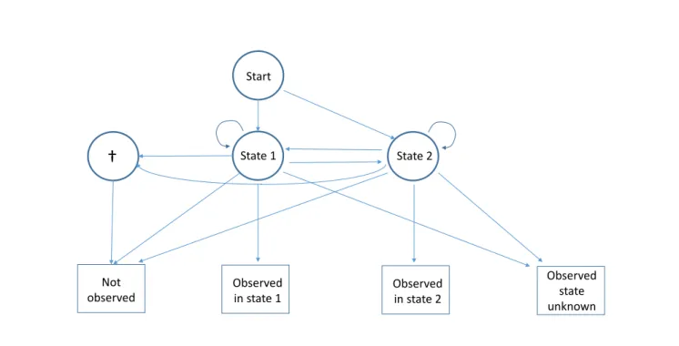
State 1 State 2 Start Not observed Observed in state 1 Observed in state 2 Observed state unknownFigure 1. Diagram of the capture recapture multievent model for partial observations with two observable live states under the null hypothesis. The state ‘dead’ is represented by †. Four events are generated by the three states: ‘Not observed’, which is obligatory for the state ‘dead’; two complete observations, ‘Observed in state 1’ and ‘Observed in state 2’; and the partial observation ‘Observed state unknown’, which may be generated by either live state.
†
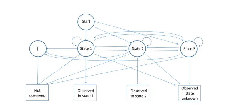
State 1 State 2 Start Not observed Observed in state 1 Observed in state 2 State 3 Observed state unknownFigure 2. Diagram of the capture recapture multievent model for partial observations with two observable live states under the alternative hypothesis where there is one additional non-observable live state (state 3). This last state is never recognized upon observation. See Figure 1 for more details
Table 1. Illustrating how example individual capture histories contribute to the sufficient statistic terms, for a capture-recapture experiment with two observable states A, B and five sampling occasions. Partial observations are denoted by U. The elements of capture history determining the indices within the statistics are denoted in bold.
Capture History sufficient statistic U A U U B wU,−,A1,2 , nA,U U,B2,5
A U U U A nA,U U U,A1,5 A U 0 U 0 v1A U U U U B wU,U U U,B1,5 0 0 U 0 1 w3,5U,0,1 0 A B U U nA,−,B2,3 , v3B 0 U 0 U U bU2
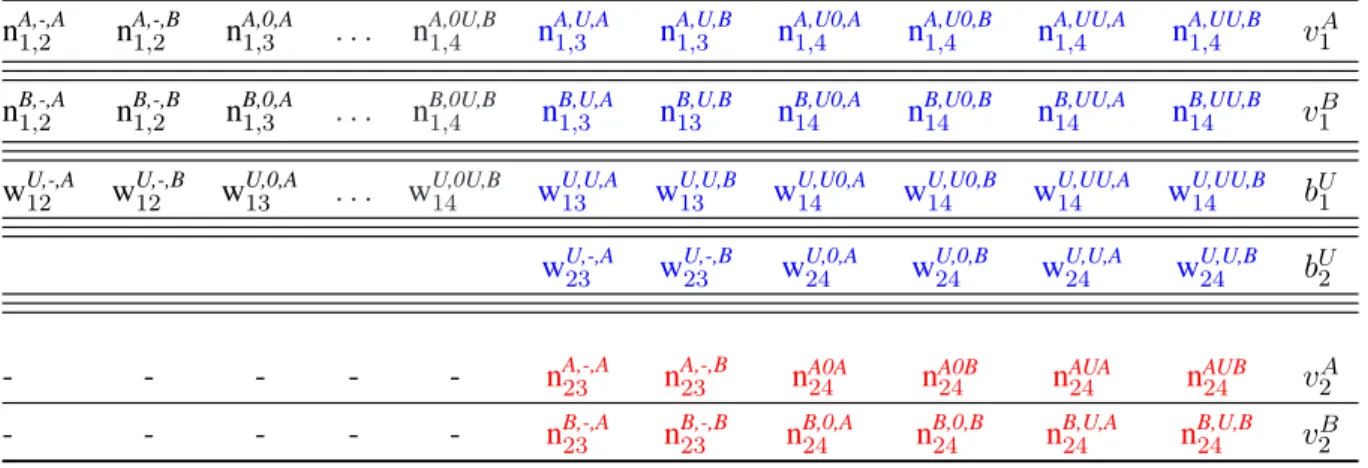
Table 2. The sufficient statistics for multinomial distributions corresponding to individuals released before or at i = 2in an capture-recapture experiment with 4 occasions where individuals can be in any of 2 live states: sufficient-statistic terms.At each time for each individual, one of 4 events occurs: the individual is not encountered (code0), the individual is encountered but its state is not recognized (eventU), the individual is encountered and recognized to be in stateA (codeA), the individual is encountered and recognized to be in stateB(codeB).In the electronic version of the paper the terms constitutive of mixtures are denoted in blue whilst those constituting components are denoted in red. The terms in black will be conditioned upon.bUi -terms are the counts of animals with a first partial observation at i (initial event U ) that are never completely observed. wU,h,Si,j -terms are the counts of animals with a first partial observation at i and a first complete observation at j in state S with intervening capture history h (- stands for the empty capture history). nR,h,Si,j -terms are the counts of animals with two successive complete observations respectively at times i and j in states R and S with intervening capture history h. viS-terms are the counts of animals observed completely for the last time at i in state S.
nA,-,A1,2 nA,-,B1,2 n1,3A,0,A . . . nA,0U,B1,4 nA,U,A1,3 nA,U,B1,3 nA,U0,A1,4 nA,U0,B1,4 nA,UU,A1,4 nA,UU,B1,4 v1A
nB,-,A1,2 nB,-,B1,2 n1,3B,0,A . . . nB,0U,B1,4 nB,U,A1,3 nB,U,B13 nB,U0,A14 nB,U0,B14 nB,UU,A14 nB,UU,B14 v1B
wU,-,A12 wU,-,B12 w13U,0,A . . . wU,0U,B14 wU,U,A13 wU,U,B13 wU,U0,A14 wU,U0,B14 wU,UU,A14 wU,UU,B14 bU1
wU,-,A23 wU,-,B23 wU,0,A24 wU,0,B24 wU,U,A24 wU,U,B24 bU2
- - - nA,-,A23 nA,-,B23 n24A0A nA0B24 nAUA24 nAUB24 v2A - - - nB,-,A23 nB,-,B23 n24B,0,A nB,0,B24 nB,U,A24 nB,U,B24 v2B
Table 3. Table used for testing the mixture property of partial observations at occasion iin a capture-recapture experiment with T occasions where individuals can be in any of R live states. Notations are as in Table 2. The columnscorrespond to the circumstances (time and state) of the first reobservation in a known state after i. They are pooled over the differentinterveningpartial histories(. notation), h(i) = U denotes that the animals are seen in U at i.For individuals seen in U at i,the rows are pooled bylast recognized state at last release (first R rows) and when there are no certaincompleteobservations prior to i+1 (row R+1).For instance, the first row is for animals seen in U at i and with A as their last recognized state; the summation is over the timing of this last previous complete observation.
j = i + 1 . . . T s = A . . . R . . . A . . . R Pi−1 f =1n A,.,A,h(i)=U f,i+1 . . . Pi−1 f =1n A,.,R,h(i)=U f,i+1 . . . Pi−1 f =1n A,.,A,h(i)=U f,T . . . Pi−1 f =1n A,.,R,h(i)=U f,T .. . ... ... ... ... ... ... Pi−1 f =1n R,.,A,h(i)=U f,i+1 . . . Pi−1 f =1n R,.,R,h(i)=U f,i+1 . . . Pi−1 f =1n R,.,A,h(i)=U f,T . . . Pi−1 f =1n R,.,R,h(i)=U f,T Pi f =1w U,.,A,h(i)=U f,i+1 . . . Pi f =1w U,.,R,h(i)=U f,i+1 . . . Pi f =1w U,.,A,h(i)=U f,T . . . Pi f =1w U,.,R,h(i)=U f,T
nA,Ai,i+1 . . . nA,Ri,i+1 . . . nA,.,Ai,T . . . nA,.,Ri,T
..
. ... ... ... ... ... ...
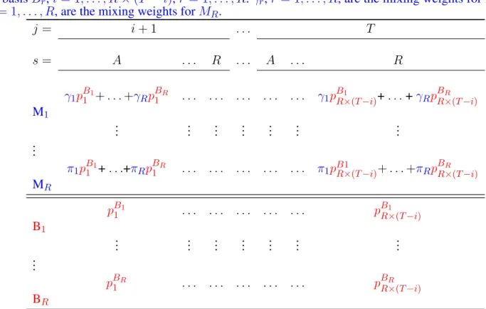
Table 4. Simple model structure of mixtures and associated components used to test the mixture property. In the electronic version of the paper the mixing weights are denoted in blue and the component cell-probabilities in red.Br is the basis corresponding to animals released at i in state r, r = 1, . . . , R. Mr is the mixture corresponding to animals partially observed at i and most lately completely observed in state r, r = 1, . . . , R. Only animals completely reobserved at some point after i are used in the bases and mixtures. The cells of the multinomials correspond to the time and state of the first complete observation after i. They are ordered by states within times for a total of R × (T − i) cells. pBr
i is the probability associated to cell i of basis Br, i = 1, . . . , R × (T − i), r = 1, . . . , R. γr, r = 1, . . . , R, are the mixing weights for M1. πr, r = 1, . . . , R, are the mixing weights for MR.
j = i + 1 . . . T s = A . . . R . . . A . . . R γ1pB11+ . . . +γRpB1R . . . γ1pBR×(T −i)1 + . . . +γRpBR×(T −i)R M1 .. . ... ... ... ... ... ... .. . π1pB11+ . . .+πRpB1R . . . π1pB1R×(T −i)+ . . . +πRpBR×(T −i)R MR pB1 1 . . . p B1 R×(T −i) B1 .. . ... ... ... ... ... ... .. . pBR 1 . . . p BR R×(T −i) BR
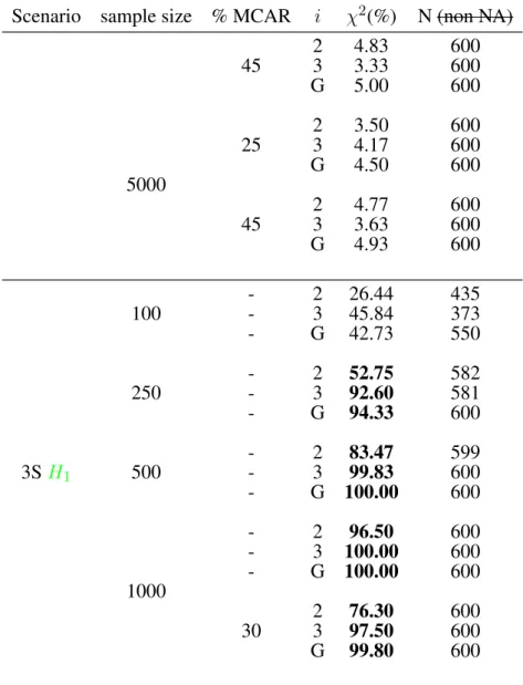
Table 5. Testing the mixture property of partial observations: simulation results. For H0, we generated 2-state capture histories (scenario 2S) examining 2 sample sizes (1000 and 5000 animals newly released per occasion) and 2 percentages of observations rendered partial by setting the state to unknown (%MCAR). Different values of the binomial parameter were considered. ForH1, we generated 3-state capture histories (scenario 3S) examining 4 sample sizes: 2 states were fully observable while the third, never observed, gave rise to all the partial observations. Values of the detection, survival, and transition parameters for scenarios 2S and 3S are given in section 4.1. Under a variant of scenario 3S with the largest sample size, 30% of the observations generated by the 2 observable states are also made partial at random. In all cases, 600 replicates were simulated. Results are given aspercentage of significant test results out of the number of applicable tests(all expected values ≥ 2).G denotes the global test, i the sampling occasion and %M CAR the percentage of observations set to “Unknown” and N denotes the number of applicable tests. The sample size examined is indicated next to the relevant scenario - When 50% or more of the test-results were significant, this is indicated in bold.
Scenario sample size % MCAR i χ2(%) N (non NA)
45 2 4.83 600 3 3.33 600 G 5.00 600 5000 25 2 3.50 600 3 4.17 600 G 4.50 600 45 2 4.77 600 3 3.63 600 G 4.93 600 3SH1 100 - 2 26.44 435 - 3 45.84 373 - G 42.73 550 250 - 2 52.75 582 - 3 92.60 581 - G 94.33 600 500 - 2 83.47 599 - 3 99.83 600 - G 100.00 600 1000 - 2 96.50 600 - 3 100.00 600 - G 100.00 600 30 2 76.30 600 3 97.50 600 G 99.80 600
Table 6. Using different configurations of the Canada geese dataset to assess the performance of the new mixture test for assessing the underlying state structure of partial observations, under real-life conditions. Starting from an original data set where individually identified Canada geese have been observed at 3 locations during 6 consecutive wintering seasons, we artificially generated 3 scenarios underH0 by setting 15%, 25%, and 45% of the observed geese’s locations to unknown : scenarios MCAR15, MCAR25, MCAR45 respectively, and 2 scenarios underH1 by setting all the observations at location 2 (resp. 3) to unknown: scenarios 2PO (resp. 3PO).The p-value obtained at each occasion iis presented and the associated global tests are denoted by G.
Configuration i p-value dfdof
H0 MCAR15 2 0.14 1 3 0.14 1 4 0.60 1 G 0.21 3 MCAR25 2 0.57 1 3 0.09 1 4 0.85 1 G 0.35 3 MCAR45 2 0.84 1 3 0.82 1 4 0.85 1 G 0.99 3 H1 2PO 2 <0.001 1 3 <0.001 1 4 <0.001 1 G <0.001 3 3PO 2 0.13 1 3 <0.001 1 4 <0.001 1 G <0.001 3 Hyb25 2 0.25 1 3 0.28 1 4 0.04 1 G 0.07 3 Hyb45 2 0.37 1 3 0.08 1 4 0.07 1 G 0.06 3