HAL Id: hal-02281865
https://hal.archives-ouvertes.fr/hal-02281865
Submitted on 22 Jan 2020
HAL is a multi-disciplinary open access
archive for the deposit and dissemination of sci-entific research documents, whether they are pub-lished or not. The documents may come from teaching and research institutions in France or abroad, or from public or private research centers.
L’archive ouverte pluridisciplinaire HAL, est destinée au dépôt et à la diffusion de documents scientifiques de niveau recherche, publiés ou non, émanant des établissements d’enseignement et de recherche français ou étrangers, des laboratoires publics ou privés.
The potential of Pléiades images with high angle of
incidence for reconstructing the coastal cliff face in
Normandy
Pauline Letortu, Marion Jaud, Claire Théry, Jean Nabucet, Roza Taouki,
Sophie Passot, Emmanuel Augereau
To cite this version:
Pauline Letortu, Marion Jaud, Claire Théry, Jean Nabucet, Roza Taouki, et al.. The potential of Pléiades images with high angle of incidence for reconstructing the coastal cliff face in Normandy. International Journal of Applied Earth Observation and Geoinformation, Elsevier, 2020, 84, pp.101976. �10.1016/j.jag.2019.101976�. �hal-02281865�
1
The potential of Pléiades images with high angle of incidence for reconstructing
1
the coastal cliff face in Normandy (France)
2 3
Pauline Letortua*, Marion Jauda,b, Claire Thérya, Jean Nabucetc, Roza Taoukia, Sophie Passotd,
4
Emmanuel Augereaua
5 6
aUniversity of Bretagne Occidentale, IUEM, CNRS, UMR 6554 – LETG, Technopôle Brest-Iroise, rue Dumont d’Urville, Plouzané,
7
29280, France, pauline.letortu@univ-brest.fr, claire_thery1@hotmail.fr, Roza.Taouki@ensg.eu,
emmanuel.augereau@univ-8
brest.fr
9
bUniversity of Bretagne Occidentale, IUEM, CNRS, UMS 3113 – IUEM, Technopôle Brest-Iroise, Rue Dumont d'Urville, Plouzané,
10
29280, France, marion.jaud@univ-brest.fr
11
cUniversity of Rennes 2, CNRS, UMR 6554 – LETG, Place du Recteur Henri Le Moal, Rennes, 35000, France,
12
jean.nabucet@uhb.fr
13
dUniversité Claude Bernard Lyon 1, UMR 5276 - Laboratoire de Géologie de Lyon: Terre, Planètes, Environnement, ENS Lyon,
14
Villeurbanne, 69622, France, sophie.passot@univ-lyon1.fr
15
eUniversity of Bretagne Occidentale, IUEM, CNRS, UMR 6538 – IUEM, Technopôle Brest-Iroise, Rue Dumont d'Urville, Plouzané,
16
29280, France
17 18
*Corresponding author. Tel.: +33 290915588, pauline.letortu@univ-brest.fr 19
20
Abstract
21To monitor chalk cliff face along the Normandy coast (NW France) which is prone to erosion, 22
we tested the potential of cliff face 3D reconstruction using pairs of images with high angle of 23
incidence at different dates from the agile Pléiades satellites. The verticality aspect of the cliff 24
face brings difficulties in the 3D reconstruction process. Furthermore, the studied area is 25
challenging mainly because the cliff face is north-oriented (shadow). Pléiades images were 26
acquired over several days (multi-date stereoscopic method) with requested incidence angles 27
until 40°. 3D reconstructions of the cliff face were compared using two software: ASP® and
28
ERDAS IMAGINE®. Our results are twofold. Firstly, despite ASP® provides denser point clouds
29
than ERDAS IMAGINE® (an average of 1.60 points/m² from 40° incidence angle stereoscopic
30
pairs on the whole cliff face of Varengeville-sur-Mer against 0.77 points/m² respectively), 31
ERDAS IMAGINE® provides more reliable point clouds than ASP® (precision assessment on
32
the Varengeville-sur-Mer cliff face of 0.31 m ± 2.53 and 0.39 m ± 4.24 respectively), with a 33
better spatial distribution over the cliff face and a better representation of the cliff face shape. 34
Secondly, the quality of 3D reconstructions depends mostly on the amount of noise from raw 35
images and on the shadow intensity on the cliff face (radiometric quality of images). 36
37
Keywords
38Pléiades imagery; high incidence angle images; cliff face erosion; 3D reconstruction; 39 Normandy 40 41
1. Introduction
42Coastal areas have high density populations due to rich resources and good social and 43
recreational infrastructures. This trend is likely to increase with time but with spatial differences 44
(Neumann et al., 2015). About 52% of the global shoreline is made of cliff coasts that can only 45
retreat (Young and Carilli, 2019). The erosion of these coasts could be dramatic, with 46
occasional massive falls which can threaten people, buildings, utilities and infrastructure 47
located near the coastline (Lim et al., 2005; Naylor et al., 2010; Moses and Robinson, 2011; 48
Kennedy et al., 2014; Letortu et al., 2019). Traditionally, the study of cliff coasts involves 49
quantifying the retreat rates of the cliff top (m/year) with 2D data. This diachronic approach 50
(over several decades) is mainly based on vertical aerial photographs more recently using 51
2
airborne LIDAR data over a significant spatial scale (several tens to hundreds of kilometers) 52
at multi-year intervals (Young, 2018). These average annual retreat rates poorly reflect the 53
erosive dynamics of cliffs, which are characterized by dead time (marine, subaerial, 54
anthropogenic agents weaken the cliff without eroding it) and high points (sudden falls causing 55
cliff retreat). Subsequently, the fall deposit is evacuated by marine action and erosion 56
continues its action on the new cliff face. Scientists have identified the conditions for a better 57
understanding of the regressive dynamics of cliffs (retreat rates, rhythms of evolution, 58
triggering factors of failure). It is necessary to collect 1) 3D data of the cliff face (from the foot 59
to the top of the cliff) to observe all erosion events (2) at high spatial resolution (inframetric) (3) 60
at very high temporal frequency (from seasonal to daily surveys) and (4) over large-scale areas 61
(hydro-sedimentary cell scale for relevant coastal management). 62
While the terrestrial laser scanning and the UAV photogrammetry or terrestrial 63
photogrammetry can meet the first three conditions, the low spatial representativeness of the 64
results is a major constraint (James and Robson, 2012; Letortu et al., 2018; Westoby et al., 65
2018). The boat-based mobile laser scanning data bring together three of the conditions but 66
the cost and the necessary technical know-how limit the temporal frequency of the surveys 67
(Michoud et al., 2014). Moreover, these methods can be very expensive and need staff on the 68
field. Images from Pléiades satellites launched in 2011 and 2012 could be adequate because 69
these satellites are very agile (they can reach a viewing angle of up to 47° to image the cliff 70
face), the data are at very high spatial resolution (around 0.70 m ground sampling distance at 71
nadir for panchromatic images), with a daily revisit frequency and a swath width of 20 km at 72
nadir (ASTRIUM, 2012; Boissin et al., 2012). The images acquired from a pushbroom scanner 73
may be free (under certain conditions) for research institutes and do not require specific 74
fieldwork. 75
In a context of coastal morphology mapping, satellite imagery has long been used for large-76
scale 2D studies, enabling to map shoreline/coastline position and to analyze its evolution (e.g. 77
White and El Asmar, 1999; Boak and Turner, 2005; Gardel and Gratiot, 2006). The 78
development of high-resolution agile satellites has opened up new perspectives, especially for 79
3D reconstruction. Many articles have used Pléiades stereoscopic or tri-stereoscopic 80
acquisitions to answer various scientific questions (e.g. de Franchis et al., 2014; Stumpf et al., 81
2014; Poli et al., 2015) including in coastal environments (AIRBUS, 2015; Collin et al., 2018; 82
Almeida et al., 2019). But, to our knowledge, Pléiades satellite images have never been used 83
in the context of cliff face monitoring which is challenging because it raises four questions: 84
- How to collect Pléiades images on a vertical cliff face? 85
- How to process these high angle of incidence images? 86
- What is the relevance of this data for cliff face 3D reconstruction (sufficient point density on 87
the cliff face to observe structural discontinuities)? 88
- What are the favorable acquisition parameters and site characteristics for cliff face surveys 89
(angle of incidence, season, orientation of the coastline, color of the cliff face)? 90
For this study, images were acquired along the Norman coastal cliffs (Seine-Maritime), from 91
Quiberville to Berneval-le-Grand (20 km, north-oriented cliff face) because the risk of erosion 92
is significant. The fast retreat rate of chalk cliffs has reached urban areas and impacted the 93
local use of the beach. Some areas are under expropriation procedures to protect populations 94
(Dieppe) and a fatality occurred in August 2015 in Varengeville-sur-Mer where a shell 95
fisherman died after being buried by tons of rock due to chalk cliff fall. One of the challenges 96
in coastal management is to predict the coastal evolution in order to protect people living in 97
this environment. This challenge can be achieved using relevant, homogeneous and long-term 98
data including these provided by Pléiades imagery. 99
3
The standard stereoscopic or tri-stereoscopic acquisition which consists, within the same pass 100
of the satellite on its meridian orbit, of acquiring two or three images over the area of interest 101
(front, nadir and back images) is proved unsuitable in our case because of the orientation of 102
the cliff face: the backward viewing image would capture the plateau but not the cliff face 103
making 3D reconstruction impossible. Furthermore, the studied cliff face being a sub-vertical 104
object, a high angle of incidence should be favorable. Thus, we imagined an original acquisition 105
procedure: as the orbital pass position changes daily, a multi-date survey over several 106
consecutive days, with mono-acquisition and a high angle of incidence (across-track), was 107
performed to observe the area at various viewing angles. In order to assess the impact of the 108
angle of incidence, two sets of images were simultaneously requested: one with a pitch 109
imaging angle of 40° and the second one with a pitch imaging angle between 0° and 10°. 110
First, the study area will be described, followed by the methods of acquisition and data 111
processing of images with a high angle of incidence. In a third step, the results of our 112
exploratory research on the relevance of Pléiades data for reconstructing the Norman cliff face 113
and the favorable acquisition parameters and site characteristics will be presented and 114
discussed. Conclusions will be drawn in the final section. 115
116
2. Study area
117The study area is located in north-western France (01°00’E; 49°55’N), in Normandy (Seine-118
Maritime), along the Channel. Climatically, the area belongs to the western part of Europe 119
which is particularly exposed to the influences of oceanic low pressures, and thus, to the types 120
of disturbed weather that dominate approximately 2/3 of the year (Pédelaborde, 1958; Trzpit, 121
1970). Geologically, it belongs to the northeastern part of the Parisian Basin (sedimentary), 122
where the Pays de Caux plateau abruptly ends in subvertical coastal cliffs. Cliffs are made of 123
Upper Cretaceous chalk with flints (Pomerol et al., 1987; Mortimore et al., 2004). The altitude 124
range of the cliffs is between 20 m to 100 m with an increase from south-west to north-east, 125
and locally cut by valleys. As shown in Figure 1, these cliffs are mainly white in color, but the 126
sub-vertical cliffs are darkened (brown color) by a bed of clay and sand sediment of the Tertiary 127
Period (Paleogene) between Sainte-Marguerite-sur-Mer and Dieppe, and elsewhere by clay-128
flint formations above the chalk strata. The average tidal range is 8 m (macrotidal environment). 129
At low tide the foreshore is characterized by a wide shore platform slightly inclined to the sea 130
with a gravel barrier near the cliff foot contact. 131
4 133
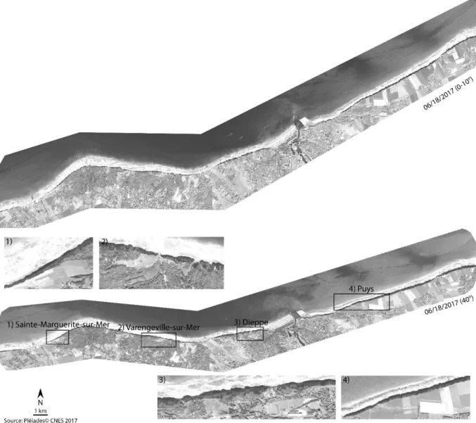
Figure 1 : Presentation of the study area from Quiberville to Berneval-le-Grand (Seine-Maritime, 134
Normandy) 135
136
Along the studied coastline (between Quiberville and Berneval-le-Grand, 20-km long), the 137
lithology of the cliffs from Sainte-Marguerite-sur-Mer to Dieppe is composed of Santonian and 138
Campanian chalk and covered by Paleogene strata. The lithology is prone to erosion with the 139
highest annual retreat rate (0.23 m/year) in comparison with average county retreat rate (0.15 140
m/year between Cap d’Antifer and Le Tréport, 1966-2008 (Letortu et al., 2014)). Between 141
Dieppe and Berneval-le-Grand (Turonian and Coniacian chalk stages), the retreat rate is lower 142
(0.12 m/year). The modalities of erosion are varied with falls of a few m3 to hundreds of
143
thousands of m3 but they are ubiquitous along the cliff line.
144
The study area is challenging for the acquisition of these satellite images because (1) the 145
SW/NE orientation of the coastline complicates the image acquisition while the Pléiades orbit 146
is meridian; (2) the cliff face is north-oriented, so in the cast shadow during the satellite passing 147
time, even in summer; (3) the weather conditions are often cloudy and rainy in the area 148
because it is located in mid-latitudes where disturbed weather dominates; (4) a high tidal range 149
limits the acquisition periods because the whole cliff face is needed. 150
For the 3D reconstruction, the diversity of cliff types along the 20 km cliff line is also challenging. 151
To assess the quality of reconstructions in function of the site characteristics, four areas of 152
interest (AOIs) were selected: Sainte-Marguerite-sur-Mer, Varengeville-sur-Mer, Dieppe and 153
Puys (Table 1, Figure 2). The whitest cliff faces are located at Puys. The cliff face colors at 154
Sainte-Marguerite-sur-Mer, Varengeville-sur-Mer and Dieppe are from brown to light gray. The 155
shore platform is gray or beige and mainly rocky with gravel accumulation except at Puys, 156
where there are no gravel accumulations. Sainte-Marguerite-sur-Mer and Varengeville-sur-157
Mer have the lowest cliff height (from 20 to 40 m), with the gentlest cliff face slope at Sainte-158
Marguerite-sur-Mer (70°). Sainte-Marguerite-sur-Mer and Puys have a sublinear coastline 159
5
(average depth of incisions from 10 to 20 m) whereas Varengeville-sur-Mer and Dieppe have 160
a jagged coastline (incisions from 75 to 115 m-deep) (Figure 2). 161 162 Area of interest (AOI) Sainte-Marguerite-sur-Mer (00°56’37”E; 49°54’42”N) Varengeville-sur-Mer (01°00’22”E; 49°55’01”N) Dieppe (01°03’33”E; 49°55’27”N) Puys (01°07’26”E; 49°56’38”N) Cliff face color Ochre and light gray Brown and light gray Brown and light gray Light gray Shore platform
color Dark gray Beige Dark gray Light gray
Type of platform
Rocky and gravel accumulation
Rocky and gravel accumulation
Rocky and gravel
accumulation Rocky Average cliff height (m) 20-50 30-40 60 70 Average cliff face slope (°) 70 70-90 80-85 80-90 Orientation of
cliff face NW NNE NNW NNW
Average depth of incision*
(m)
10 115 75 20
Table 1: Main characteristics of the AOI sites (*the depth of incision is the length from the headland to 163
the trough (perpendicular to the coastline)) 164
165
Figure 2: Images acquired on 06/18/2017 with both requested incidence angles and the location of 166
AOIs 167
6 168
3. Data collection and processing
1693.1. Acquisition strategy 170
The high angle of incidence needed for the images of the multi-date survey requires the 171
satellite position at the time of acquisition to be above the Channel or the United Kingdom 172
(Figure 3). This means that cloud cover must be from zero to low over large areas, around 173
11:25 UTC (satellite pass time). 174
175
176
Figure 3: Principle of the multi-date survey used in this study 177
In this configuration, the acquisition is considered challenging by the image supplier due to the 178
high incidence angle, repetitiveness and short periods of time when the site is accessible under 179
good conditions (zero or low cloud cover (between 0 and 10%) and during low tide if possible). 180
181
3.2. Acquired images and stereo-pairs 182
In order to follow the evolution of the studied cliffs, different periods were chosen for Pléiades 183
image acquisition: 184
- Fall 2016: 4 stereoscopic pairs; 185
- Summer 2017: 5 stereoscopic pairs (Figure 2); 186
- Winter 2017/2018: 5 stereoscopic pairs. 187
The angle of incidence is different from the viewing angle due to the sphericity of the Earth. To 188
limit the differences induced by the geometric configuration of the images, we chose to perform 189
3D reconstruction from images acquired with similar incidence angles (either 40° or 0-10°). 190
The images acquired (Table 2) used in this paper are panchromatic ones, as spatial resolution 191
is finer (0.7 m) than multispectral images (2.8 m). However, due to the geometry of acquisition, 192
the ground sampling distance is variable from one day to another, varying for example from 193
0.27 m to 1.83 m for images at 40° of incidence. 194
7 Date Hour (UTC) Name of satellite Requested incidence angle Weather Pitch viewing angle (°) Roll viewing angle (°) Pitch incidence angle (°) Roll incidence angle (°) Oblique distance between the satellite and the
cliff (m) 10/05/2016 11:29 1B 0-10 Sunny 2.25 29.16 12,96 -3.01 707856 10/06/2016 11:21 1A 0-10 Cloudy 4.78 20.75 -11.50 -21.13 727351 10/08/2016 11:06 1A 0-10 Sunny -0.7 0.9 0.74 -1.16 694160 10/31/2016 11:29 1B 0-10 Sunny -1.06 29.28 -9.49 -31.98 700857 06/10/2017 11:21 1B 0-10 Sunny 9.65 20.6 -16.56 -19.65 743652 06/15/2017 11:33 1B 0-10 Sunny 1.01 32.83 -11.75 -35.9 703506 06/18/2017 11:10 1A 0-10 Sunny 3.07 6.47 -4.6 -5.39 698687 07/06/2017 11:21 1B 0-10 Cloudy 9.13 20.45 -15.95 -19.64 742090 07/21/2017 11:06 1A 0-10 Sunny 9.71 0.17 -10.4 2.2 916552 12/01/2017 11:32 1A 0-10 Cloudy 30.47 31.29 -11.75 -35.86 884638 12/16/2017 11:17 1B 0-10 Cloudy 9.71 15.72 -14.78 -14.35 759203 01/24/2018 11:17 1A 0-10 Cloudy -0.66 16.09 -3.88 -17.54 731573 02/12/2018 11:20 1A 0-10 Cloudy 9.15 20.34 -15.93 -19.51 742410 02/17/2018 11:32 1A 0-10 Sunny 5.91 32.44 -18.71 -33.79 720932 10/05/2016 11:27 1B 40 Sunny 40.65 26.65 -50.56 -15.94 1023748 10/06/2016 11:20 1A 40 Cloudy 30.39 19.35 -37.59 -11.93 884387 10/08/2016 11:05 1A 40 Cloudy 34,15 0.7 -37.55 10.79 850050 10/31/2016 11:28 1B 40 Misty 30.39 27.7 -40.49 -21.52 878726 06/10/2017 11:20 1B 40 Sunny 40.69 18.35 -48.5 -6.23 1026143 06/15/2017 11:31 1B 40 Sunny 30.48 31.32 -42.09 -25.81 884838 06/18/2017 11:08 1A 40 Sunny 37.32 3.83 -41.92 7.65 890433 07/06/2017 11:20 1B 40 Sunny 30.46 19.22 -37.62 -11.77 885380 07/21/2017 11:05 1A 40 Sunny with scattered clouds 39.24 1.42 -43.56 13.63 704437 12/01/2017 11:31 1A 40 Cloudy -1.03 32.79 -42.08 -25.74 703402 12/16/2017 11:17 1B 40 Cloudy 30.43 14.5 -36.34 -6.6 896286 01/24/2018 11:16 1A 40 Cloudy 30.48 14.46 -36.38 -6.57 896897 02/12/2018 11:20 1A 40 Cloudy 30.46 19.11 -37.59 -11.67 885643 02/17/2018 11:30 1A 40 Sunny 36.03 30.63 -47.2 -22.92 954538
Table 2: Characteristics of acquired Pléiades images 196
197
For the 3D reconstruction of the cliff face, the 0-10° and 40° images were examined according 198
to three criteria to select the stereoscopic pairs which appeared relevant to process: 199
- The absence of rock falls between both images: Thus, a study of falls on the AOIs between 200
2016 and 2018 identified one fall at Varengeville-sur-Mer on 10/23/2017, two falls at Sainte-201
Marguerite-sur-Mer (one between 07/21/2017 and 12/12/2017, the other between 07/21/2017 202
and 12/01/2018), one fall at Puys (between 01/24/2018 and 02/12/2018). It is possible that 203
some falls were missed, therefore it was decided that the acquisition period for stereoscopic 204
image pairs should not exceed 2 months; 205
- Good image quality: A clear sky is required between the satellite and the study area to have 206
a cloud-free imagery (Berthier et al., 2014), thus a satisfactory radiometric quality. This 207
statement is also true for the cliff shadow. In our study area, a good radiometric quality (values 208
of the pixels vary from 0 to 4095 for 12 bit images) is between 134 and 827 for the mean value 209
and between 177 and 1543 for the standard deviation. Meteorology and the size of the shadow 210
on the cliff face have been grouped together under the parameter "visual image evaluation". 211
Only images with good visual image evaluation were retained. 212
- The “flattening” coefficient of the pixels must be limited: where pixel flattening 213
coefficient=Image resolution (x)/Image resolution (y). In our study, flattening coefficient has to 214
be between 0.22 and 2.23 to facilitate feature recognition between images. Not surprisingly, 215
8
the flattening of the pixels is much less marked at 10° than at 40° (on average 0.92 at 0-216
10°and 0.55 at 40°). 217
Taking into account these three criteria, 23 image pairs were tested (Table 3). 218
219
Date of stereoscopic pairs Incidence angles (°)
06/10/2017 06/15/2017 0-10 06/15/2017 07/06/2017 0-10 12/01/2017 12/16/2017 0-10 01/24/2018 02/12/2018 0-10 01/24/2018 02/17/2018 0-10 02/12/2018 02/17/2018 0-10 10/05/2016 10/08/2016 40 10/05/2016 10/31/2016 40 10/08/2016 10/31/2016 40 06/10/2017 06/15/2017 40 06/10/2017 06/18/2017 40 06/10/2017 07/06/2017 40 06/15/2017 06/18/2017 40 06/15/2017 07/06/2017 40 06/15/2017 07/21/2017 40 06/18/2017 07/06/2017 40 06/18/2017 07/21/2017 40 07/06/2017 07/21/2017 40 12/01/2017 12/16/2017 40 12/01/2017 01/24/2018 40 01/24/2018 02/12/2018 40 01/24/2018 02/17/2018 40 02/12/2018 02/17/2018 40
Table 3: Stereoscopic pairs used for data processing 220
3.3. Data processing 221
Usually, different software (commercial and open-source) can be used for 3D reconstruction 222
but, in our case, the unusual configuration of images may restrict the choice of suitable 223
software. 224
In this study, an open-source (ASP® 3.5.1) and a commercial software (ERDAS IMAGINE ®)
225
were used. ERDAS IMAGINE® is a commercial software suite for the creation, visualization,
226
geocorrection, reprojection and compression of geospatial data. ASP® (Ames Stereo Pipelines,
227
NASA) is a suite of free and open-source automated geodesy and stereogrammetry tools 228
(Shean et al., 2016) notably developed for satellite imagery with very detailed documentation 229
(NASA, 2019,
https://ti.arc.nasa.gov/tech/asr/groups/intelligent-230
robotics/ngt/stereo/#Documentation). 231
Internal and external parameters of the pushbroom sensor are provided with each image. They 232
are empirically described using rational polynomial camera model. Images are provided with 233
Rational Polynomial Coefficients (RPCs), approximating functions which describe the 234
relationship between image space and object space (de Franchis et al., 2014). RPCs are 235
accurate only within a specified validity zone and can reveal inconsistencies for large scenes 236
and/or multi-temporal acquisitions (Rupnik et al., 2016). Both ERDAS IMAGINE® and ASP®
237
use RPC sensor model to perform orthorectification and georectification. For some processing 238
chains, RPCs are computed or affined using Ground Control Points (GCPs) collected 239
9
throughout the area (Salvini et al., 2004; Kotov et al., 2017). In our case, no GCPs were used 240
and the RPC-based sensor orientation was only refined using tie points identified on both 241
images of the pair. 242
In ERDAS IMAGINE®, automatic tie point detection provided poor results probably due to high
243
incidence angles and multi-date images. To improve detection, we manually pointed tie points 244
on each image. A minimum of 25 points was chosen (optimal threshold defined after trials 245
between availability of relevant tie points and quality of Root Mean Square Error (RMSE)). 246
These points are preferably identifiable and unchangeable elements on flat areas, where 247
distortions are limited (middle of a crossroads rather than a house roof). In addition, tie points 248
are mainly located near the coast in order to minimize correlation errors over this area of 249
interest. A polynomial model is considered satisfactory when all the points have a RMSE 250
inferior to 0.5 pixels (Vanderstraete et al., 2003). When the RMSE of the triangulation ratio was 251
greater than 0.5 pixels or when the uncertainty threshold was greater than 4 meters for a tie 252
point, it was systematically removed and replaced by a better point. In ASP®, we skipped this
253
step because co-registration using a rigid-body transformation can accomplish similar results 254
with reduced processing time (Shean et al., 2016). 255
Epipolar images are then computed to perform stereo-matching in both software (Normalized 256
Cross Correlation algorithm in ERDAS IMAGINE®, More Global Matching (MGM) one in ASP®).
257
This stereo-matching step consists of cross-correlation to identify pixel correspondences 258
between the left and right epipolar images. Given characteristic variations of the stereoscopic 259
pairs (multi-date), it is difficult to standardize the processing parameters within the software 260
and between software. As the areas of interest correspond to steep slopes, we used small 261
correlation windows (7*7 pixels, 9*9 pixels). The small size of the windows may introduce more 262
false matches or noise (NASA, 2019). Because of the shadow on the cliff face, the “low contrast” 263
parameter was activated in ERDAS IMAGINE® during the image matching to force it to find tie
264
points in this area. In ASP®, the MGM algorithm was used to decrease high frequency artifacts
265
in low texture areas in order to find more corresponding pixels between both images. 266
Sub-pixel refinement was used in ERDAS IMAGINE® (Least Square Refinement) whereas it
267
was not used in ASP® in order to reduce processing time (Shean et al., 2016) without altering
268
quality of our results. 269
In ASP®, we used post filtering to filter disparity (artifacts) with three filters: median-filter-size
270
(3 pixels), texture-smooth-size (11 pixels) and texture-smooth-scale (0.15 pixels). 271
Finally, a 3D position can be computed for each pair of corresponding pixels. The software 272
also generate a DEM, but considering the verticality of the cliff face, we only exported the 3D 273
point cloud. 274
The point clouds are then post-processed with CloudCompare®, an open-source software, to
275
manually filter artifacts in the point cloud. 276
To assess the impact of the study site characteristics and of the acquisition parameters, the 277
parameterization of both software was not changed from one stereoscopic pair to another or 278
from one AOI to another. 279
280
4. Results and discussion 281
4.1. Comparison of the results provided by the different processing 282
4.1.1. Point density 283
In order to have a relevant cliff face monitoring, it is necessary that the whole cliff face is 284
sampled during 3D reconstruction with sufficient resolution to observe the structural 285
discontinuities of the cliff face. The average density of the point clouds corresponding to the 286
Varengeville-sur-Mer cliff face is calculated (Table 4). The point density is much higher for 3D 287
10
reconstructions made with ASP® than ERDAS IMAGINE® (respectively, 1.86 points/m² versus
288
0.24 points/m² on the whole cliff face for 0-10° of incidence angle and 1.60 points/m² versus 289
0.77 points/m² for 40° of incidence angle). Regardless of the angle of the images and the used 290
software, the cliff foot is the least densely reconstructed part (0.74 points/m² with ASP® and
291
0.04 points/m² with ERDAS IMAGINE® for a pair of images at 0-10°) while the most
292
reconstructed part is the cliff top (1.37 points/m² with ASP® and 0.89 points/m² with ERDAS
293
IMAGINE® for a pair of images at 40°). This point density difference might be due to the
294
correlation step using different algorithms. 295
296
Location on the cliff face Requested incidence angles used for 3D reconstruction
Average point density (number of points/m²) with
ASP®
Average point density (number of points/m²) with
ERDAS IMAGINE®
Cliff top 0-10° 1.87 0.15
40° 1.37 0.89
Middle of the cliff face 0-10° 1.64 0.13
40° 1.45 0.67
Cliff foot 0-10° 0.74 0.04
40° 1.03 0.25
Whole cliff face 0-10° 1.86 0.24
40° 1.60 0.77
Table 4: Average density of the point clouds in Varengeville-sur-Mer in function of the cliff face part 297
and the used software 298
299
4.1.2. Point distribution 300
The point distribution of the 3D reconstructions obtained on the cliff face with both software is 301
different (Figure 4). Although the point cloud obtained with ASP® is denser than that obtained
302
with ERDAS IMAGINE®, the shape of the cliff is more realistic with ERDAS IMAGINE® (see
303
dotted black frames in Figure 4). 304
With ASP®, there are very few artifacts on the plateau and on the platform. They are mainly
305
located on edges of the point cloud and at shadow/sunlit contact (white dotted circles depict 306
areas where the contact is located about 20 m from the foot of the cliff (Figure 4)). At this latter 307
area, artifacts have the shape of a stair step. 308
For ERDAS, there are spike-shaped artifacts on the plateau but also on the platform because 309
the optimization of processing parameters is focused on the cliff face and is not suitable for the 310
whole area. These artifacts make cleaning difficult. In the shadow/sunlit contact, the points are 311
higher than the rest of the points on the platform. 312
The 3D reconstruction obtained with ASP® was filtered (data deleted in post-processing with
313
CloudCompare®) in the circles because of an unrealistic stair-step artifact. The 3D
314
reconstruction from ERDAS IMAGINE® is not very dense within the circles, but the few
315
scattered points allow realistic observation of the cliff foot (Figure 4). 316
11 318
Figure 4: Distribution of points of the reconstructed cliff faces from the stereoscopic pair on 06/18/2017 319
and 07/06/2017 with a requested incidence angle of 40° at Varengeville-sur-Mer. The white dotted 320
circles depict areas where the shadow/sunlit contact is located about 20 m from the foot of the cliff, thus 321
where reconstruction is challenging. 322
323
4.1.3. Planimetric precision assessment 324
To georeference the point clouds from Pléiades images and compare them to multi-source 325
data (UAV, TLS…), we proceeded to a semi-automatic co-registration using a rigid-body 326
transform. This co-registration is efficiently constrained vertically (shore platform, plateau) and 327
alongshore. Thus, precision error is assessed in the cross-shore direction (which is the 328
direction of erosion on the cliff face). 329
The precision assessment is performed on the AOI of Varengeville-sur-Mer because UAV data 330
were acquired on 06/26/2017 (by Azur Drones Company for RICOCHET research project). 331
The precision assessment is based on the relative distance (normal of the cliff face) after fitting 332
(Iterative Closest Point algorithm in Cloudcompare®) between the 3D point cloud reconstructed
333
from Pléiades images (11 stereoscopic pairs in June and July 2017) and the one from UAV 334
images (model). These synchronous surveys allow to limit errors due to erosion events. Table 335
5 summarizes the relative precision of the cliff face reconstructions. 336
337
Date of stereoscopic pairs Requested incidence angle used for 3D reconstruction Average relative distance (normal of cliff face) [standard deviation] with ASP® Average relative distance (normal of cliff
face) [standard deviation] with ERDAS IMAGINE®
06/10/2017 06/15/2017 0-10° 0.10 [4.94] 0.45. [2.69]
06/15/2017 07/06/2017 0-10° 0.05 [4.45] 0.06 [2.34]
06/10/2017 06/15/2017 40° 0.76 [3.88] 0.43 [3.04]
12 06/10/2017 07/06/2017 40° -0.23 [3.59] 0.00 [2.81] 06/15/2017 07/21/2017 40° 0.89 [4.99] 0.62 [2.85] 06/15/2017 06/18/2017 40° -0.01 [4.02] 0.57 [2.44] 06/15/2017 07/06/2017 40° 0.17 [4.62] -0.09 [2.11] 06/18/2017 07/06/2017 40° 1.03 [4.04] 0.25 [1.86] 06/18/2017 07/21/2017 40° 1.23 [4.65] -0.37 [2.82] 07/06/2017 07/21/2017 40° 0.07 [3.89] 0.63 [2.39]
Average relative distance (normal of cliff face) for the 11 stereoscopic pairs
[average standard deviation]
0.39 [4.24] 0.31 [2.53]
Table 5: Relative distance of cliff face normal at Varengeville-sur-Mer between 3D reconstruction from 338
Pléiades images (stereoscopic pairs in June and July 2017) and the one from UAV images 339
(06/26/2017) 340
The precision of the cliff face reconstruction is slightly better with ERDAS IMAGINE® than ASP®
341
(average relative distance of 0.31 m and 0.39 m respectively). Furthermore, the standard 342
deviations are lower with ERDAS IMAGINE® than with ASP® (average standard deviation of
343
2.53 and 4.24 m respectively). With a better average precision associated with a low error 344
dispersion on the cliff face, the 3D reconstruction with ERDAS IMAGINE® provides a reliable
345
dataset. Nevertheless, these better results in precision can partly originate from lower point 346
density of the ERDAS® point clouds than of ASP® point clouds.
347
Regardless of the processing software used, the precision of the cliff face reconstruction is 348
better for acquisitions with a 0-10° incidence angle than with a 40° angle. Indeed, low angles 349
of incidence can limit distortions and inaccuracies of the RPC-based sensor orientation. 350
The spatial distribution of the relative distance between cliff face reconstruction and UAV data 351
is different in function of the software (Figure 5). The 3D reconstruction obtained with ASP®
352
creates a difference of more than 10 m at the foot of the cliff, where an artifact in the shape of 353
a stair step appears because of the shadow. Concerning the 3D reconstruction obtained with 354
ERDAS IMAGINE®, the large differences (greater than 6 m) are scarce and mainly randomly
355
distributed over the whole cliff face. These artifacts can be removed by manual filtering. 356
13 358
Figure 5: Relative distance of the cliff face normal (in m) at Varengeville-sur-Mer between 3D 359
reconstructions with ERDAS IMAGINE® and ASP® (stereoscopic pair on 06/18/2017 and 07/06/2017
360
acquired at 40° requested incidence angle) in comparison with UAV data (06/26/2017) 361
362
In our study, despite a higher point density of the ASP® reconstruction compared to ERDAS
363
IMAGINE® one, the latter software is more suitable because the reconstructed points are more
364
precise and better distributed over the cliff face, providing a reliable dataset. 365
366
4.2. Identification of image pairs which give satisfactory reconstruction of the cliff face 367
First of all, the quality of 3D reconstruction of the cliff face proved to be less relevant than 368
expected. Based on the point resolution on the cliff face, many couples have "unusable" 369
reconstructions with very few points on the cliff face (< 1 pt/30 m) and/or with a proportion of 370
computational artifacts greater than or equal to the proportion of valid points. Computational 371
artifacts can be due to unsuitable geometry of acquisition between the images of the couple or 372
bad tie point detection during correlation. Thus, for "usable" 3D reconstructions, less restrictive 373
thresholds have been put in place: 374
- "few satisfactory" when the density is < 1 pt/15 m but a good signal to noise ratio; 375
- "satisfactory" when the density is > 1 pt/15 m (Figure 6). 376
14 378
Figure 6: Ranking of 3D reconstruction quality of the cliff face in Varengeville-sur-Mer 379
380
The last threshold allows visibility of structural discontinuities from the cliff foot to the cliff top. 381
Since ERDAS IMAGINE® creates reliable 3D reconstruction, this software is used to sort the
382
different image pairs on the different AOI (Table 6). 383 384 Image 1 Image 2 Set of images (°) Sainte- Marguerite-sur-Mer
Varengeville-sur-Mer Dieppe Puys
06/10/2017 06/15/2017 0-10 few satisfactory few satisfactory satisfactory satisfactory 06/15/2017 07/06/2017 0-10 few satisfactory satisfactory satisfactory satisfactory 12/01/2017 12/16/2017 0-10 unusable unusable unusable unusable 01/24/2018 02/12/2018 0-10 unusable unusable unusable few satisfactory 01/24/2018 02/17/2018 0-10 unusable unusable unusable unusable 02/12/2018 02/17/2018 0-10 unusable unusable unusable unusable
10/05/2016 10/08/2016 40 unusable unusable unusable unusable
10/05/2016 10/31/2016 40 unusable unusable unusable unusable
10/08/2016 10/31/2016 40 few satisfactory unusable unusable unusable 06/10/2017 06/15/2017 40 few satisfactory satisfactory satisfactory few satisfactory 06/10/2017 06/18/2017 40 satisfactory satisfactory satisfactory satisfactory 06/10/2017 07/06/2017 40 few satisfactory satisfactory satisfactory satisfactory 06/15/2017 06/18/2017 40 few satisfactory satisfactory satisfactory few satisfactory 06/15/2017 07/21/2017 40 few satisfactory satisfactory unusable unusable 06/15/2017 07/06/2017 40 satisfactory satisfactory satisfactory satisfactory 06/18/2017 07/06/2017 40 few satisfactory satisfactory satisfactory satisfactory 06/18/2017 07/21/2017 40 satisfactory satisfactory unusable unusable 07/06/2017 07/21/2017 40 unusable satisfactory satisfactory unusable
15
12/01/2017 01/24/2018 40 unusable unusable few satisfactory unusable
01/24/2018 02/12/2018 40 unusable unusable unusable unusable
01/24/2018 02/17/2018 40 unusable unusable satisfactory unusable
02/12/2018 02/17/2018 40 unusable unusable unusable unusable
Table 6: Quality of cliff face 3D reconstructions on ERDAS IMAGINE® in function of the 23
385
stereoscopic pairs 386
On the 92 tests, 29 give satisfactory 3D reconstruction (as in Figures 4 and 5), 13 are few 387
satisfactory and the rest is unusable. Stereoscopic pairs at 40° provide more satisfactory 3D 388
reconstruction over the four AOIs than stereoscopic pairs at 0-10°. Of the six stereoscopic 389
pairs at 0-10°, two pairs give satisfactory results on two or three AOIs (mainly Dieppe and 390
Puys). On 23 stereoscopic pairs at 40°, 10 pairs give satisfactory results, mainly on two areas 391
of interest (Varengeville-sur-Mer and Dieppe). Two image pairs have satisfactory 3D 392
reconstruction on the four AOIs: 06/10/2017-06/18/2017 and 06/15/2017-07/06/2017. 393
394
4.3. Identification of radiometric and geometric acquisition parameters favorable for 3D 395
reconstruction of the cliff face 396
Unsurprisingly, the best images for cliff face reconstruction are those with: 397
- Sunny weather (e.g. 06/18/2017 and 07/06/2017 in Figures 4 and 5); 398
- Few shadows on the cliff face. 399
Both parameters are relevant for a satisfactory tie point detection because they provide various 400
radiometric information. Over the four AOIs, the average radiometry of images which give 401
satisfactory 3D reconstruction is between 300 and 400, whereas the standard deviation is 402
between 80 and 94. This corresponds to a favorable ratio « mean/standard deviation » inferior 403
to 5. 404
The main problem encountered in the 3D reconstruction is the cast shadow phenomenon on 405
the cliff face (umbra and penumbra) that causes the partial or total loss of radiometric 406
information (Arévalo et al., 2006). The summer season is the best period to limit this 407
phenomenon, although it cannot be totally avoided because of the north-facing cliff along the 408
studied coastline. Our current results mean that summer acquisitions are the most appropriate 409
whereas a high temporal frequency is needed by scientists (from daily to seasonal surveys). 410
In recent years several techniques have been studied to detect shadow areas and to 411
compensate the loss of radiometric information or reconstruct it (for a review Shahtahmassebi 412
et al., 2013; Al-Helaly and Muhsin, 2017). Shadow detection methods (thresholding, modeling, 413
invariant color model, shade relief), and de-shadowing methods (e.g. visual analysis, 414
mathematical models, fusion and data mining techniques) will be tested to improve radiometric 415
information for better tie point detection and so higher quality 3D reconstruction. 416
For the geometric acquisition parameters, satisfactory reconstruction also comes from 417
stereoscopic pairs at 0-10° but, with ERDAS IMAGINE®, the cliff face sampling distance is less
418
satisfactory than for reconstruction from 40° stereoscopic pairs. However, the shortest distance 419
between satellite/cliff face at 0-10° incidence angle than at 40° is prone to limited cloud cover. 420
It may therefore be interesting to find a compromise between the incidence angle of images 421
(from 10° to 40°) and the cliff face ground sampling. 3D cliff face reconstructions made by UAV 422
images on the same study area show that 20°, 30° and 40° off-nadir imaging angles provide 423
satisfactory results in terms of accuracy and texture restitution (Jaud et al., 2019). Therefore, 424
a compromise with an angle of incidence of 20° seems promising and will be tested. 425
Furthermore, because of the radiometric variations (different illumination conditions) and 426
16
geometric ones (in across-track direction) in multi-date stereoscopic pairs with the same 427
incidence angle, it would be interesting to test 3D reconstruction from pairs of images acquired 428
the same day at 0-10° and 40° (same radiometric configuration, but geometric variations in 429
along-track direction). 430
431
4.4. Identification of site parameters most suitable for 3D reconstruction of the cliff face 432
The best reconstructed cliff faces are those in Dieppe and Varengeville-sur-Mer with 10 433
satisfactory 3D reconstructions (Table 6). This can be explained by the highest depths of 434
incision (75 m at Dieppe and 115 m at Varengeville-sur-Mer) and the variability of the cliff face 435
color (high standard deviations in radiometry, 103 and 124 at Varengeville-sur-Mer and Dieppe 436
respectively) which allow easy detection of tie points due to texture change (Figure 4). 437
438
5. Conclusions
439In this exploratory research, the potential of Pléiades satellite images to monitor coastal cliff 440
face was investigated. The study area in Normandy (from Quiberville to Berneval-le-Grand) is 441
particularly challenging because of its orientation (north-oriented cliff face) and the high 442
frequency of cloud cover. To obtain images with high angle of incidence of the cliff face, a 443
multi-date acquisition was specifically designed. The images with a high angle of incidence 444
(from nadir to 40°) were processed using ASP® and ERDAS IMAGINE®. Interesting 3D
445
reconstructions are obtained, especially with ERDAS IMAGINE® which provides more precise
446
reconstructed points than ASP® (average relative distance and standard deviation of 0.31 m ±
447
2.53 and 0.39 m ± 4.24 respectively) and better distributed over the cliff face providing a 448
reliable dataset. In our study, a minimum of 1 pt/15 m allows visibility of structural 449
discontinuities from the cliff foot to the cliff top. Most of the satisfactory 3D point clouds come 450
from stereoscopic pairs at 40° incidence angle and acquired in summer. The quality of 3D 451
reconstruction of the cliff face mainly depends on radiometric quality, which is better with few 452
cliff shadows and no cloud cover. Sites with deep incisions and cliff face color variability 453
produce the best 3D reconstructions (Varengeville-sur-Mer and Dieppe). The potential of 454
Pléiades images with high angle of incidence is interesting for 3D cliff face reconstruction in 455
the study area if images are acquired in the summer. Because a high angle of incidence can 456
be difficult to obtain from an image supplier, limiting the angle of incidence to about 20° may 457
be a good compromise between the geometry of acquisition and the probability of cloud-free 458
acquisition. This exploratory work creates numerous research opportunities. Seven prospects 459
with Pléiades images will be tested soon: (1) 3D reconstruction with other software (e.g. 460
MicMac®, S2P®, ENVI®) (2) de-shadowing methods over the Norman image dataset (3)
multi-461
date tri-stereo reconstructions (4) a new approach to optimize 3D reconstruction on cliff face 462
on specific areas where change is detected (5) 3D reconstruction from images acquired at the 463
same date with both incidence angle (0-10° and 40°) (6) calculations of retreat distances and 464
eroded volumes when the time interval between images is over 5 years (7) a new area with 465
limited cloud cover, south-facing cliffs and images with an angle of incidence of 20°. For such 466
applications, accurate detection and quantification of cliff face erosion require both a very high 467
resolution and a pointing agility. Currently, WorldView (1 to 4) and Pléiades (1A and 1B) are 468
the imagery satellites which best meet these needs, offering panchromatic Ground Sample 469
Distance (GSD) lower or equal to 50 cm and pointing capability up to +/- 40°. The launching of 470
Pléiades Neo constellation between 2020 and 2022 will also offer new opportunity. 471
472
Acknowledgments
47317
The authors acknowledge financial support provided by the TOSCA project EROFALITT from 474
the CNES (the French space agency). This work was also supported by ISblue project, 475
Interdisciplinary graduate school for the blue planet (ANR-17-EURE-0015) and co-funded by 476
a grant from the French government under the program "Investissements d'Avenir". This work 477
was also supported by the ANR project “RICOCHET: multi-risk assessment on coastal territory 478
in a global change context” funded by the French Research National Agency [ANR-16-CE03-479
0008]. This work is also part of the Service National d'Observation DYNALIT, via the research 480
infrastructure ILICO. 481
The authors thank Scott McMichael, David Shean and Oleg Alexandrov, developers of the 482
ASP® software at NASA, for quickly answering all questions about this software. 483
The Pléiades images are subject to copyright: Pléiades© CNES, Distribution Astrium Services. 484
485
References 486
AIRBUS, 2015. Coastline Changes and Satellite Images Storms over La Salie Beach, French 487
Atlantic Coast (Geo Reportage). AIRBUS Defence & Space. 488
Al-Helaly, E.A., Muhsin, I.J., 2017. A Review: Shadow Treatments and Uses Researches in 489
Satellite Images. J. Kufa-Phys. 9, 20–31. 490
Almeida, L.P., Almar, R., Bergsma, E.W.J., Berthier, E., Baptista, P., Garel, E., Dada, O.A., 491
Alves, B., 2019. Deriving High Spatial-Resolution Coastal Topography From Sub-492
meter Satellite Stereo Imagery. Remote Sens. 11, 590. 493
https://doi.org/10.3390/rs11050590 494
Arévalo, V., González, J., Valdes, J., Ambrosio, G., 2006. Detecting shadows in QuickBird 495
satellite images, in: ISPRS Commission VII Mid-Term Symposium" Remote Sensing: 496
From Pixels to Processes", Enschede, the Netherlands. Citeseer, pp. 8–11. 497
ASTRIUM, 2012. Pléiades Imagery - User Guide (Technical report No. USRPHR-DT-125-498
SPOT-2.0). 499
Berthier, E., Vincent, C., Magnússon, E., Gunnlaugsson, á. þ., Pitte, P., Le Meur, E., 500
Masiokas, M., Ruiz, L., Pálsson, F., Belart, J.M.C., Wagnon, P., 2014. Glacier 501
topography and elevation changes derived from Pléiades sub-meter stereo images. 502
The Cryosphere 8, 2275–2291. https://doi.org/10.5194/tc-8-2275-2014 503
Boak, E.H., Turner, I.L., 2005. Shoreline definition and detection: A review. J. Coast. Res. 504
21, 688–703. https://doi.org/10.2112/03-0071.1 505
Boissin, M.B., Gleyzes, A., Tinel, C., 2012. The pléiades system and data distribution, in: 506
2012 IEEE International Geoscience and Remote Sensing Symposium. Presented at 507
the 2012 IEEE International Geoscience and Remote Sensing Symposium, pp. 7098– 508
7101. https://doi.org/10.1109/IGARSS.2012.6352027 509
Collin, A., Hench, J.L., Pastol, Y., Planes, S., Thiault, L., Schmitt, R.J., Holbrook, S.J., 510
Davies, N., Troyer, M., 2018. High resolution topobathymetry using a Pleiades-1 511
triplet: Moorea Island in 3D. Remote Sens. Environ. 208, 109–119. 512
https://doi.org/10.1016/j.rse.2018.02.015 513
de Franchis, C., Meinhardt-Llopis, E., Michel, J., Morel, J.-M., Facciolo, G., 2014a. Automatic 514
digital surface model generation from Pléiades stereo images. Rev. Fr. 515
Photogrammétrie Télédétection 137–142. 516
de Franchis, C., Meinhardt-Llopis, E., Michel, J., Morel, J.-M., Facciolo, G., 2014b. On 517
stereo-rectification of pushbroom images, in: Image Processing (ICIP), 2014 IEEE 518
International Conference On. IEEE, pp. 5447–5451. 519
Gardel, A., Gratiot, N., 2006. Monitoring of coastal dynamics in French Guiana from 16 years 520
of SPOT satellite images. J. Coast. Res. 1502–1505. 521
James, M.R., Robson, S., 2012. Straightforward reconstruction of 3D surfaces and 522
topography with a camera: Accuracy and geoscience application. J. Geophys. Res. 523
Earth Surf. 117. https://doi.org/10.1029/2011JF002289 524
18
Jaud, M., Letortu, P., Théry, C., Grandjean, P., Costa, S., Maquaire, O., Davidson, R., Le 525
Dantec, N., 2019. UAV survey of a coastal cliff face - Selection of the best imaging 526
angle. Measurement 139, 10–20. https://doi.org/10.1016/j.measurement.2019.02.024 527
Kennedy, D.M., Stephenson, W.J., Naylor, L.A., 2014. Rock coast geomorphology: A global 528
synthesis, Geological Society. ed. Kennedy D.M., Stephenson W.J. and Naylor L.A., 529
London. 530
Kotov, A.P., Goshin, Y.V., Gavrilov, A.V., Fursov, V.A., 2017. DEM generation based on 531
RPC model using relative conforming estimate criterion. Procedia Eng. 201, 708–717. 532
Letortu, P., Costa, S., Bensaid, A., Cador, J.-M., Quénol, H., 2014. Vitesses et modalités de 533
recul des falaises crayeuses de Haute-Normandie (France): méthodologie et 534
variabilité du recul. Geomorphol. Relief Process. Environ. 20, 133–144. 535
https://doi.org/10.4000/geomorphologie.10872 536
Letortu, P., Costa, S., Maquaire, O., Davidson, R., 2019. Marine and subaerial controls of 537
coastal chalk cliff erosion in Normandy (France) based on a 7-year laser scanner 538
monitoring. Geomorphology 335, 76–91. 539
https://doi.org/10.1016/j.geomorph.2019.03.005 540
Letortu, P., Jaud, M., Grandjean, P., Ammann, J., Costa, S., Maquaire, O., Davidson, R., Le 541
Dantec, N., Delacourt, C., 2018. Examining high-resolution survey methods for 542
monitoring cliff erosion at an operational scale. GIScience Remote Sens. 55, 457– 543
476. https://doi.org/10.1080/15481603.2017.1408931 544
Lim, M., Petley, D.N., Rosser, N.J., Allison, R.J., Long, A.J., Pybus, D., 2005. Combined 545
digital photogrammetry and time-of-flight laser scanning for monitoring cliff evolution. 546
Photogramm. Rec. 20, 109–129. https://doi.org/10.1111/j.1477-9730.2005.00315.x 547
Michoud, C., Carrea, D., Costa, S., Derron, M.H., Jaboyedoff, M., Delacourt, C., Maquaire, 548
O., Letortu, P., Davidson, R., 2014. Landslide detection and monitoring capability of 549
boat-based mobile laser scanning along Dieppe coastal cliffs, Normandy. Landslides 550
12, 403–418. https://doi.org/10.1007/s10346-014-0542-5 551
Mortimore, R.N., Stone, K.J., Lawrence, J., Duperret, A., 2004. Chalk physical properties and 552
cliff instability, in: Coastal Chalk Cliff Instability, Geological Society Engineering 553
Geology Special Publication. pp. 75–88. 554
Moses, C., Robinson, D., 2011. Chalk coast dynamics: Implications for understanding rock 555
coast evolution. Earth-Sci. Rev. 109, 63–73. 556
https://doi.org/10.1016/j.earscirev.2011.08.003 557
NASA, 2019. The Ames Stereo Pipeline: NASA’s Open Source Automated Stereogrammetry 558
Software (No. Version 2.6.2). NASA. 559
Naylor, L.A., Stephenson, W.J., Trenhaile, A.S., 2010. Rock coast geomorphology: Recent 560
advances and future research directions. Geomorphology 114, 3–11. 561
https://doi.org/10.1016/j.geomorph.2009.02.004 562
Neumann, B., Vafeidis, A.T., Zimmermann, J., Nicholls, R.J., 2015. Future Coastal 563
Population Growth and Exposure to Sea-Level Rise and Coastal Flooding - A Global 564
Assessment. PLOS ONE 10, e0118571. 565
https://doi.org/10.1371/journal.pone.0118571 566
Pédelaborde, P., 1958. Le climat du Bassin Parisien : essai d’une méthode rationnelle de 567
climatologie physique. 568
Poli, D., Remondino, F., Angiuli, E., Agugiaro, G., 2015. Radiometric and geometric 569
evaluation of GeoEye-1, WorldView-2 and Pléiades-1A stereo images for 3D 570
information extraction. ISPRS J. Photogramm. Remote Sens. 100, 35–47. 571
https://doi.org/10.1016/j.isprsjprs.2014.04.007 572
Pomerol, B., Bailey, H.W., Monciardini, C., Mortimore, R.N., 1987. Lithostratigraphy and 573
biostratigraphy of the Lewes and Seaford chalks: A link across the Anglo-Paris Basin 574
at the Turonian-Senonian boundary. Cretac. Res. 8, 289–304. 575
Rupnik, E., Deseilligny, M.P., Delorme, A., Klinger, Y., 2016. Refined satellite image 576
orientation in the free open-source photogrammetric tools APERO/MICMAC. ISPRS 577
Ann. Photogramm. Remote Sens. Spat. Inf. Sci. 3, 83. 578
19
Salvini, R., Anselmi, M., Rindinella, A., Callegari, I., 2004. Quickbird stereo-photogrammetry 579
for geological mapping (Cyrene-Libya), in: Proceedings of the 20th ISPRS Congress. 580
Presented at the ISPRS Congress, Istanbul, Turkey, pp. 1101–1104. 581
Shahtahmassebi, A., Yang, N., Wang, K., Moore, N., Shen, Z., 2013. Review of shadow 582
detection and de-shadowing methods in remote sensing. Chin. Geogr. Sci. 23, 403– 583
420. 584
Shean, D.E., Alexandrov, O., Moratto, Z.M., Smith, B.E., Joughin, I.R., Porter, C., Morin, P., 585
2016. An automated, open-source pipeline for mass production of digital elevation 586
models (DEMs) from very-high-resolution commercial stereo satellite imagery. ISPRS 587
J. Photogramm. Remote Sens. 116, 101–117. 588
Stumpf, A., Malet, J.-P., Allemand, P., Ulrich, P., 2014. Surface reconstruction and landslide 589
displacement measurements with Pléiades satellite images. ISPRS J. Photogramm. 590
Remote Sens. 95, 1–12. https://doi.org/10.1016/j.isprsjprs.2014.05.008 591
Trzpit, J., 1970. Climat, in: Atlas de Normandie. p. 2. 592
Vanderstraete, T., Goossens, R., Ghabour, T.K., 2003. Bathymetric mapping of coral reefs in 593
the Red Sea (Hurghada, Egypt) using Landsat7 ETM+ Data. Belgeo 3, 257–268. 594
Westoby, M.J., Lim, M., Hogg, M., Pound, M.J., Dunlop, L., Woodward, J., 2018. Cost-595
effective erosion monitoring of coastal cliffs. Coast. Eng. 138, 152–164. 596
https://doi.org/10.1016/j.coastaleng.2018.04.008 597
White, K., El Asmar, H.M., 1999. Monitoring changing position of coastlines using Thematic 598
Mapper imagery, an example from the Nile Delta. Geomorphology 29, 93–105. 599
https://doi.org/10.1016/S0169-555X(99)00008-2 600
Young, A.P., 2018. Decadal-scale coastal cliff retreat in southern and central California. 601
Geomorphology 300, 164–175. https://doi.org/10.1016/j.geomorph.2017.10.010 602
Young, A.P., Carilli, J.E., 2019. Global distribution of coastal cliffs. Earth Surf. Process. 603
Landf. 44, 1309–1316. https://doi.org/10.1002/esp.4574 604