HAL Id: hal-00454543
https://hal.archives-ouvertes.fr/hal-00454543
Submitted on 8 Feb 2010HAL is a multi-disciplinary open access archive for the deposit and dissemination of sci-entific research documents, whether they are pub-lished or not. The documents may come from teaching and research institutions in France or abroad, or from public or private research centers.
L’archive ouverte pluridisciplinaire HAL, est destinée au dépôt et à la diffusion de documents scientifiques de niveau recherche, publiés ou non, émanant des établissements d’enseignement et de recherche français ou étrangers, des laboratoires publics ou privés.
Adapting PILOTE model for water and yield
management under direct seeding system: The case of
corn and durum wheat in a Mediterranean context
M.R. Khaledian, J.C. Mailhol, P. Ruelle, J.L. Rosique
To cite this version:
M.R. Khaledian, J.C. Mailhol, P. Ruelle, J.L. Rosique. Adapting PILOTE model for water and yield management under direct seeding system: The case of corn and durum wheat in a Mediter-ranean context. Agricultural Water Management, Elsevier Masson, 2009, 96 (5), p. 757 - p. 770. �10.1016/j.agwat.2008.10.011�. �hal-00454543�
Agricultural Water Management - Author-produced final draft post-refeering
The original article is available at http://www.sciencedirect.com/ - doi : 10.1016/j.agwat.2008.10.011
Adapting PILOTE model for water and yield management under direct seeding system: the case of corn and durum wheat in a Mediterranean context
M.R., Khaledian.1a, J.C., Mailhol1, P., Ruelle1, P., Rosique1
Abstract
Crop models are useful tools for integrating knowledge of biophysical processes governing the plant-soil-atmosphere system. But few of them are easily usable for water and yield management especially under specific cropping systems such as direct seeding. Direct seeding into mulch (DSM) is an alternative for conventional tillage (CT). DSM modifies soil properties and creates a different microclimate from CT. So that, we should consequently consider these new conditions to develop or to adapt models. The aim of this study was to calibrate and validate the PILOTE (Mailhol et al. 1997; Mailhol et al. 2004), an operative crop model based on the leaf area index (LAI) simulation, for corn and durum wheat in both DSM and CT systems in Mediterranean climate. In DSM case, simple model modifications were proposed. This modified PILOTE version accounts for mulch and its impact on soil evaporation. In addition root progression was modified to account for lower soil temperatures in DSM for winter crops. PILOTE was calibrated and validated against field data collected from a 7-year trial at the experimental station of Lavalette (SE of France). Results indicated that PILOTE satisfactorily simulates LAI, soil water reserve (SWR), grain yield, and dry matter yield in both systems. The minimum coefficient of efficiency for SWR was 0.90. This new version of PILOTE can thus be used to manage water and yield under CT and DSM systems in Mediterranean climate.
Key words: crop model, soil water balance, direct seeding, conventional tillage Nomenclature
The following symbols are used in the paper:
FC field capacity (cm3/cm3)
PWP permanent wilting point (cm3/cm3)
TAW total available water in soil (-)
Kr ratio between easily usable soil water reserve and TAW (-)
Xsr Parameter governing the soil water evaporation reduction by mulch (-)
Rmax maximum root depth (m)
Pr root depth (m)
Ps the depth of first reservoir in the model (m)
Vr Root growth rate (m/day)
Vrs imposed root growth rate (m/day)
Vrt Thermal root growth rate (m/degree.day) Kc crop coefficient (-)
Ksoil resistance of soil to evaporation (-)
RUE Radiation use efficiency
Cp partitioning coefficient (-)
ε extinction coefficient (-)
Tp transpiration (mm)
1aUMR G-EAU Cemagref-Cirad-Engref-IRD, BP 5095, 34196 Montpellier Cedex 05 France,
Guilan University of Iran; email:mohammad.khaledian@cemagref.fr
Tpm maximum of transpiration (mm)
ETo reference evapotranspiration (mm)
Es soil evaporation (mm)
Emo evaporation from a soil without mulch (a bare soil) (mm)
Tav average daily temperature (°C)
Ts1 the beginning of critic phase (°C-day)
Ts2 the end of critic phase (°C-day)
Tf cumulative temperature to reach LAImax (°C-day)
Ts temperature sum for emergence (°C-day)
Tb base temperature for a specific crop (°C)
Tinst temperature sum of root installation (°C)
Tm temperature sum of maturity (°C)
α, β, γ the shape parameter of LAI curve (-)
λ parameter governing the plant sensitivity to water stress (-)
HI harvest index (-)
HIpot Potential harvest index (-)
ar a calibration parameter for simulating water stress impact on HI (-)
Ya actual dry matter yield (Mg/ha)
Ym potential dry matter yield (Mg/ha)
LAI leaf area index (m²/m²)
LAIav averaged LAI values calculated between Ts1 and Ts2 (m²/m²)
LAIopt required averaged LAI value for obtaining the potential yield (m²/m²)
LAIst LAI threshold value under which HIpot is affected by water stress
(m²/m²)
1. Introduction
Irrigation has a dominant role in agricultural production especially in Mediterranean climate, because of variant distribution of the rainfalls over the year. Improving irrigation management is important not only for saving water, but also for improving crop profitability. In addition, there is a growing competition for water by agricultural, domestic and industrial uses, hence there is a need for farmers to save water and make judicious use of it, especially during the dry season. Efficient use of water in agriculture requires proper irrigation scheduling and sowing date to obtain optimum water use and yield (Adekalu and Fapohunda, 2006). Field experiments are time consuming, expensive, and limited to the prevailing soil, climate, and crop … conditions. The experiments generally conducted in this aim, often give a partial response because the range covered (of soils types, climates, crop managements) are limited compared with agricultural conditions in which these systems can be used. Furthermore, the required time to get a response is too long considering the rapid change of varieties and all the cropping system components used and modified by farmers. Model simulations in different climates can help the farmer to better identify the best crop management towards different cropping system. Jamieson et al. (1998) believe that developing empirical models provides a good basis for decision support at the farm level by giving quick estimations of the likely costs and benefits of farm management decisions. Models that satisfactorily simulate the impacts of water stress on yield can be reliable tools in irrigation management (Cavero et al. 2000). In addition, crop models are useful tools for considering the complex interactions between a range of factors that affect crop performance, including weather, soil properties and management (Timsina and Humphreys, 2003). Where pests and diseases are controlled, and nitrogen is not a limiting factor, water management is the main factor influencing yield for a given environment. Mechanistic crop models typically require a large number of parameters and are therefore highly data-demanding to give accurate and reliable simulation results. Even
if these requirements are met, simulation results may deviate from actual field observations for a variety of reasons (Jongschaap, 2007). Crop models are formalized collections of testable hypotheses about how environmental variations affect plant processes (Jamieson et al. 1998). Before models can be applied with confidence, they need to be calibrated and validated for the varieties and environment of interest (Timsina and Humphreys, 2003).
Direct seeding into mulch (DSM) is a cropping system which is more and more used in the world. The absence of tillage reduces significantly production costs. Biological activities develop in the first soil layer (0-10 cm) due to a crop residue accumulation. Organic matter provided by those biological activities contributes in soil fertility increment (Lamarca, 1996; Rhoton, 2000). In addition, improving the liberation of mineral nitrogen (N) and infiltration rate due to macro-fauna, facilitate N absorption by plants. All these conditions should increase farmers’ income which is their goal on their degraded soil by conventional tillage system, CT (Findeling, 2001). But a possible positive impact on yield due to DSM needs some years, at least 3 years according to Scopel (1994). However a major concern among producers is the possible yield penalties associated with DSM compared to CT. There are some negative impacts induced by DSM such as lower soil temperature over winter, temporary N lockup and frequently lower yield for winter crop, greater risk of diseases (Fischer et al. 2002), difficulties with weed control, poor seed emergence and a greater risk of frost damage in the spring (Weill et al. 1989). Khaledian et al. (2006a) found that lower soil temperature in DSM can decrease or retard root development of winter crops such as durum wheat. Lower soil temperature due to mulch induces lower root depth in DSM than in CT at the beginning of grain filling when all assimilation remobilizes during kernel growth. Generally, this period corresponds to LAImax (maximum leaf area index) reaching and it is the most sensitive growth period to water stress due to its negative impacts on spikelet number and kernel per spike (Shpiler and Blum, 1991). In this regard, crop growth models considering this problem can be useful tools in assessing different impacts of tillage systems on growth and final crop yield. Compared to field experimentation, using crop model to evaluate crop responses to a wide range of management and environmental scenarios can give more timely answers to many management questions at a fraction of field trial cost (Andalesa et al. 2000).
The complexity of biological and biophysical process existing within the first soil layer makes it difficult to develop operative concepts for modeling. That affects significantly the reliability of existing crop models in spite of their sophistication level; hence further researches on this topic are needed. Thus, in this study, we only focus on the role played by water in DSM system. The mulch emanated from crop residue, reduces soil evaporation (Unger and Parcker, 1976; Gusev et al. 1993; Gusev, 2002). This reduction, varies from 5 to 10% (Braud, 1998), has favorable impacts on plant development (Enrique et al. 1999). In addition, we observed during our field experiments that the humidity level of the first soil layer allows a crop emergence without a sowing irrigation which is often necessary in CT system. When irrigation or rainfall is frequent, water initially stored into mulch evaporates (Findeling, 2001). This evaporation leads to a temperature decrease in mulch inducing in its vicinity, a reduction of the global climate demand and as a consequence, a reduction of the potential evapotranspiration.
The purpose of this study was to ascertain that PILOTE, an operative crop model for soil water balance and yield estimations under CT, can still remain an efficient tool once adapted to DSM for corn and durum wheat. This topic was identified as being of importance to agricultural advisors in providing them the necessary tool to manage water and crop system on the basis of a climatic scenario.
2. Material and methods 2.1 Field experiments
Field experiments with corn (Samsara and Pioneer varieties) and durum wheat (Artimond variety) were carried out at the Cemagref institute of Montpellier, France (43° 40’ N, 3° 50’ E and altitude 30 m) in the Mediterranean climate with 750 mm of average annual rainfall on a loamy soil (18% clay, 47% silt, 35% sand). Two main plots are considered in this study: a DSM plot of about 1 ha and a CT plot of 1.7 ha. Field experiments have been conducted over 7 years (1997, 1998, 1999, 2001, 2002, 2005 and 2007). For a given year, the crop is generally subject to different irrigation treatments (T1-T5), with always at least a full irrigated (T1) and a rainfed treatment (T5), (Table 1). From 1997 to 1999, corn was cultivated in CT only, while in 2001, 2002 and 2007 corn was cultivated in DSM too. The date of tillage, sowing, harvest and total N application are summarized in Table 2.
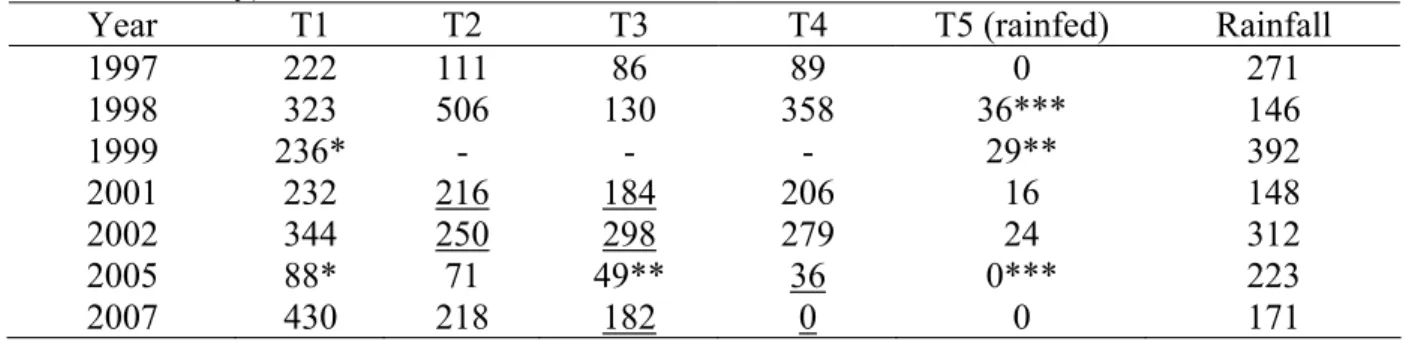
Table 1. Total water application (mm) in different irrigation treatments (Ti) and rainfall (mm)
during the cropping cycle of corn (Samsara variety in 1997-2002 except of 2000 and Pioneer variety in 2007) and durum wheat (Artimond variety in 2005) under conventional tillage and direct seeding into mulch which is underlined (rainfed treatment T5 was irrigated after sowing when necessary)
Year T1 T2 T3 T4 T5 (rainfed) Rainfall
1997 222 111 86 89 0 271 1998 323 506 130 358 36*** 146 1999 236* - - - 29** 392 2001 232 216 184 206 16 148 2002 344 250 298 279 24 312 2005 88* 71 49** 36 0*** 223 2007 430 218 182 0 0 171
* LAI shape parameters, ** LAIst parameter, *** ar parameter calibration
DSM was initiated (for the 2001 season) by sowing oat (October 15th in 2000) which was then destroyed by glyphosat (Rounup®) two weeks prior to corn sowing. The same operation was repeated over the following years except of 2005 where no cover crop was sown before durum wheat cultivation. However there was enough mulch on the soil surface from the precedent crop. The experiments relative to 2003, 2004 and 2006 are out of the scope of this paper because sorghum was sown. For the preparation of the 2007 cropping season, a mixed of oat, vetch and rape was sown in October 2006 in the DSM treatments as cover crop and was destroyed by glyphosat (Rounup®) in April 2007 before corn sowing. In CT plots, at the
end of July disc harrow was used to chop and bury the residues of the precedent crop. At the middle of November, tillage with plough was performed. In DSM plots, the cover crop was sown by a specific seeder namely Semeato®. After destroying the cover crop the same seeder was used to sow the main crop. At the end of November 2004, after two years of a sorghum crop, durum wheat was sown in CT and DSM.
For calibration and validation of the model a database was obtained from experiments on corn in 1997, 1998, 1999, 2001, 2001 and 2007, and on durum wheat in 2005. Fertilizers (N, P, and K) were applied prior to planting and during the season on the basis of soil analysis in such a way that fertilization to be not a limiting factor. To determine the grain yield (GY) and dry matter yield (DM) ten 3 m2 sub-plots were hand harvested. The measured GY and DM variation coefficient (Cv) varies from 6 to 12%.
Table 2. Tillage, sowing and harvest date and N (Kg.ha-1) application for corn (Samsara
variety) in 1997, 1998, 1999, 2001, 2002; for durum wheat (Artimond variety) in 2005 and for corn (Pioneer variety) in 2007 with conventional tillage (CT) and direct seeding into mulch (DSM)
Year treatment Tillage date Sowing date Harvest date N
1997 CT 1/15/1997 5/2/1997 9/15/1997 200 1998 CT 1/10/1998 5/6/1998 9/20/1998 200 1999 CT 1/20/1999 5/26/1999 10/10/1999 150 CT 12/10/2000 5/2/2001 9/10/2001 120 2001 DSM - 5/4/2001 9/10/2001 120 CT 1/6/2002 5/17/2002 9/18/2002 140 2002 DSM - 5/17/2002 9/24/2002 140 CT 9/30/2004 11/17/2004 6/28/2005 149 2005 DSM - 11/30/2004 7/5/2005 149 CT 11/15/2006 4/24/2007 9/28/2007 179 2007 DSM - 4/24/2007 9/28/2007 181
An access tube was installed in each experimental treatment. Soil water reserve (SWR) was monitored once a week using a neutron probe from 0 to 2 m and at 0.1 m depth interval. According to Haverkamp et al. (1984) the accuracy of the measurements ranges from 8 to 10%. A series of mercury tensiometers at 0.1, 0.2, 0.3, 0.4, 0.6, 0.9, 1.0, 1.2, 1.4, 1.6 and 1.8 m depth were located at a distance of 0.4 m from the access tube. They were monitored every morning.
The experimental plan as well as details of the experimental procedure (physiological and meteorological measurements are the same in both field experiments) were similar to that of Olufayo et al. (1996). The LAI measurements were obtained using a Picqhelios apparatus from 1997 to 1999 and using a LI-COR LA1 2000 apparatus for 2001, 2002, 2005 and 2007. According to Mailhol et al. (1997) these two devices give approximately the same LAI values. The Cv of the measured LAI depends on the plant water status and on the phenological stage. It was lower than 15% for corn and durum wheat.
The frequency of irrigation for the full irrigated treatment (without water stress) was derived from Eq.(1):
ETc=R+I- ΔS (1)
, where ETc = crop evapotranspiration, R = rainfall, I =irrigation and ΔS = the change in soil moisture between soil surface and the depth of zero flux plan determined using tensiometers (Vachaud et al. 1978). The soil moisture was measured using a neutron probe. Using Kc from Doorenbos and Kassam (1979) and ETo (reference evapotranspiration) from climatic data, we can calculate ETc. Combining this calculated ETc and ETc from Eq.(1) we program the irrigation as there is not any water stress. According to tensiometers monitoring, there were not any water stress, drainage or capillary rise over the crop season. There was not any runoff too.
Although this article does not focus on the N problem, N amounts are applied in order to fully satisfy plant requirement as soon as a N soil profile was established just before sowing. Two N applications are generally performed, the first one at sowing and the second one 30 to 40 days after sowing (DAS) in the case of corn. For durum wheat, three applications have been done: the first one of 54 Kg/ha on 15 DAS, the second one of 65 Kg/ha on 43 DAS and the third one of 30 Kg/ha on 100 DAS. Due to a problem of equipment availability the usual setup for corn was not respected in 2007. Indeed, the first application of 93 Kg/ha was done in CT but only of 27 Kg/ha in DSM, while the second application was much later than normally
(it was plan to apply one month after sowing) indeed on 70 DAS with 86 Kg/ha for CT and 154 Kg/ha for DSM. With initial N content of 140 Kg/ha in 1.2 m depth for CT vs. 79 Kg/ha for DSM, a lower crop growth potential under DSM than that of CT is predictable despite of a higher second application in DSM. The total N applications are summarized in Table 2.
2.2 Model description 2.2.1 Soil module
The soil module calculates the water balance on a daily (j) time step by means of 3 reservoirs. The basic parameter of this model is the total available water (TAW) expressed in mm/m. It defines as the difference between field capacity (FC) and permanent wilting point (PWP). A shallow reservoir (R1) with a fixed depth, Ps (Ps = 0.1 m) manages evapotranspiration after a supply of water i.e. irrigation or rainfall. The maximum capacity of R1 is:
R1max=TAW Ps (2)
R1 supplies the second reservoir R2 with drainage (d1):
d1(j) = Max{0; R1(j) -R1max} (3)
R2 varies with root growth. The root depth (Pr) can be simulated by:
Pr(j) =Pr(j-1) +Vr (4) , where Vr is the root growth rate (m/day). From sowing, the root system is assumed to be confined to a soil depth of 0.3 m. The duration of this installation is governed by a sum of temperature, Tinst. The value of Tinst can be derived from a zero flux plan monitoring. In some models Vr is linked to the temperature sum. In PILOTE, Vr of the considered day (j) is based on the minimum between a Vr according to thermal conditions (Vrt m/degree.day) and a Vr imposed (Vrs in m/day). The model makes root system to reach the maximum root depth (Rmax) coincide with the LAImax, at this stage the plant mobilizes the available energy to develop the aerial part. However, related to the soil conditions e.g. compaction which affects
Vr, it is relevant in some cases to make the model uses Vrs (case of very compacted soil).
The roots can reach the Rmax which is a plant characteristic where the soil does not physically limit root growth e.g. rock. Initial root depth is set at 0.3 m. After a duration governed by a cumulative temperature threshold (Tinst), rooting evolves from 0.3 m to Rmax (or <Rmax according to thermal conditions).
In the model, first the plant transpiration, Tp and soil evaporation, Es feed from R1 that evolves according to:
R1(j) = R1(j-1)+ R(j) +I(j) – Tp1(j) –Es(j) –d1(j) (5)
, where Tp1 is transpiration which can be calculated as:
Tp1=Cp ETmax (6)
, where Cp is the partitioning coefficient between transpiration and soil evaporation. ETmax can be calculated as:
ETmax=Kc ETo (7)
It is considered that in R1, the plant in competition with soil evaporation can take water without restriction until the R1 becomes empty. Cp is a function of LAI as in Varlet-Grancher et al. (1982):
Cp = 1 - exp (-0.7LAI) (8) , so Es becomes:
Es= (1 - Cp) ETo (9)
, Kc is calculated from LAI according to Allison et al. (1993):
Kc = Kcmax [1-exp(-LAI)] (10) , where Kcmax is the maximum value of the crop coefficient. At each time step, R2 is supplied by drainage, d1 from R1 as:
R2 is growing with θ.Vr, θ (mm/m) being the soil water content of the layer under the root front or the soil humidity of third reservoir, R3. The water balance in R2 can be expressed by: R2(j) = R2(j-1) + θ Vr – Reste(j) + d1(j) – d2(j) (12)
Reste is the complementary water that must be taken by plant from R2 to meet ETmax. When
R1 is empty (θ = PWP) plant takes water only from R2 according to:
Tp2= Kc ETo (13)
The water balance in R3 can be expressed as:
R3(j) = R3(j-1) – θ Vr + d2(j) –D(j) (14)
, where D is drainage from R3 which will be lost completely and it can be calculated according to:
D= Max{0 ; R3max-R3} (15)
, where R3max is:
R3max=TAW[Rmax-Pr(j)] (16)
It is assumed that ET is equal to ETmax as long as R1 contains water and / or the easily usable soil water in R2 is not exhausted. ET calculation in R2 is based on the linear reduction of the
ETmax. The reduction takes effect when the water content of R2 drops below the threshold
value Rs(j) defined by:
Rs(j) = (1- Kr).Pr(j).TAW (17) , where Kr, as proposed by Doorenbos and Kassam (1979), is the ratio between TAW and easily usable soil water. So, transpiration, Tp2 in R2 is calculated by:
Tp2 = Tp Kc ET0 min {1.0, R2(j)/Rs(j)} (18)
As explained in Mailhol et al. (1997), Ps can be set to 10 cm. Soil evaporation is modeled in a very simplified way. But it is not less robust and furthermore it is consistent with more elaborate theories (Hillel, 1980; Campbell, 1985). As long as R1 is not exhausted, evaporation is equal to that imposed by the climate conditions (ETo). In the absence of a crop the R1 is therefore subject to depletion to feed ETo. The R1 protects somewhat the moisture of deeper layers from evaporation producing a mulch effect. Outside the crop season and until a decade after sowing, we consider that evaporation can affect lower layers (below 10 cm) when R1 is exhausted. The R2 contributes in soil evaporation (Es2) according to:
Es2= Ksoil exp [- (1 - θR2)] ETo (19)
, in this empirical formula Ksoil is similar to a resistance of soil to evaporation, being a calibration parameter (close to 0.3 for almost all soils). θR2 is a function equivalent to the full
up level of second reservoir:
θR2= Min [1, R2/TAWR2] (20)
Es2 can be stopped when the humidity in the second reservoir reaches to PWP.
2.2.2 The plant module
LAI is a visible indicator of potential production (quantity of dry matter) of the plant over its
growth. PILOTE simulates the effects of water stress on LAI. We suppose that all factors of production other than water are at their optimum. The formula adopted for the LAI includes the availability of water for the plant through a stress index based on the evapotranspiration calculation provided by the soil module. The LAI increases when the temperature sum (TT(j)) exceeds the temperature sum for emergence Ts. The temperature index is calculated using this expression: TT(j) = k k j = =
∑
1 (Tav-Tb) (21), where Tav is the average daily temperature and Tb is the base temperature. The expression of LAI as in Mailhol et al. (1997) is given by:
( )
(
)
⎥ ⎥ ⎥ ⎥ ⎦ ⎤ ⎢ ⎢ ⎢ ⎢ ⎣ ⎡ − − ⎪ ⎪ ⎭ ⎪⎪ ⎬ ⎫ ⎪ ⎪ ⎩ ⎪⎪ ⎨ ⎧ ⎟ ⎟ ⎟ ⎟ ⎠ ⎞ ⎜ ⎜ ⎜ ⎜ ⎝ ⎛ ⎟ ⎟ ⎟ ⎠ ⎞ ⎜ ⎜ ⎜ ⎝ ⎛ ∑ − − ⎟ ⎟ ⎟ ⎠ ⎞ ⎜ ⎜ ⎜ ⎝ ⎛ ∑ − = = = λ α β α β stress T Ts TT T Ts TT ax LA LAI f j k f j k j Im 1 exp 1 1 1 (22), where LAImax is the maximum LAI value for a crop growing under no limiting conditions (deductible from literature or by measurement), Tf is the temperature sum required to reach
LAImax. This value for most crops, particularly corn, corresponds to flowering. α and β are calibration parameters. α allows model to simulate both growth and senescence. The model provides transition from α=α1 to α=α2=γ when TT exceeds Tf, so that three parameters have
to be calibrated. An automatic calibration procedure exists for this purpose. λ is an empirical parameter reflecting the aversion of the plant to water stress. The practice with the model suggests that a constant value of 1.25 for λ can be adopted for crops such as wheat, corn, soybean, sunflower, and sorghum. The stress index is:
∑
∑
− − = j j j j Tpm Tp stress 10 10 (23), where Tp (=Tp1+Tp2) is the actual transpiration and Tpm is the maximum transpiration. The
model calculates the actual dry matter yield (Ya) as:
Ya = Ym min (1.0, LAIav/LAIopt) (24) , where Ym is potential dry matter obtained without water stress. LAIav is the average LAI calculated during a critical period (which is linked to the effect of water stress on yield), and
LAIopt is the averaged LAI value that should have a non-stressed treatment during the same period in order to obtain the potential yield. It can be derived using the model with stress = 1 in Eq.(22). The critical period can be defined by two temperature threshold corresponding to phonological stages (Ts1, Ts2). LAIav can be calculated according to:
LAIav = 1/Nj
∑
2 1Ts Ts
LAI(j) (25)
, where N is the number of days between Ts1 and Ts2. LAIopt can be calculated with Eq.(25)
by LAI in the treatment without stress. Ym can be obtained by: Ym = RUE maturity
∑
sowing
S(j) I(j) (26)
, where S(j) is the solar radiation (J/m2) from sowing to maturity where the maturity will be driven from maturity temperature sum (Tm, available in the literature or can be measured). I(j) is the fraction of intercepted solar radiation (Moussi and Sacki, 1953):
I(j) = 1- e - k LAI(j) (27)
with:
k = min( 1.0, 1.43 LAI -0.5 ) (28) , where k is the extinction coefficient (Zaffaroni and Schneider, 1989). RUE (g/MJ) is the efficiency of solar radiation interception. It represents the efficiency with which the intercepted radiation is used to produce biomass. The evolution of this parameter over the season is difficult to model because of its dependence (little known) to many factors (Villalobos et al. 1996). Therefore it is better to propose a fixed value for this parameter similar to that at maturity. The approach used here for computing Ym is comparable to that proposed by Villalobos et al. (1996) and Chapman et al. (1993). The RUE value can be calibrated on a full irrigated treatment or derived from literature. In this case, the latter has to
be multiplied by the part of active radiation vs. global radiation (Varlet-Grancher et al. 1982), the value of which is close to 0.5.
2.2.3 Modeling the harvest index (HI) for the grain yield calculation
Grain yield is obtained by multiplying dry matter production by harvest index. HI prediction is not always accurate when modeling the evolution of this factor on the basis of a degree day accumulation. This difficulty is often circumvented by assigning a value often close to the average HIpot, potential harvest index, close to 0.5 for many crops. However this proves satisfactory for the crop whose HI is not sensitive to water stress such as sorghum and sunflower (Mailhol et al. 1997; Cox and Joliffe, 1986) but for other crops such as corn or wheat especially when severe water stress occurs in the process of grain filling it will be different. In the continuity with the approach based on LAI, it is proposed to model HI by: HI =Min [HIpot; (HIpot - ar (LAIst - LAIav )] (29)
, where LAIst being the LAI threshold below which the HI decreases (parameter ar, a
calibration parameter) from its potential value. Note that Eq.(29) offers some flexibility e.g. some crops can have a better HI under a moderate water stress. Such conditions can be simulated when adopting a negative value for ar and an appropriate LAIst. Note that HI is
limited to 0.17 in the model. Indeed, the lowest HI value measured at Lavalette what ever the crop type is about 0.2.
2.3 Modifications to account for mulch impacts
Our modelling approach consists of a simple quantitative description of surface residue effects on the water balance, requiring limited data inputs. That is in contrast with other published more detailed, physically-based mulch models that quantify surface residue impacts on soil water content by solving the balance of energy and water at the soil surface (Bussiere and Cellier (1994); Findeling et al. (2003); Ross et al. (1985)). Parameterization of such models for application to practical problems remains difficult due to the measurement of necessary parameters which are not available for a wide range of conditions. Moreover a large number of these parameters that are related to the physical properties of the mulch layer may change considerably over the season due to decomposition. Xsr, our sole surface residue parameter related to mulch quantity on the soil surface has a direct influence on soil water balance processes. In the present model we did not incorporate other relationships describing mulch impacts to retain model simple and easy to calibrate in different environments. As previously evoked and shown in Khaledian et al. (2006a) for the Lavalette context, the presence of mulch reduces soil evaporation. A first modification of PILOTE to account for soil evaporation reduction due to mulching is proposed. As the shallow reservoir is mainly concerned by this reduction, soil evaporation is calculated according to:
Es =
Xsr
LAI
ET
+
−
1
)
exp(
0ε
(30)In Eq.(28), ε is the extinction coefficient for net radiation in the crop canopy layer (ε ≈0.7 in Eq.(28)), Xsr is an empirical parameter that could be linked to the quantity of mulch on the soil surface (|Xsr|<1; Xsr=0 in CT system). Indeed, this modification is initiated by the approach experimentally deduced by Gusev (2002) where a hyperbolic decrease of Es versus mulch accumulation (MA, Mg/ha) was shown. Es estimation proposed by Eq.(30) is empirical in contrast to that of Perrier and Tuzet (1991) which is physically based but involving parameters which are not easily accessible such as soil resistance or semi empirical approach (Brisson and Perrier, 1991). In the case of existing contrasted mulch treatments, an empirical relationship between Xsr and MA, such as which proposed by Gusev (2002), could be established. That proposed by Gusev (2002) represents Es/Emo vs. mulch quantity (kg/ha),
where Emo is evaporation from a soil without mulch. A comparison with the Scopel approach (Scopel et al. 2004) allows us to give a physical meaning to Xsr. Scopel et al. (2004) used a mulch area index which varies over the crop season (variation not easily predictable), in contrast with PILOTE. Relating to the modifications proposed by Scopel et al. (2004), Es can be calculated as:
Es=ETo exp (-ε LAI) exp (-χ η SR) (31) , where χ= the extinction coefficient for net radiation in the surface residue layer, η = the area covered per unit of residue dry weight (ha/kgDM), SR: the mass of surface residue (expressed as dry matter, DM, per unit area, kg DM/ha). If we compare Eq.(30) and Eq.(31) we find that:
Xsr
+
1
1
= exp (-χ η SR) (32)
, developing the left hand part of Eq.(32):
Xsr
+
1
1
=1-Xsr+Xsr²+…+ (-1)nXsrn+… (|Xsr|<1) (33) , and its right hand part:
exp (-χ η SR) =1- χ η SR+ ! 2 )² (χηSR + ! ) ( n SR n χη +… (|χ η SR|<1) (34) , yields: Xsr≈ χ η SR. For example, if the mulch quantity is 2000 kg/ha, Es/Emo=0.45
(according to Gusev, 2002) or Xsr =0.55 so, the left hand part of Eq.(32) gives
Xsr
+
1
1
≈0.6. In Scopel et al. (2004) with the same quantity of mulch we have SR=2000 kg/ha, (χ= 0.8 and
η= 0.00037; exp (-χ η SR) ≈0.6). The previous developments attest that an experimental
approach could be used to establish a robust link between Xsr and the mulch quantity. For that, the lysimeter method or the zero flux plan method, requiring a TDR probe or a neutron probe and tensiometer monitoring, can be used for soil evaporation assessment. In our study,
Xsr is derived from model calibration by a classical trial and errors approach. The effort of
calibration focuses on a period where its sensitivity on the water balance estimation is the highest. This period is the beginning of the cropping season (from sowing to LAI<3) where
LAI is low and, consequently, soil evaporation is presumed to be high especially for summer
crops (for corn: T3 in 2002).
The second modification concerns root growth rate, Vr, of winter crops which is lower under DSM than under CT. As shown in Fig.1, soil temperature is lower with DSM than CT. This phenomenon is due to soil surface isolation from solar radiation by mulch which retards and limits root development. The impact of this factor on root progression is especially perceptible for crops sown in autumn (or in winter) and for which an adequate and simple Vr has to be proposed. Generally under CT, LAImax and Rmax, are reached at the same time, when all the nutriments allocate to aerial production (grain production mainly). In the case of a winter crop a significant root depth difference can exist between CT and DSM at LAImax for both systems. Consequently, Rmax under DSM is lower than that of CT (Khaledian et al. 2006b). To account for the impact of lower soil temperatures on root progression this second modification was proposed which consisted in the Vr calculation according to:
Vr(j) = min (Vrs,Vrt(j)) (35) In Eq.(35), which is applied for both systems, Vrs is derived from CT system (under no limited water conditions), while Vrt(j) which is related to daily air temperature (m/degree.day) in the case of CT, was calibrated as Rmax and LAImax are reached at the same time. The calibration of empirical relationships between soil temperature under CT (TCT) and DSM
(TDSM) allows an adaptation of Eq.(35) to DSM by correcting Vrt(j) of CT with the TDSM/TCT
0 2 4 6 8 10 12 14 17/2/05 22/2/05 27/2/05 4/3/05 9/3/05 14/3/05 19/3/05 24/3/05 Date S o il t e m p er at u re ° C CT DSM
Fig. 1: Soil temperature at 6 cm in both direct seeding into mulch (DSM) and conventional
tillage (CT) systems in 2005 with durum wheat (Artimond variety).
2.4 Input parameter sensitivity
A sensitivity analysis is useful to indicate which input parameters have the most significant effect on the model output. Particular focus must be set on the measurement or calibration of those parameters. Sensitivity of a certain model output to a given parameter can be defined as the rate of change in the output value resulting from a change of this input parameter while keeping all other parameters constant (Wöhling, 2005). The sensitivity index, SI, proposed by Ng and loomis (1984) was selected for this purpose in the present study. The SI is calculated in (%) by: SI= Δ ×
∑
N= − i Xci Xci Xni N 1 ) ( 100 (36) , where:Xni: the new value of the ith data point with a changed value of the input parameter
Xci: the value of output for the ith point in the control simulation run
N: the number of point
Δ: the absolute change in the input parameter
SI in the given form is a measure of the percentage change in the output from that in the
control simulation resulting from a one percent change in the value of the input parameter. All input parameters were changed by ±25% and ±10% in accordance with the amount of these parameters that we can find for target varieties in our environment.
3. Results and discussions
Calibration and validation are the two necessary steps before model application with confidence, for the varieties and target environment. Results from other environments across the world can be used, reemphasizing the importance of model validation before an application to the definite environment. There are many reports of different crops in different environments around the world. But most of reports provide very little detail on determination of genetic coefficient, and the values which are used. Therefore genetic coefficients for commonly grown varieties of corn and durum wheat are not readily available. Where this information is available, genetic coefficient have generally been determined from only one study. Thus, results of validation may be impaired by poorly derived genetic coefficients, or the conditions between calibration and validation period being different. While the ability of models to simulate the performance of individual crops is very important, it is also desirable to evaluate the performance of cropping systems over a long period.
3.1. Calibration and model validation
The model results were evaluated using two performance criteria: the root mean square error (RMSE) and the coefficient of efficiency (CE) of Nash-Sutcliffe (ASCE, 1993; ASCE: American Society of Civil Engineers). These criteria are used to quantify and to better understand the degree with which the model under/over-estimates.
As explained in Mailhol et al. (1997) the first calibration step consists of determining the shape parameters for the LAI simulation once LAImax is set. The calibration of these shape parameters is done on a full irrigated (non water stressed) treatment by means of the Rosenbrock optimization technique (Rosenbrock, 1960). LAImax values proposed for corn by literature vary from 4 to 5 m²/m², according to plant density and variety. For Samsara, a semi-precocious variety, a LAImax value of 4.5 m²/m² was measured in 1999 on T1 (a non stressed treatment) for a density of 10 plants/m2 with a Tf of 1005 °C (6 °C as Tb) and 1850 °C as Tm. These values were derived from AGPM info (1996; AGPM: l’Association Générale des Producteurs de Maïs) and were verified at Lavalette (Nemeth, 2001). The RUE for corn is set at 1.35 g/MJ, as proposed by literature (Kinitry et al. 1989; Muchow, 1990), after multiplication by 0.5. The Kr parameter was set to 0.6 as the average value for corn (Doorenbos and Kassam, 1979) which is adapted to the potential ET0 rates of the country.
Kcmax was set to 1.2 in CT case as suggested by Doorenbos and Kassam (1979) for corn. Rmax, measured at the end of cropping season (1999 T1) in soil profile was 1.2 m, while the Vrs, obtained by using the zero flux plan monitoring, was Vrs =0.015 m/day and Vrt =
0.001m/degree.day. These values allows the root system to reach at 1.2 m when LAI=LAImax. The maximum yield values (23.1 and 14.2 Mg/ha for DM and GY at 15% of humidity, respectively) were obtained in the full irrigated treatment of 1999 (T1). The two cumulative temperature thresholds Ts1 and Ts2 within which LAI is averaged to correct the potential dry
matter value are 900 and 1600 °C for Samsara, respectively. As proposed in Mailhol et al. (1997; 2004) Ts1 is set at Tf-100 °C while Ts2 corresponds to the vegetative stage measured at
Lavalette: the end of grain filling (pasty grain). As the LAIav value calculated by the model for the rainfed treatment of 1999 is equal to 2.6 m²/m², we suggest to set LAIst at 2.5 m²/m², since HI = HIpot for the rainfed treatment of 1999. As the latter treatment was not subject to a high water stress, the ar parameter of Eq.(29) was calibrated on the rainfed treatment of 1998
where GY was 4.6 Mg/ha (at 15% of humidity) i.e. twice lower than that of 1999. The obtained value is ar =0.12. Previously, it was checked that λ, used in the LAI formulation to
account for water stress condition on LAI, allows a correct simulation of DM for the rainfed treatment in 1998 (9.6 Mg/ha) when setting it to the value obtained in Mailhol et al. (1997; 2004): λ =1.25.
For Pioneer, a late variety, LAImax = 5 m²/m² for a density of 10 plants/m2 is often proposed in literature (Howell et al. 1996). This value was measured on T1 at Lavalette in 2007 with CT. Compared with Samsara, only the temperature thresholds were modified according to variety characteristics. Tm is set at 2000 °C according to that variety (AGPM, 1996) while the measured Tf (cumulative temperature to reach LAImax) was 1050 °C. The temperature threshold Ts2 for Pioneer is set to that of Samsara increased by the difference between Tf
values of these two varieties i.e. Ts2=1650 °C (these values were verified at Lavalette). On
CT, from the yield of sub-plots (Cv= 5%) an average value of 29.4 and 17.4 Mg/ha were obtained for DM and GY, respectively on T1 in 2007, the full irrigated treatment. PILOTE for this treatment simulates 29.2and 17.2 Mg/ha, respectively. DM and GY were satisfactorily simulated by PILOTE: 24.3 vs. 25.2 Mg/ha and 14.3 vs. 14.8 Mg/ha, while the yield on the rainfed treatment is a little under estimated: 11 vs. 12.7 Mg/ha and 4.6 vs. 4.9 Mg/ha.
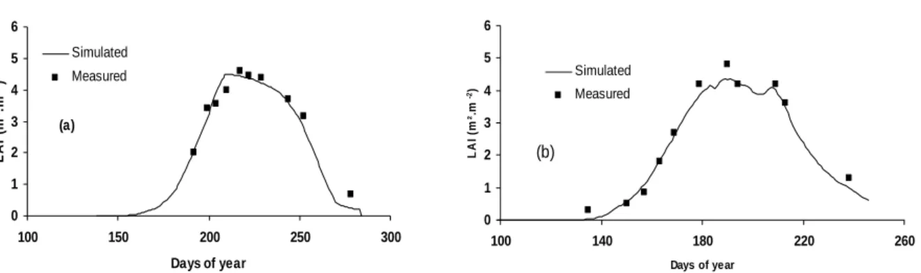
LAI and SWR are satisfactorily simulated for corn and durum wheat in CT. Two examples of LAI and SWR simulations are presented in Fig. 2 and Fig. 3, respectively.
For durum wheat (Artimond variety) the same calibration procedure was used (T1 for the shape parameters). A value of 5 m²/m² is adopted for LAImax value with a plant density of 300 plants/m² (Casals, 1996; Laguette, 1997) with a Tf value of 1200 °C (0 °C as Tb) and 2100 °C as Tm. According to Morgan (1971), the vegetative stage Ts1= Tf-100 (the beginning
of kernel growth stage) and Ts2 = 2000 °C (pasty grain stage). These values were verified at
Lavalette. A RUE value of 1 g/MJ (Casals, 1996, Mailhol et al., 2004) was adopted, Kr = 0.6 and Kcmax = 1.2 were used as suggested by Doorenbos and Kassam (1979) for durum wheat.
Rmax measured at the end of the cropping cycle in a soil profile was 1.5 and 1 m for CT and
DSM, respectively. The stressed treatments T3 and T5 were used for the calibration of LAIst and ar respectively, the HI value for the rainfed treatment was 0.36, being lower than HIpot =
0.5. Rmax decrease in DSM can be explained by DSM impact on root development related to soil temperature. The Vrs, obtained by the zero flux plan monitoring on CT was Vrs = 0.01 m/day, while Vrt is set at 0.0015 m/degree.day in the model. These combined values used in Eq.(35) corrected by the TDSM/TCT ratio, allows Rmax of DSM to be satisfactorily simulated
(Rmax = 1.05 m when LAI ≈ LAImax). Table 1 indicates the treatments involved in model calibration for corn and durum wheat.
0 1 2 3 4 5 6 100 150 200 250 300 Days of year L A I (m ². m -2) Simulated Measured (a) 0 1 2 3 4 5 6 100 140 180 220 260 Days of year L A I (m ². m -2) Simulated Measured (b)
Fig. 2: Leaf area index (LAI) in conventional tillage for corn: (a) Samsara variety in 2002
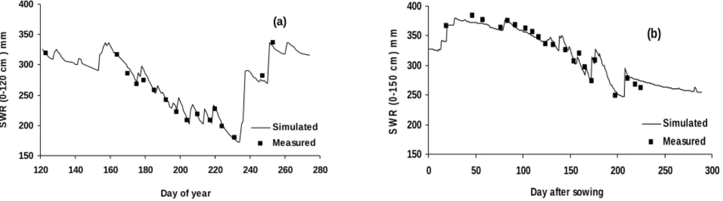
Fig. 3: Soil water reserve (SWR): (a) in 2002 (T1) for corn (Samsara variety; CE=0.98 and
RMSE=6 mm) and (b) in 2005 (T1) for durum wheat (Artimond variety; CE = 0.90 and RMSE
= 13 mm) with conventional tillage system
3.2 The mulch parameter Xsr
In DSM, both soil evaporation and transpiration are reduced. Transpiration diminution results from the presence of a local micro climate emanated by mulch impacts that retains a steady humidity level at the soil surface. This micro climate can limit the convective transfer while reducing the evaporative power of atmosphere. Irrigation rates contribute to this micro climate maintaining more especially for summer crops. It is in agreement with Gusev (2002) who suggested in addition that the mulch thickness must be sufficiently high (5 cm at least) to perceive significant impact on evapotranspiration process. We will see later how to take into account this phenomenon for the soil water balance simulation.
We calibrated PILOTE model with a simple surface residue module in which major mulch effects modify the dynamic of soil evaporation. As previously evoked, our objective is to evaluate the impact of the surface crop residue using a simple modeling approach. Surface residue limits the energy reaching at soil surface, decreasing the first stage of soil evaporation. On the other hand, a layer of surface residue can store an amount of water that evaporates at the first stage. The simulated reduction of soil evaporation by a mulch residue of 1 Mg/ha is about three times larger than the amount of water intercepted and subsequently evaporated from the mulch (Scopel et al. 2004). More especially, under the Mediterranean climate where rainfalls are often high, the ratio between mulch interception and rainfall will be assumed to be negligible, so that we did not take into account mulch interception.
The calibration method used for Xsr in T3 in 2002 yields Xsr =0.5. This value gives correct results for durum wheat too, as further shown.
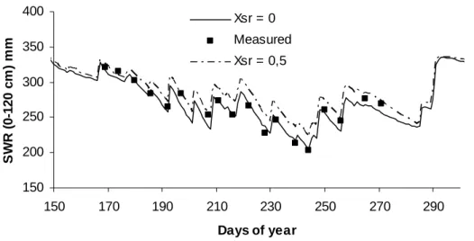
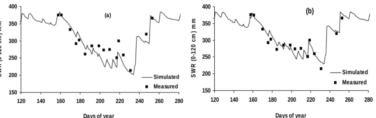
The example proposed in Fig. 4 shows that mulching, imputable to Xsr only (Kcmax being set to 1.2), has a significant impact on the SWR evolution according to PILOTE. That lets us to presume that the potential GY value for corn (Samsara variety, 14.5 Mg/ha) could have been probably reached with a lower water amount than 236 mm (T1) if DSM had been practiced in 1999 where rainfall was particularly high.
Using Xsr = 0.5 and decreasing Kcmax for corn (from 1.2 to 1.1) as previously justified, could improve SWR simulations in the active root zone in DSM. As shown in Fig. 5 for irrigated corn (Samsara variety) and for irrigated durum wheat (Artimond variety), LAI is correctly simulated. 150 200 250 300 350 400 120 140 160 180 200 220 240 260 280 Day of year S W R ( 0 -120 cm ) m m Simulated Measured (a) 150 200 250 300 350 400 0 50 100 150 200 250 300
Day after sowing
S W R (0 -1 5 0 c m ) m m Simulated Measured (b)
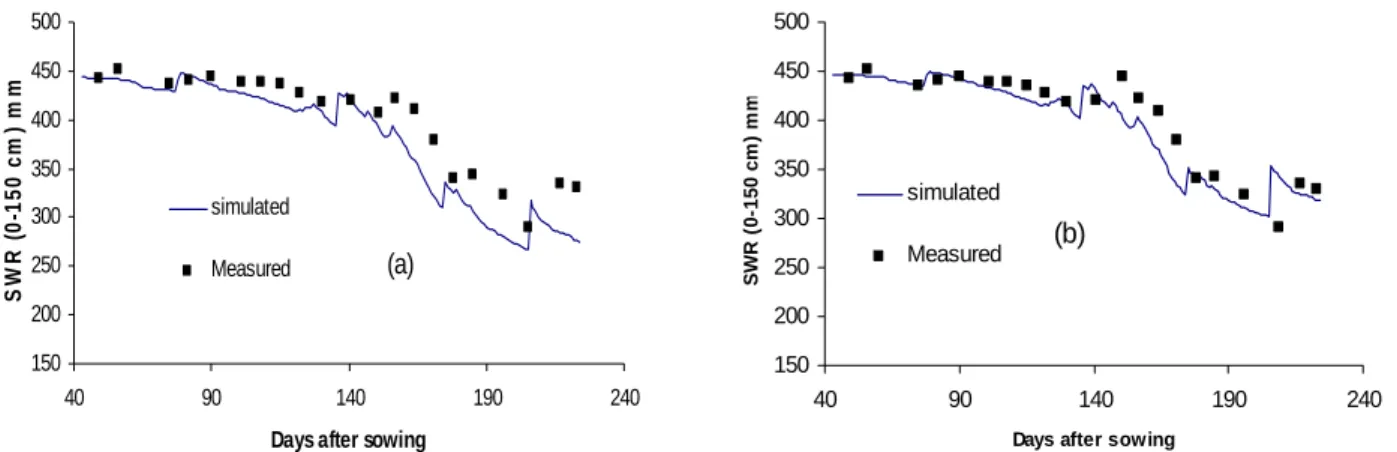
The course of SWR is simulated reasonably well for the DSM treatments (Fig. 6b: CE=0.91,
RMSE=13 mm; Fig. 7b: CE=0.93, RMSE=12 mm; Fig. 8b: CE=0.95, RMSE=11.9 mm) for
corn and durum wheat, while before calibration, some strong discrepancies can be observed for corn (Fig. 6a: CE=0.69, RMSE=25 mm) and for durum wheat (Fig. 7a: CE=0.64,
RMSE=29 mm). For the latter, the modifications in Rmax and Vr considerably improve the SWR simulation. Note that a SWR simulation on 1 m depth (in the active root zone) would
give better results for DSM (CE = 0.96, RMSE = 8 mm). For corn, SWR is correctly simulated in both cropping system after PILOTE adaptation (Fig. 8a with CT: CE=0.98, RMSE=7.3 mm and Fig. 8b with DSM: CE=0.95, RMSE=11.9 mm). Generally, one can say that SWR is satisfactorily simulated by PILOTE for the two corn varieties and durum wheat in CT and in DSM after PILOTE adaptation.
150 200 250 300 350 400 150 170 190 210 230 250 270 290 Days of year S W R (0 -12 0 c m ) m m Xsr = 0 Measured Xsr = 0,5
Fig. 4 Mulching impact on the soil water reserve (SWR) evolution according to PILOTE on
the climatic scenario of 1999 for corn (Samsara variety; T1 in conventional tillage: Xsr = 0;
CE = 0.92, RMSE = 9.0 mm)) 0 1 2 3 4 5 100 150 200 250 300 Days of year LA I ( m ². m -2) Simulated Measured (a) 0 1 2 3 4 0 50 100 150 200 Days of year L A I (m ². m -2) Simulated Measured (b)
Fig. 5: Leaf area index (LAI) in direct seeding into mulch with (a): corn (Samsara variety) in
3.3 Dry matter yield (DM) and grain yield (GY)
Before model adaptation, a disagreement between simulated and observed DM was seen and the simulated results of GY were similar too. This can be related to the over/under-estimation of SWR for treatments where water can be a limiting factor. Indeed, after model adaptation to DSM, improving SWR estimation resulted in better crop yield simulations.
A significant discrepancy is nevertheless noticeable for treatment T3 on DSM in 2007 where the model over estimates the yield (DM: 27.8 vs. 26 Mg/ha, GY: 15.9 vs. 14.1 Mg/ha). The delay of the second N application (70 days after sowing) can be a reasonable explanation of this state of fact, LAI being close to its maximal value at this N application date. Moreover, the low initial N content: 79 vs. 140 kg/ha on CT, (due to N amount initially consumed by cover crop) is another reason of this over estimation by a model that does not consider N as a limiting factor.
Although LAI of the rainfed treatments in CT and DSM for corn in 2007 were not very well simulated (Fig. 9), PILOTE follows the observed tendency regarding the yields. Indeed, in DSM (T4), measured DM and GY are 13 and 6.1 Mg/ha, respectively; while the simulated values are 12.9 and 5.8 Mg/ha i.e. higher than that of simulated in CT (11 and 4.6 Mg/ha). Thanks to soil evaporation reduction under DSM, the soil maintains a humidity level which can delay the water stress occurrence. That is an interesting statement for the regions where sowing irrigation is not usually applied such as in Charente (Ruelle et al. 2003). Indeed, in the perspective of the climatic change (with a spring rainfall decrease), a cropping system avoiding a significant modification of the irrigation scheduling would be probably appreciated by the farmers.
Over the contrasted climatic series for 1997, 1998, 1999, 2001, 2002, 2005, and 2007 the model satisfactorily simulates GY and DM for irrigated and rainfed corn and durum wheat in both DSM and CT systems (Fig. 10). Thus PILOTE, an operative crop model, can be used for water and yield management in CT and DSM systems under Mediterranean climate.
Since it was not the objective of this paper, we did not discuss about the yield difference between CT and DSM systems. One can only refer to published works e.g. Khaledian et al. (2006a; 2006b) showing that for winter crops such as durum wheat, the yields are lower in DSM than in CT, while they are not significantly different for summer crops such as corn.
150 200 250 300 350 400 120 140 160 180 200 220 240 260 280 Days of year S W R (0 -1 2 0 c m ) m m Simulated Measured (a) 150 200 250 300 350 400 120 140 160 180 200 220 240 260 280 Days of year S W R (0 -1 2 0 c m ) m m Simulated Measured (b)
Fig. 6: Soil water reserve (SWR) simulation before (a): (CE=0.69 and RMSE=25 mm) and
after (b): model adaptation (CE=0.91 and RMSE=13 mm) to direct seeding into mulch for corn (Samsara variety) in 2002 (T2)
150 200 250 300 350 400 450 500 40 90 140 190 240
Days after sowing
S W R (0 -1 5 0 c m ) m m simulated Measured (a) 150 200 250 300 350 400 450 500 40 90 140 190 240
Days after sowing
S W R (0 -1 5 0 c m ) m m simulated Measured (b)
Fig.7: Soil water reserve (SWR) simulation before (a): (CE=0.64, RMSE=29 mm) and after
(b): model adaptation (CE=0.93, RMSE=12 mm) to direct seeding into mulch for durum wheat (Artimond variety in 2005, T4)
150 200 250 300 350 400 100 140 180 220 260 Days of year S W R (0 -1 2 0 c m ) m m Simulated Measured (a) 150 200 250 300 350 400 100 150 200 250 Days of year S W R (0 -1 2 0 c m ) m m Simulated Measured (b)
Fig. 8. Soil water reserve (SWR) simulation (a): under conventional tillage (T2; CE = 0.98 and
RMSE = 7.3 mm) and (b): under direct seeding into mulch (T3; CE=0.95 and RMSE=11.9
mm) for corn (Pioneer variety) in 2007
0 1 2 3 4 5 6 100 150 200 250 Days of year LA I ( m ². m -2) Simulated Measured (a) 0 1 2 3 4 5 6 100 150 200 250 Days of year LA I ( m 2 /m 2 ) Simulated Measured (b)
Fig. 9. Leaf area index (LAI) (a): under rainfed conventional tillage (T5) and (b): under
3.4. Sensitivity analysis
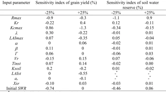
A variation of ±25% was adopted for parameters proper to the model while a variation of ±10% for those measured or derived from literature. For instance, it would not be relevant to make vary a lot a temperature sum characterizing a phonological stage. Indeed, that could either result in a vegetative stage interaction or in a variety change. Table 3 and 4 show variations in GY and SWR vs. variations in input variables using 2007 weather and experiment conditions for corn (Pioneer variety). Simulated GY was most sensitive to FC, high Kcmax,
Tm, HI and RUE. Predicted corn GY is relatively insensitive to the shape parameters of LAI
curve (α, β, γ) and ar. Predicted SWR for corn is most sensitive to Rmax. SWR is low sensitive
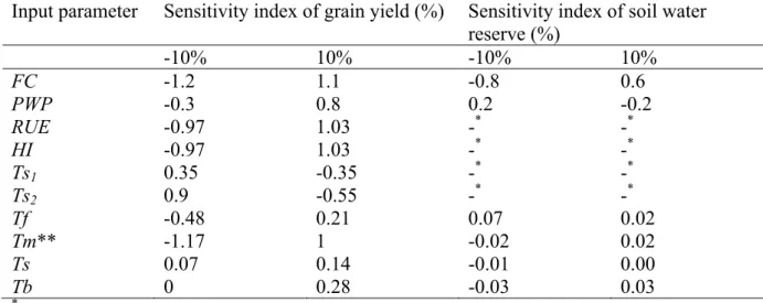
to Xsr. It is relatively insensitive to LAImax and the shape parameters of LAI curve (α, β, γ). Table 5 and 6 show the variations in GY and SWR vs. variations in input variables using 2005 weather and experiment conditions for durum wheat (Artimond variety). Simulated GY is most sensitive to Tb, initial SWR, high FC, high LAImax, high Ts1, low Kcmax, Tf, PWP,
RUE, HI, LAIst, and Ts2. Predicted durum wheat GY is relatively low sensitive to Vr, Ksoil,
LAIst and ar. Predicted SWR for durum wheat is most sensitive to initial SWR and PWP. SWR
is low sensitive to Xsr.
As evoked in Mailhol et al. (1997), initial SWR is a sensitive factor of the model and should be measured as close as possible to the sowing date. From a practical point of view if the initial SWR cannot be measured, it is suitable to start model simulation early in the season i.e. at least one month before sowing date e.g. winter precipitation can fill the SWR in durum wheat case.
Table 3. Input parameter sensitivity for corn (Pioneer variety in 2007) with ±25% changes in
input parameters
Input parameter Sensitivity index of grain yield (%) Sensitivity index of soil water reserve (%) -25% +25% -25% +25% Rmax -0.9 -0.3 -1.1 0.9 Kr -0.22 0.4 0.12 -0.11 Kcmax 0.86 -1.3 -0.34 -0.15 λ 0.30 -0.22 -0.01 0.01 LAImax 0.07 -0.35 0.05 -0.04 α 0 0.06 -0.02 0.01 β 0.11 0 -0.01 0.01 Γ 0.06 0 -0.06 0.03 Vr -0.15 0.15 0.07 -0.06 Tinst 0.07 0.14 -0.02 0.00 Ksoil 0.2 -0.2 0.01 -0.02 LAIst 0 -0.55 -* -* ar 0 -0.1 -* -* Xsr -0.10 0.03 -0.03 0.01 Initial SWR -0.74 0 -0.46 0.06
Table 4. Input parameter sensitivity for corn (Pioneer variety in 2007) with ±10% changes in
input parameters
Input parameter Sensitivity index of grain yield (%) Sensitivity index of soil water reserve (%) -10% 10% -10% 10% FC -1.2 1.1 -0.8 0.6 PWP -0.3 0.8 0.2 -0.2 RUE -0.97 1.03 -* -* HI -0.97 1.03 -* -* Ts1 0.35 -0.35 -* -* Ts2 0.9 -0.55 -* -* Tf -0.48 0.21 0.07 0.02 Tm** -1.17 1 -0.02 0.02 Ts 0.07 0.14 -0.01 0.00 Tb 0 0.28 -0.03 0.03
*not involved in SWR simulation or SI=0
** depending on the importance of water stress during senescence
Table 5. Input parameter sensitivity for durum wheat (Artimond variety in 2005) with ±25%
changes in input parameters
Input parameter Sensitivity index of grain yield (%) Sensitivity index of soil water reserve (%) -25% +25% -25% +25% Rmax 0.11 -0.37 -0.00 1.05 Kr 0.47 -0.74 0.09 -0.08 Kcmax -1.26 0.68 0.16 -0.08 λ -0.16 0.11 0 0 LAImax 0.05 -1.21 0.03 -0.01 α -0.05 0.11 -0.00 0.00 β -0.37 0.37 -0.01 0.00 Γ -0.42 0.47 -0.02 0.01 Vr 0 0 0 0 Tinst 0 -0.13 -0.00 0.01 Ksoil 0 0 -0.02 0.02 LAIst 1.18 -1.32 -* -* ar 0.13 -0.13 -* -* Xsr 0.13 -0.13 -0.01 0.01 Initial SWR -1.85 1.9 -0.4 0.66
Table 6. Input parameter sensitivity for durum wheat (Artimond variety in 2005) with ±10% changes in input parameters
Input parameter Sensitivity index of grain yield (%) Sensitivity index of soil water reserve (%) -10% 10% -10% 10% FC 0.53 -1.18 -0.14 0.07 PWP 1.05 -1.45 -0.27 0.29 RUE -1.05 1.05 -* -* HI -1.18 1.05 -* -* Ts1 0.39 -1.32 -* -* Ts2 1.84 -1.32 -* -* Tf -2.5 1.05 0.02 0.01 Tm** 0.53 0 -0.02 -0.06 Ts 0.13 -0.13 -0.00 0.00 Tb 2.5 1.5 -0.08 -0.08
*not involved in SWR simulation or SI=0
** depending on the importance of water stress during senescence
4. Conclusion
This study attempted to present a simple model, namely PILOTE, for both direct seeding into mulch (DSM) and conventional tillage (CT) systems. The model was calibrated and validated using a 7-year field trial for corn (Samsara and Pioneer varieties) and durum wheat (Artimond variety). The results showed that the model satisfactorily simulates leaf area index, soil water reserve, grain yield and dry matter yield with a minimum coefficient of efficiency of 0.90. This model requires a low number of parameters which most of them can be derived from literatures. Its adaptation to DSM was based on the soil evaporation reduction involving one parameter only in good agreement with the model structure and on the root growth rate for winter crops. PILOTE can be easily calibrated in new environments and for other crops. On the example of corn, the simplicity to adapt the model parameters to a new variety was demonstrated. PILOTE can be used as a reliable tool to provide irrigation programs for a given yield target. We readily acknowledge that PILOTE can be used where water is the only limiting factor which is often the case in Mediterranean countries. A model application on a climatic series would show if yes or not water savings can be obtained under DSM compared with CT for a given yield target. For the evaluation of the environmental benefit that could result from the DSM practice, more complex models than PILOTE have to be used.
References
AGPM info., 1996. AGPM (l’association générale des producteurs de maïs) n°208 July 1996. Ed. AGPM, route de Pau , 64221 France.
ASCE., 1993. American Society of Civil Engineers (ASCE). Task committee on definition of watershed models of the watershed management committee, Irrigation and drainage division: Criteria for evaluation of watershed models. J. of Irrig. and Drain. 119(3), 429-442.
Adekalu, K. O., Fapohunda, H. O., 2006. A numerical model to Predict Crop Yield from Soil-Water Deficit. Biosystems Engineering. 93(3), 359-372.
Allen, R. G., Pereira, L. S., Raes D., Smith, M., 1998. Crop evapotranspiration: Guidelines for computing crop water requirements. Irrig and Drain. Paper 56 FAO, Rome. 300 pp. Allison, B.E., Fechter, J., Leucht, A., Sivakumar, M.V.K., 1993. The use of the
Irrigation and Drainage. 2nd Workshop on Crop Water Models. The Hague, the Netherlands 1993. Session III. p. 17.
Andalesa, A. A., Batchelor, W. D., Anderson, C. E., Farnham, D. E., Whigham, D. K., 2000. Incorporating tillage effects into a soybean model. Agricultural system. 66, 69-98. Braud, I., 1998. Numerical discretisation of the version of SiSPAT model taking into account
mulch horizon. LTHE (CNRS UMR 5564, IMPG UJF) Grenoble.
Brisson, N., Perrier, A., 1991. A semi-empirical model of bare soil evaporation for crop simulation models. Water Resour. Res. 27(1), 719-727.
Bussiere, F., Cellier, P., 1994. Modification of the soil temperature and water content regimes by a crop residue mulch: experiment and modelling, Agric. For. Meteorol. 68(2), 1-28.
Campbell, G. S., 1985. Soil physics with basic. Transport models for soil-plant systems. Elsevier, Amsterdam. 150 pp.
Casals, M-L., 1996. Introduction des mecanismes de resistance a la secheresse dans un modele dynamique de croissance et de developpement, du ble dur. Thèse de doctorat INRA. 93 pp.
Cavero, J., Farre, I., Debaeke, P., Faci, J-M., 2000. Simulation of maize yield under water stress with the EPICphase and CROPWAT models. Agron. J. 92, 679-690.
Chapman, S.C., Hammer, G.L., Meinke, H., 1993. A sunflower simulation model: I. Model development. Agron. J. 85, 725-735.
Cox, W.J., Jolliff, G.D., 1986. Growth and yield of sunflower and soybean under soil water deficits. Agron. J. 78, 226-230.
Doorenbos, J., Kassam, A. H., 1979. Yield response to water , Irrig. and Drain. Paper N° 33, FAO, Rome (Italy), 235 pp.
Enrique, G. S., Braud, I., Jean-Louis, T., Michel, V., Pierre, B., Jean-Christophe, C., 1999. Modelling heat and water exchanges of fallow land covered with plant-residue mulch. Agricultural and Forest Meteorology. 97(3), 151-169.
Fischer R. A., Santiveri F., Vidal I. R., 2002. Crop rotation, tillage and crop residue management for wheat and maize in the sub-humid tropical highlands: I. Wheat and legume performance, Field Crops Res. 79, 107-122.
Findeling, A., 2001. Etude et modélisation de certains effets du semis direct avec paillis de résidus sur les bilans hydriques, thermique et azoté d’une culture de maïs pluvial au Mexique. Thèse de doctorat ENGREF. 355 pp.
Findeling, A., Ruy S., Scopel E., 2003. Modeling the effects of a partial residue mulch on runoff using a physically based approach, J. Hydrol. 275, 49-66.
Gusev, E., Busarova, O, Yasitskiy, S., 1993. Impact of a mulch layer composed by organic remains on the soil the thermical conductions following snowmelt. Journal of Hydrolo. Hydromech. 41(1), 15-28.
Gusev, E., 2002. The technique of assessment of impact of mulching soil by plant remains on formation of water regime and yield of agricultural ecosystems. Water Problem Institute, Russian Academy of Sciences, In third international conference on water resources and environmental research, Dresden (Germany) 22-25 July 2002: 168-172. Haverkamp, R., Vauclin, M., Vachaud, G., 1984. Error analysis in estimating soil water
content from neutron probe measurements: 1. Local standpoint. Soil Sci. 137 (2), 78-90. Hillel, D., 1980. Fundamentals of soil physics. Academic press, New York. 413 pp.
Howell, T.A., Evert, S.R., Tolk, J.A., Schneider, A.D., Steiner, J.L., 1996. Evapotranspiration of corn Southern High Plains, ASE, Proceeding of ASE, San Antonio TX, 3-7 November 1996. 158-166.
Jamieson, P. D., Porter, J. R., Goudriaan, J., Ritchie, J. T., van Keulen, H., and Stol, W., 1998. A comparison of the models AFRCWHEAT2, CERES-Wheat, Sirius, SUCROS2
and SWHEAT with measurements from wheat grown under drought. Field Crops Research. 55(1-2), 23-44.
Jongschaap, R. E. E., 2007. Sensitivity of a crop growth simulation model to variation in LAI and canopy nitrogen used for run-time calibration. Ecological Modelling. 200(1-2), 89-98.
Khaledian, M. R., Ruelle P., Mailhol J.C., Delage L., Rosique P., 2006a. Sustainability of direct seeding versus conventional tillage, 14th International Soil Conservation Organization Conference, Water Management and Soil Conservation in Semi-Arid Environment (ISCO2006), Marrakech, Morocco, 14-19 May 2006.
Khaledian, M. R., Ruelle P., Mailhol J.C., Delage L., Rosique P., 2006b. The long-term impacts of direct seeding into mulch in the south of France, World Congress: Agricultural Engineering for a Better World, Bonn, Germany, 3-7 September 2006. Kinitry, J.R., Jones, C.A., O’Toole J.C., Blanchet , R., Cabelgenne M., Planel, D.A., 1989.
Radiation use efficiency in biomass accumulation prior to grain filling for few grain crops specie. Field crop research. 20, 51-64.
Laguette, S., 1997. Utilisation des données NOAA-AVHRR pour le suivi du blé à l’échelle de l’Europe. Thèse de doctorat ENGREF. 167 pp.
Lamarca, C. C., 1996. Stubble Over the Soil: The Vital Role of Plant Residue in Soil Management to Improve Soil Quality. American Society of Agronomy, Madison, Wisconsin. 245 pp.
Licht, M. A., Al-Kaisi, M., 2005. Strip-tillage effect on seedbed soil temperature and other soil physical properties. Soil and Tillage Research. 80(1-2), 233-249.
Mailhol, J.C., Olufayo A., A., Ruelle, P., 1997. Sorghum and sunflower evapotranspiration and yield from simulated leaf area index. Agric. Water Manag. 35, 167-182.
Mailhol, J.C., Zaïri A., Slatni A., Ben Nouma, B., El Amami, H., 2004. Analysis of irrigation systems and irrigation strategies for durum wheat in Tunisia. Agric. Water Manag. 70, 19-37.
Morgan, J.M., 1971. The death of spikelet in wheat due to deficits. Aust. J. Exp. Agric. Anim. Husb. 43, 968–972.
Mousi, M., Sacki, T., 1953. Über den Lihtfaktor in den Pflanzengesellschaften und seine Bedeutung fur die Stoffproduktion. Jpn. T. Bot. 14, 22-52.
Muchow, R. C., 1990. Effect of high temperature on the rate and duration of grain growth in field-grown Sorghum bicolour (L.) Moench. Aust. J. Agric. Res. 41, 329-337.
Nemeth, I., 2001. Devenir de l’azote sous irrigation gravitaire. Application au cas d’un perimètre irrigué au Mexique. Thèse de doctorat Univ. Montpellier II , 210 pp.
Ng, N., Loomis, R. S., 1984. Simulation of growth and yield for the potato crop. Simulation monographs. Pudoc (Centre for Agricultural Publishing and Documentation, P.O. Box 4, 6700 AA Wageningen), 147 pp.
Olufayo, A., Baldy, C., Ruelle, P., 1996. Sorghum yield, water use and canopy temperatures at different levels of irrigation. Agric. Water Manag. 30, 77-9
Perrier, A., Tuzet. A., 1991. Land surface processes: description, theoretical approaches and Physical laws under laying their measurements. In: Land Surface Evaporation. Measurement and parametrization, T.J.Schmugge et J.-C. André (Eds). Springer-Verlag, New York, pp. 145-155.
Rhoton, F., 2000. Influence of time on soil response to no-till practices. Soil Sci Soc. of American Journ. 64, 700-709.
Rosenbrock, H., 1960. An automatic method for finding the greatest or the least value of a function. Comput. J. 3, 175-184.
Ross, P.J., Williams, J., McCown, R.L., 1985. Soil temperature and the energy balance of vegetative mulch in the semi-arid tropics: II. Dynamic analysis of the total energy balance. Aust. J. Soil Res. 23, 515-532.
Ruelle, P., Mailhol, J.C., Quinones, H., Granier, J., 2003. Using NIWASAVE to simulate impacts of irrigation heterogeneity on yield and nitrate leaching when using a travelling rain gun system in a shallow soil context in Charente (France), Agric. Water Manag. 63, 15-35.
Scopel, E., 1994. Le semis direct avec paillis de résidus dans la région de V. Carranza au Mexique: Intérêt de cette technique pour améliorer l’alimentation hydrique du mais pluvial en zones à pluviométrie irrégulière. Thèse de doctorat, Institut Agronomique de Paris Grignon, 334 pp.
Scopel, E., Macena, F., Corbeels, M., Affholder, F., Maraux, F., 2004. Modelling crop residue mulching effects on water use and production of maize under semi-arid and humid tropical conditions. Agronomie. 24, 1-13.
Shpiler, L., Blum, A., 1991. Heat tolerance to yield and its components in different wheat cultivars. Euphytica. 51, 257-263.
Timsina, J., Humphreys, E., 2003. Performance and application of CERES and SWAGMAN Destiny models for rice-wheat cropping systems in Asia and Australia: a review. CSIRO Land and Water. Griffith. Technical Report 16/03. 53 pp.
Unger, P., Parcker, J., 1976. Evaporation reduction from soil with wheat, sorghum and cotton residue. Soil Sci Soc of Am. Journ. 40, 63-89.
Vachaud, G., Dancette, C., Sonko, S. Thony, J. L., 1978. Méthode de caractérisation hydrodynamique in situ d’un sol non saturé: Application à deux types de sols au Sénégal en vue de la détermination des termes du bilan hydrique. Ann. Agron. 29, l-36. Varlet-Grancher, C., Bonhomme, R., Chartier, M., Artis, P., 1982. Efficience de la
consommation de I’tnergie solaire par un couvert vCgCta1. Oecol Plant 3, 3-26.
Villalobos, F.J., Hall, A.J., Ritchie, J.T., Orgaz, F., 1996. OILCROP-SUN: A development. growth, and yield model of the sunflower crop. Agron. J. 88, 403-415.
Weill, A. N., McKyes, E., Mehuys, G. R., 1989. Agronomic and economic feasibility of growing corn (Zea mays L.) with different levels of tillage and dairy manure in Quebec. Soil Tillage Res. 14(4), 311-325.
Wöhling, T., 2005. Physically based modeling of furrow irrigation systems during a growing season. Dissertation, Dresden University. 209 pp.
Zaffaroni, E., Schneiter, A. A., 1989. Water-use efficiency and light interception of semi-dwarf and standardheight sunflower hybrids grown in different row arrangements. Agron. J. 81, 831-886.