HAL Id: hal-00944775
https://hal.archives-ouvertes.fr/hal-00944775
Submitted on 11 Feb 2014
HAL is a multi-disciplinary open access
archive for the deposit and dissemination of sci-entific research documents, whether they are pub-lished or not. The documents may come from teaching and research institutions in France or abroad, or from public or private research centers.
L’archive ouverte pluridisciplinaire HAL, est destinée au dépôt et à la diffusion de documents scientifiques de niveau recherche, publiés ou non, émanant des établissements d’enseignement et de recherche français ou étrangers, des laboratoires publics ou privés.
Automatic Parameter Setting of Random Decrement
Technique for the Estimation of Building Modal
Parameters
Fatima Nasser, Zhong-Yang Li, Nadine Martin, Philippe Guegen
To cite this version:
Fatima Nasser, Zhong-Yang Li, Nadine Martin, Philippe Guegen. Automatic Parameter Setting of Random Decrement Technique for the Estimation of Building Modal Parameters. International Con-ference Surveillance 7, Oct 2013, Troyes, France. 13 p. �hal-00944775�
Automatic Parameter Setting of Random Decrement
Technique for the Estimation of Building Modal Parameters
Fatima Nasser
1, Zhongyang Li
1, Nadine Martin
1and Philippe Gueguen
21
Gipsa-lab, Departement Images Signal
BP 46 – 961 F-38402 Saint Martin d’Heres, France
{fatima.nasser, zhong-yang.li, nadine.martin}@gipsa-lab.grenoble-inp.fr
2
ISTerre, Univ. Grenoble /CNRS/IFSTTAR
BP 53, 38041 Grenoble cedex 9, France
Abstract
This paper examines the use of the Random Decrement Technique (RDT) for the estimation of building modal parameters, in particular the natural frequency and the damping ratio. It focuses on establishing the processing parameters one must specify to use the technique to its best advantage. This work is motivated by the high influence of these parameters on the RDT quality. Despite the widespread use of the RDT and the enormous effort for understanding the choice of its parameters, no work has been done on how to automate this selection. From this point, this paper comes out with a proposition of an automatic procedure to guide up the choice of these parameters. The results of this paper, on simulated and real-world ambient vibrations, indicate that the proposed automatic setting procedure of the different parameters of the RDT has opened the way to more reliable results and much credible estimation of the modal parameters.
1 Introduction
The RDT was introduced by Cole during the late 1960s [1], for the analysis of response measurements only. The principle of this technique is to estimate Random Decrement Signatures (RDSs) by averaging time segments of the measured structural responses. These segments are selected under certain conditions known as triggering conditions. The modal parameters of the structure can be then extracted from the RDSs using methods developed to extract these parameters from free decays.
Since its development, the theory behind this technique has been widely investigated [2, 3, 4, 5], with a significant concentration on the parameters contributing to the performance of the RDT. For example, studying the filtering effect [6], exploring the difficulties of choosing the triggering levels for a given triggering condition [3], and discussing the number of segments needed to yield reliable estimates [7], however none of them had addressed a way of setting these parameters automatically. This paper responds to this deficiency by proposing an automatic procedure for setting the RDT related parameters.
The natural starting point is the definition and the estimation of RDS which is shown in section 2. The contribution of this work is discussed in section 3. Sections 4 and 5 explore respectively an overview of the proposed algorithm and a detailed explanation of its steps. The obtained results are examined in section 6 over simulated and real-world ambient vibration signals. Section 7 draws the conclusions of this paper.
2 RDS definition and estimation
The RDSs DY(τ)are defined as the mean value E
[ ]
.. of a process Y(t)given some triggering conditions) (t
Y
T at an actual time t,
DY(τ)=E
[
Y(t+τ)TY(t)]
, (1)For a time series, the RDSs can be estimated unbiased as an empirical mean ˆ ( ) 1 ( ) ( ) 1 i N i i y Y y t T t N D ∑ = + = τ τ , (2)
The triggering condition presents the basic requirement for the initial condition of the time segments in the averaging process at the time lag τ =0. All the different triggering conditions used can be considered as specific formulation of the applied general triggering condition, GA
t Y T()
TYGA(t) =
{
a1≤Y(t)>a2,b1≤Y(t)>b2}
. (3) where a1,a2, b1and b2 are the triggering levels.The most frequently used triggering conditions are level crossing, TL
{
Y t a}
t Y() = ()= , positive point,{
1 2}
) ( a Y(t) a TP t Y = ≤ > , local extrema, T () ={
a1≤Y(t)>a2,Y(t)=0}
E tY , and zero-up crossing,
{
() 2, ( ) 0}
)
( = Y t =a Y t >
TZ t
Y . The number of triggering points controls the estimation time and the accuracy of
the estimates [4].
3 The contribution of this work
When firstly introduced by Cole [1], RDT was intended to extract one vibration mode out of the narrow-band filtered response measurement, called the RDS. Accordingly, a filtering process is required as a first step in a multi-mode context.
Since filtering is the first step to condition the data for analysis in the RDT; therefore, it should be carried out with high precision. To achieve that and to initialize this process, we propose to set the filter parameters from a spectrum of the process Y(t)as described in Section 5.
The second step consists of segmenting the filter output of each mode in order then to average the segments and to retrieve an approximated system response with a correct modal parameters. For this step, we compare the different triggering conditions proposed in the literature, such as [5]. After averaging, the method provides a signature of a single-degree-of-freedom system for each mode. From these signatures, the modal parameters of each mode can be estimated. To evaluate the reliability of the estimation, we tested our proposed method over real-world and simulated ambient vibration signals.
This paper has greatly shown that when the first step of the RDT is well done, i.e. the filtering process is very well performed; the other parameters, like the segment length and the different types of triggering conditions, will have less effect on the RDS estimation and the modal parameter extraction.
4 Overview of the proposed algorithm
In the proposed algorithm, the frequency bands of the signal components were detected using Welch’s spectral estimator. The data-driven interpretation of the spectrum is carried out over each frequency sample to determine whether the frequency corresponds to a mode or noise only. The noise spectrum, which has to be estimated as the spectral content corresponding to the additive noise, is extracted using a multi-pass filtering method [8] [9]. Based on the result of the noise spectrum estimation, a peak detection method is applied with a given false alarm probability to distinguish the spectral content of interest from the noise spectrum [10]. In this paper, the spectral peaks are detected by a Neyman-Pearson hypothesis test that requires the choice of a false alarm probability and the estimation of the noise spectrum.
The peak detection method estimates q=1...Q peaks that we associate with the modes of the signal. For setting the filter bandwidth of each peak we propose to estimate it from the bandwidth of these detected peaks. The method is simply based on localizing the minima of the q=1...Q peaks, [L (left minimum), q
q
R (right minimum)].
Followed by a filtering process, the detected peaks and their related minima are connected in sequence to form the input of the filter. Accordingly, a filtered signal will be in use to estimate the RDS of each mode, which will be in turn used for modal parameters extraction. In this way, the filtering process is automatically achieved with paying high attention to its parameters, yielding a good RDS and modal parameter estimations.
5 Algorithm details
In this section, we describe the main steps of the algorithm proposed. Figure 1 shows the entire estimation process that can be summed up in 4 steps. Concerning the need to recognize the modal parameters
of all components of the signal, the algorithm starts by calculating the spectrum Sy
[ ]
f of signaly[ ]
t using a Hamming window ofL
t points where L is chosen as tres dB t
f
Fs
b
L
=
−3*
. (4)where Fs is the sampling frequency,
b
−3dB and fres are the -3 dB bandwidth of the main lobe of the spectral window (b
− dB3=
1
.
3
for Hamming) in frequency bins and Hz respectively. Instead of fixing the window length, we chose to fix the bandwidth fres, regarded as the frequency resolution of the analysis, according to a priori physical knowledge of the signal.Each maximum of the spectrum corresponds to two categories, either the noise e
[ ]
t or the signal of interests[ ]
t . As in [9], we use a peak detection method to classify all of the maxima according to the two categories of spectral contents. The principle is to build a hypothesis test based on these two hypotheses.The algorithm requires the following parameters: Qis the assumed number of the detected peaks; Lt is
the time window length of the Welch estimator; Lf is the frequency window length of the multipass filter;
γ
PFA is the false alarm probability needed for the noise spectrum estimation; Pis the number of passes;
d
PFA is the false alarm probability. These parameters and steps of the algorithm are detailed in Section 5. The great advantage of the proposed algorithm is that the peak detection strategy is adjusted to the data and the statistical properties of the spectrum estimator. Therefore, heavy manual configurations are avoided. With the noise spectrum γˆ
[ ]
f estimated from the local spectrum itself using a multipass filtering method, the calculation of the detection threshold depends on the false alarm probability chosen by the user. The spectral contents of interest hereby detected are referred to as “peaks”, which are essential to the bandwidth estimation, and thus filtering procedure which is an essential step for the RDT.Figure 1: Flow chart of the global algorithm. Given the input signaly
[ ]
t , the algorithm provides the number of peaks Q, the bandwidth and the segment length estimations, using the parameters Lf,PFAγ,d
PFA , MSEenv,MSEf, and the filtered signal Yq
[ ]
t5.1 Welch spectral estimator method
The Welch spectral estimator method must firstly be computed. The estimation of the power spectrum is carried out by dividing the time signal into successive blocks, calculating the periodogram for each block, and averaging the periodograms of the signal blocks.
Let ym denotes the mthblock of the signal y, and let M
(
∀M∈Ζ)
denote the number of blocks.Then the PSD estimate, Sy
[ ]
f , is given by[ ]
{
m f}
m M m f m y DFT y Y w M f S 2 2 1 0 ) ( ) ( 1 − ∆ = = ∑ = (5)Where the notation
{}
m
.
is the time averaging across blocks of data indexed by m.0 2000 4000 6000 8000 10000 12000 14000 16000 -0.03 -0.02 -0.01 0 0.01 0.02 0.03 Signal Points A m pl it ude 0 20 40 60 80 100 -250 -200 -150 -100 -50 0
Welch spectral estimator
Frequency (Hz) P ow e r di s tr ibut ion ( dB )
Figure 2: A simulated ambient vibration signal of 16000 points, sampled at 200 Hz (left), and its PSD estimated by the Welch’s method with a hamming window of 867 points (right)
The PSD estimated by the Welch’s method is illustrated in Figure 2 (right).
On the calculated spectrum, the Neyman-Pearson hypothesis test described in Section 5.1 is applied. The analysis based on such a test consists of two major steps. The first step is to estimate the noise spectrum. The estimation is done by a multi-pass filtering technique, as described in Section 5.2. The second step is to detect the peaks based on the noise spectrum, using a data-driven peak detection method, as described in Section 5.3. Both of these steps are based on the Neyman-Pearson hypothesis test as described in 5.1. The detected peaks are finally connected by the bandwidth estimation method proposed in section 5.4.
5.2 Hypothesis test for peak detection and removal
The spectrum of a general noisy observation y ,...,
[ ] [ ]
1 yN can be expressed as[ ] [ ] [ ]
f S f S fSy = s + e (6)
where Ss
[ ]
f and Se[ ]
f are respectively the local spectrum of the pure signal s ,...,[ ] [ ]
1 sN and of the additivenoise e ,...,
[ ] [ ]
1 eN , with N being the length of the signal. We define here two types of spectral contents as two hypothesis respectively,[ ] [ ]
[ ] [ ] [ ]
f S f S f S H f S f S H e s y e y + = = : , : 1 0 (7)When
H
1 is not known, as is the case in this paper, we can apply a Neyman-Pearson lemma [11], with ). ) ( ( ProbT f H0 PFA= >λ (8)where λis the test threshold, PFAis the false-alarm probability. The test result is given by
. ) ( 1 0 λ < > H H f T (9)
In this test, the threshold λ is calculated from an a-priori chosen PFAand using the statistical properties of the spectrum estimator. For Welch’s method without overlapping between the blocks, the random variable
[ ]
[ ]
f S f S f T e y 2 )( = can be regarded as having a
χ
2M2 distribution [10] ,of degree of liberty 2M if the noise e[ ]
n is Gaussian. 2 2)
(
f
MT
≈
χ
(10)Combining (8) and (10), the detection threshold λ can be determined by
. ) ( ) ( 2 2 0 ) ( x dx p x dx p PFA M H f T
∫
∫
+∞ +∞ = = λ χ λ (11)Then the test hypothesis (8) becomes
[ ]
. ) ( 1 0 f S H H f T >< λ× e (12)From (12), the test depends on the a-priori choice of the false-alarm probability PFAand the estimation of the unknown noise spectrum Se
[ ]
f .In the proposed algorithm, the test is used twice: in the noise spectrum estimation and in the peak detection. For the noise spectrum estimation described in Section 5.2, it is necessary to remove peaks using this hypothesis test with a false-alarm probability referred as PFAγ. For the peak detection in Section 5.3, the test is applied using another value, referred to PFAd.
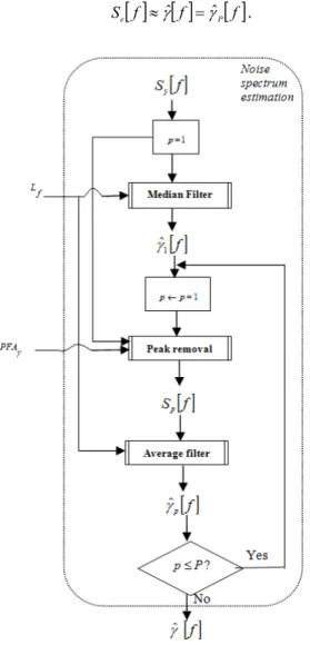
5.3 Estimation of the noise spectrum
We propose to approximate the unknown noise spectrum Se
[ ]
f as γˆ[ ]
f through an iterative process; namely, the multipass filtering that was developed in [8] [9]. The entire procedure of multipass filtering can be summarized by Fig. 3. The first pass in a Lf-point median filter,[ ]
{ }
[ ]
' 1 ˆ f =FILTERmedian S f γ , with 2 ) 1 ( ,..., 2 ) 1 ( '= − f − + Lf + f L f f , (13)where γˆ1
[ ]
f is the estimation result of the first pass. Lfis an odd number specifying the length of the slidingfilter window. Normally this length is
res main f res main
f
Fs
b
L
f
Fs
b
4
3
≤
≤
(14)with
b
main the normalized bandwidth between the two zeros of the main lobe of the chosen window function (For Hamming windowb
main=
4
). The estimated noise spectrum is refined in the following P−1passes. Each pass has two steps, the peaks corresponding to spectrum Sy[ ]
f are removed by applying the hypothesis test described in the previous section, with a false-alarm probability PFAγ and the previously estimated noise spectrum γˆp 1−[ ]
f . All peaks verifying H1are removed from the local spectrum to yield its peak-free part[ ]
fSp . The second step smooths the remaining part Sp
[ ]
f by an average filter with a gliding window of M points. The estimated noise spectrum is upgraded by the filter output. The final noise spectrum γˆ[ ]
f estimation is the output after Ppasses,[ ] [ ] [ ]
f f fSe ≈γˆ =γˆP . (15)
Figure 3: Decomposition of the block noise specterum estimation in Figure 1, done by multipass filtering with Ppasses. Based on the local spectrum Sy
[ ]
f , the noise spectrum is finally estimated as γˆ[ ]
f using asliding window Lf frequency samples and the false alarm probability PFAγ.
5.4 Peak detection
Based on the estimated noise spectrum, another Neyman-Pearson test is applied to identify the peaks verifyingH1. For each frequency indexf , a hypothesis test is carried out using the test statistic as explained
in section 5.1.
[ ]
ˆ[ ]
. 1 0 f H H f Sy <> λ×γ (16)An example of the peak detection is shown in Figure 4. The peaks are defined as the vertex of the bell shapes above the detection threshold λ ˆ×γ
[ ]
f . Each peak is represented by its frequency fq.Figure 4: Peak detection on local spectra of the signal of Figure 2, with
PFA
γ=
10
−4 andPFA
d=
10
−3. (∆ ) Detected peaks over the threshold λ ˆ×γ[ ]
f calculated with PFAγ =10−4. Local maxima below the λ ˆ×γ[ ]
fare treated as noise.
5.5 Bandwidth estimation
For each detected peak q=1...Q ,we propose to localize its left and right minima, denoted as
q
L and
R
q respectively. Then a symmetry test is carried out for all the peaks of neither lowest nor highest frequency ranges. The test consists of accepting the symmetry of either L or q R under a condition that no qother mode is included in the symmetry range.
However, for the lowest and the highest frequency ranges peaks, the R and q L will be used q
respectively as the bandwidth range for the filtering process as shown in Table 1.
Freq. range Filter Bandwidth
Lowest freq. LPF
[ ]
RqHighest freq. HPF
[ ]
LqNeither lowest nor
highest freq. BPF
[
fq −min(fq −Lq,Rq − fq),fq +min(fq −Lq,Rq − fq)]
Table 1: Filter bandwidth range of the detected modes with L and q R the localized left and right minima q
respectively, and f the frequency of the detected peak q
5.6 Modal parameter estimation
Given that the RDS, DˆY(τ), decays as e−ξ2πfnτ, estimates of the damping ratios, ξ, are obtained by a
Least Square Fit (LSF) of the envelope. The method takes care of the smallest error between the envelope and the fitted function. The equation for this method is
[
]
2 1 2 ) ( 1 ∑ = − − = N i i n f i Y e D N LSF τ ξ π τ (17)where τiare time instants corresponding to the extrema of the RDS.
However, for the estimates of the modal frequencies, the zero crossing frequency estimation is used. This method is widely used because of its simplicity [12], it is based on a zero crossing scheme. The frequency of a signal is estimated quite simply as the zero-crossing rate.
(
)
∑ = − − = N i i i N f 12 0, 0, 1 1 1 τ τ (18)where
τ
0,iis the ith zero crossing of the RDS.6 Performance analysis
To test the relevancy of the RDT over the proposed method, many different simulated and real-world ambient vibration signals were used, here we present two simulated and one real-world data.
In this paper MATLAB programming is used for implementation of proposed algorithm. The Butterworth filter has been used to filter the signals under study. It was supplied with the desired passband
p
f , and stopband cutoff frequencies f , the allowable passband ripple s R , and the minimum stopband p
attenuation R . Then it provides the filter order and the normalized bandwidth s W of such a filter. n
6.1 Application on simulated signals
The simulated signals are obtained from a continuous physical modeling of a building defined as an equivalent Timoshenko beam with a simple 1D linear lumped mass model. At each level of the building, an ambient vibration is generated as the dynamic response of this model, which is excited by a ground solicitation assumed to be white and Gaussian [13].
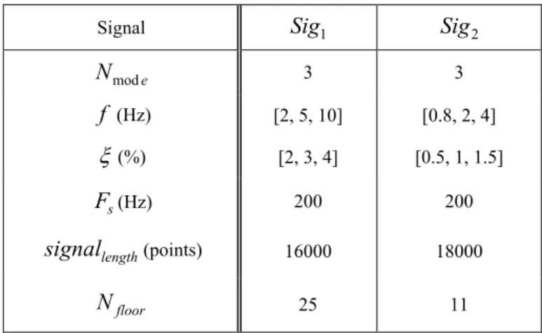
Two signals of different configurations were simulated as is shown in Table 2.
Signal Sig1 Sig2
e Nmod 3 3 f (Hz) [2, 5, 10] [0.8, 2, 4] ξ(%) [2, 3, 4] [0.5, 1, 1.5] s F (Hz) 200 200 length signal (points) 16000 18000 floor N 25 11
Table 2: Two simulated signals (Sig ,1 Sig ), with different configurations of 2 Nmode being the number of modes, f and ξ the modal frequencies and the damping ratios of each mode, F the sampling frequency s
and Nfloorthe number of floors of the building at which the signal is simulated.
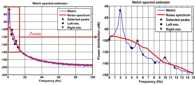
The spectrum using Welch’s method, the detected peaks and the localized minima of each mode of the two signals Sig , and 1 Sig are illustrated in figures 5, and 6 respectively. 2
0 20 40 60 80 100 -220 -200 -180 -160 -140 -120 -100 -80 -60 -40
Welch spectral estimator
Frequency (Hz) P ow e r di s tr ibut ion ( dB ) Welch Noise spectrum Detected peaks Left min. Right min. 0 1 2 3 4 5 6 7 8 9 10 11 12 13 14 15 -160 -140 -120 -100 -80 -60 -40
Welch spectral estimator
Frequency (Hz) P ow e r di s tr ibut ion ( dB ) Welch Noise spectrum Detected peaks Left min. Right min.
Figure 5: The spectrum using Welch’s method, the detected peaks at 1.95, 5.07 & 9.96 Hz, and the localized minima of each mode of Sig 1
The results of the proposed method over the two simulated signals Sig , and 1 Sig are summarized in 2
Tables 3, and 4 respectively.
Mode Filter band (Hz) GA
t Y
T () Level Crossing Local Extrema Positive Point Zero-Up Crossing
Period 4 5 6 7 4 5 6 7 4 5 6 7 4 5 6 7 1st [0-3.90] fˆ 2.00 2.00 2.00 1.99 1.99 1.99 1.99 1.99 2.00 2.00 2.00 1.99 2.00 2.00 2.00 1.99 ξˆ 1.68 1.81 1.82 1.85 1.76 1.82 1.83 1.83 1.84 1.84 1.89 1.89 1.63 1.55 1.61 1.68 2nd [4.10-6.05] fˆ 5.01 5.01 5.01 5.01 5.00 5.01 5.01 5.01 5.01 5.01 5.02 5.02 5.00 5.00 5.01 5.00 ξˆ 2.96 3.19 3.14 2.92 2.97 3.28 3.35 3.22 3.14 3.28 3.23 3.03 3.04 3.27 3.26 3.14 3rd [8.20-11.71] fˆ 9.89 9.88 9.89 9.89 9.78 9.93 9.94 9.96 9.92 9.90 9.87 9.86 9.86 9.86 9.89 9.91 ξˆ 4.12 4.13 4.12 3.93 4.45 4.09 4.06 4.19 4.06 4.18 4.37 4.39 4.12 4.34 4.43 4.19
Table 3: The estimated filter band, natural frequency fˆ , and damping ratio ξˆ of Sig using all the four 1
triggering conditions TYGA(t) 0 20 40 60 80 100 -350 -300 -250 -200 -150 -100 -50 0
Welch spectral estimator
Frequency (Hz) P ow e r di s tr ibut ion ( dB ) Welch Noise spectrum Detected peaks Left min. Right min. 0 0.5 1 1.5 2 2.5 3 3.5 4 4.5 5 -250 -200 -150 -100 -50 0
Welch spectral estimator
Frequency (Hz) P ow e r di s tr ibut ion ( dB ) Welch Noise spectrum Detected peaks Left min. Right min.
Figure 6: The spectrum using Welch’s method, the detected peaks at 0.78, 1.95, & 4.00 Hz, and the localized minima of each mode of Sig 2
Zoom
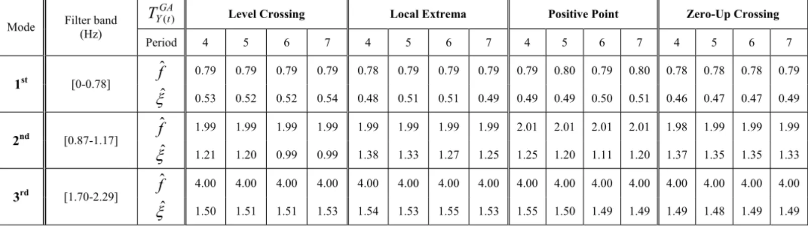
Mode Filter band (Hz)
GA t Y
T () Level Crossing Local Extrema Positive Point Zero-Up Crossing
Period 4 5 6 7 4 5 6 7 4 5 6 7 4 5 6 7 1st [0-0.78] fˆ 0.79 0.79 0.79 0.79 0.78 0.79 0.79 0.79 0.79 0.80 0.79 0.80 0.78 0.78 0.78 0.79 ξˆ 0.53 0.52 0.52 0.54 0.48 0.51 0.51 0.49 0.49 0.49 0.50 0.51 0.46 0.47 0.47 0.49 2nd [0.87-1.17] fˆ 1.99 1.99 1.99 1.99 1.99 1.99 1.99 1.99 2.01 2.01 2.01 2.01 1.98 1.99 1.99 1.99 ξˆ 1.21 1.20 0.99 0.99 1.38 1.33 1.27 1.25 1.25 1.20 1.11 1.20 1.37 1.35 1.35 1.33 3rd [1.70-2.29] fˆ 4.00 4.00 4.00 4.00 4.00 4.00 4.00 4.00 4.00 4.00 4.00 4.00 4.00 4.00 4.00 4.00 ξˆ 1.50 1.51 1.51 1.53 1.54 1.53 1.55 1.53 1.55 1.50 1.49 1.49 1.49 1.48 1.49 1.49
Table 4: The estimated filter band, natural frequency fˆ , and damping ratio ξˆ of Sig using all the four 2
triggering conditions TYGA(t)
For the two simulated signals Sig and 1 Sig we assume the number of modes to be three, and the 2
estimation yields three modes with a very close position to the simulated frequencies. This assures the capability of the estimated noise spectrum to track the modes of interest as shown in Figures 5, and 6.
The high frequency range modes can be easily estimated with the proposed algorithm, i.e. the quality of the estimation is insensitive to the parameter sets. However, the modes with lowest frequency ranges are less precisely estimated because it is easier to be disturbed by the noise and it only can be detected with high false-alarm probability. For modes with narrower frequency band, this effect might be trivial.
From Tables 3, and 4, the performance of the algorithm is relatively robust. Under all the parameter settings, like the different types of triggering conditions and the different number of periods, fixed between 4 and 7 due to the fact that the variance of the RDS increases with the number of cycles [1], the modal parameters were extracted correctly, with values very close to the estimated ones.
6.2 Application on real-world ambient vibration signals
The signal of this part is a real-world ambient vibration signal, recorded at the top of the 27th floor Taipo Tower, the republic of china (Taiwan), Figure 1, using multiple sensors placed on several stories to measure simultaneously the vibrations in three directions, longitudinal, transverse and vertical. This signal is sampled at 200 Hz.
For this signals we study the analysis uniquely over the data in the longitudinal direction. Focusing on the first three modes represented as, the first longitudinal, the first transverse, and the first torsion mode respectively.
The spectrum using Welch’s method, the detected peaks and the localized minima of each mode of Taipo signal are illustrated in Figure 8. The estimation of the modal parameters by the proposed algorithm is shown in Table 5. 0 20 40 60 80 100 100 150 200 250 300 350
Welch spectral estimator
Frequency (Hz) P ow e r di s tr ibut ion ( dB ) Welch Noise spectrum Detected peaks
0
0.5
1
1.5
2
2.5
150
200
250
300
350
Welch spectral estimator
Frequency (Hz)
P ow e r di s tr ibut ion ( dB ) Welch Noise spectrum Detected peaks Left min. Right min.Figure 8: The spectrum using Welch’s method, the detected peaks at 0.40, 1.13, & 2.02 Hz, and the localized minima of each mode of the Taipo signal
Mode Filter band (Hz) GA
t Y
T () Level Crossing Local Extrema Positive Point Zero-Up Crossing
Period 4 5 6 7 4 5 6 7 4 5 6 7 4 5 6 7 1st [0.09-0.71] fˆ 0.40 0.38 0.38 0.39 0.38 0.38 0.39 0.39 0.40 0.39 0.39 0.40 0.39 0.38 0.38 0.39 ξˆ 0.96 0.88 0.93 0.95 1.05 0.98 0.94 0.85 0.99 1.06 1.12 0.98 0.98 0.98 1.05 1.06 2nd [0.72-1.55] fˆ 1.14 1.14 1.13 1.14 1.13 1.13 1.13 1.14 1.13 1.14 1.14 1.14 1.14 1.14 1.13 1.14 ξˆ 1.13 0.92 1.08 0.99 1.19 0.98 0.86 0.85 0.92 1.08 1.10 1.07 1.11 1.10 1.07 1.22 3rd [1.61-2.42] fˆ 2.04 2.03 2.04 2.04 2.04 2.04 2.04 2.04 2.04 2.04 2.04 2.04 2.04 2.04 2.04 2.05 ξˆ 2.02 1.98 1.84 1.88 1.88 2.14 1.93 1.86 2.02 1.96 1.98 2.05 2.50 2.33 2.13 2.07
Table 5: The estimated filter band, natural frequency fˆ , and damping ratio ξˆ of the CHB signal using all the
four triggering conditions TYGA(t)
In the real-world ambient vibration signals, the frequency bandwidth of the modes under study is often very narrow. Figure 8 shows the result of the proposed method on identifying the three modes of interest, based on the a priori physical information about their positions. Despite the frequency closeness of peaks, the noise spectrum estimation and the peak detection methods proposed here are able to detect correctly the three modes.
To further show the applicability of the proposed method, Table 5 summarizes the result of modal parameters estimations. For all the three modes, regardless of the type of triggering condition and the number of period, the fundamental frequencies were extracted correctly as compared to the values of the a priori
Figure 7: The Taipo tower at the city center of Taipei (left), and its geographical location (right)
information from the physicians. On the other hand, the damping ratios were very close in value to each other, which indicate a good functionality of the RDT over this signal.
7 Conclusions
In this paper, we propose an automatic method for setting the RDT processing parameters. The proposed method guides up the automatic choice of the parameters for the filtering process, which is the first step to condition the applicability of the RDT over multicomponent signals.
For the filtering process an automatic bandwidth measurements are achieved by first apply the Welch’s method to have a spectral representation of the signal. At each local spectrum a peak detection method is applied to extract peaks from the noise spectrum, which is first estimated by a multipass filtering. For each detected peak, the corresponding minima are localized with a symmetric test. The test consists of accepting the symmetry of either the left minimum of the right one of the detected peak with a condition that no other mode is included in the symmetry range.
The automatic filtering of each mode is then followed by segmenting the filter output in order then to average the segments and to retrieve an approximate system response with a good modal parameter estimation.
The performance analysis on both the simulated and real-world data show that the proposed method works correctly despite the different types of the triggering conditions and the number of periods that is set with a low range in order not to increase the variance of the estimated RDS. The modal parameters are then estimated with a relative robustness and the modes detected correctly and automatically. This proves that when the filtering process is carried out very carefully, the RDT performance is enhanced and thus the modal parameter estimations.
The proposed method is carried out by adding original techniques in many steps of the RDT with much better adaptability reserving all the important characteristics of the RDT, like the simplicity and the speed, thus allows working on the multi modes of the signal simultaneously with few manual configurations.
Possible extension of the present work includes generalizing the current selection method to the cases when the excitations are seismic.
Acknowledgments
This work has been supported by French Research National Agency (ANR) through RISKNAT program (project URBASIS ANR-09-RISK-009).
References
[1] H. A. Cole, On-the-line Analysis of Random Vibrations, AIAA: ASME Structures, Structural Dynamics and Materials Conference, Palm Springs (1968).
[2] J. K. Vandiver, A. B Dunwoody, R. B Campbell, and M. F. Cook, A Mathematical Basis of the Random
Decrement Vibration Signature Analysis Technique, J. of Mechanical Design, Vol. 104, pp. 307-313,
(1982).
[3] J. Asmuussen, Modal Analysis Based on the Random Decrement Technique: Application to Civil
Engineering Structures, PhD Dissertation, U. of Aalborg, D. (1997).
[4] S. R. Ibrahim, Random Decrement Technique for Modal Identification of Structures, Journal of Spaccecraft and Rockets, vol. 14, No. 11, pp. 696-700 (1997).
[5] J. Antoni and M. El Badaoui, The Discrete-Time Random Decrement Technique: Closed-form Solutions
for the Blind Identification of SIMO Systems, International Conference on SSI (2011).
[6] A. Zubaydi, The Filtering Effect of Random Responses of Stiffened Plates on Their Random Decrement
Signatures and Natural Frequencies, Majalah IPTEK, Vol. 16, No. 1, (2005).
[7] J.C.S Yang, N. Dagalakis, and M. Hirt, Application of the Random Decrement Technique in the
Detection of an Induces Crack on an Offshore Platform Model, Computer Methods for Offshore Structures. ASME, 165-21, pp. 55-67, (1980).
[8] M. Durnerin, “A strategy for interpretation in spectral analysis,” Ph.D. dissertation, Institut National Polytechnique de Grenoble, France, 1992.
[9] C. Mailhes, N. Martin, K. Sahli, and G. Lejeune, “A Spectral Identiy Card,” in EUropean SIgnal Processing Conference, EUSIPCO 06,, Florence, Italy, 2006.
[10] N. Martin, Spectral Analysis, Parametric, Non-parametric and Advanced Methods, F. CASTANIE, Ed. WILEY-VCH, 2011.
[11] F. Millioz and N. Martin, “Time-Frequency Segmentation for Engine Speed Monitoring,” in ICSV13, Vienna, Austria, July 2-6 2006.
[12] S. M. Kay and R. Sudhaker, "A Zero Crossing Based Spectrum Analyzer," IEEE Trans. Acoust., Speech, Signal Processing, Vol. ASSP-34, pp. 96-104, February 1986.
[13] C. Michel, S. Hans, P. Gueguen, and C. Boutin, “In Situ Experiment and Modelling of RC-Structure Using Ambient Vibration and Timoshenko Beam”, First European Conference on Earthquake Engineering and Seismology, Switzerland 2006.
![Figure 1: Flow chart of the global algorithm. Given the input signal y [ ] t , the algorithm provides the number of peaks Q , the bandwidth and the segment length estimations, using the parameters L f , PFA γ ,](https://thumb-eu.123doks.com/thumbv2/123doknet/14545192.536081/5.892.137.764.414.650/figure-algorithm-algorithm-provides-bandwidth-segment-estimations-parameters.webp)