HAL Id: hal-01966044
https://hal.archives-ouvertes.fr/hal-01966044
Submitted on 27 Dec 2018
HAL is a multi-disciplinary open access
archive for the deposit and dissemination of
sci-entific research documents, whether they are
pub-lished or not. The documents may come from
teaching and research institutions in France or
abroad, or from public or private research centers.
L’archive ouverte pluridisciplinaire HAL, est
destinée au dépôt et à la diffusion de documents
scientifiques de niveau recherche, publiés ou non,
émanant des établissements d’enseignement et de
recherche français ou étrangers, des laboratoires
publics ou privés.
Distributed learning with kernels in wireless sensor
networks for physical phenomena modeling and tracking
Cédric Richard, Paul Honeine, Hichem Snoussi, André Ferrari, Céline Theys
To cite this version:
Cédric Richard, Paul Honeine, Hichem Snoussi, André Ferrari, Céline Theys. Distributed learning
with kernels in wireless sensor networks for physical phenomena modeling and tracking. Proc. IEEE
International Geoscience and Remote Sensing Symposium (IGARSS), 2010, Honolulu (Hawaii), USA,
United States. �hal-01966044�
DISTRIBUTED LEARNING WITH KERNELS IN WIRELESS SENSOR NETWORKS
FOR PHYSICAL PHENOMENA MODELING AND TRACKING
Cédric Richard
(1), Paul Honeine
(2), Hichem Snoussi
(2), André Ferrari
(1), Céline Theys
(1)(1)Laboratoire Fizeau (UMR CNRS 6525, OCA), Université de Nice Sophia-Antipolis, 06108 Nice, France
(1)Institut Charles Delaunay (FRE CNRS 2848), Université de technologie de Troyes,10010 Troyes, France
Wireless ad-hoc sensor networks have emerged as an interesting and important research area in the last few years. They rely on sensor devices deployed in an environment to support sensing and monitoring, including temperature, humidity, motion, acoustic, etc. Low cost and miniaturization of sensors involve limited computational resources, power and communication capacities. Consequently, wireless ad-hoc sensor networks require collaborative execution of a distributed task on a large set of sensors, with reduced communication and computation burden.
In this paper, we consider the problem of modeling physical phenomena such as temperature field distributions, and track their evolution. Many approaches have been proposed in the signal processing literature to address this issue with collaborative sensor networks. In the framework of distributed inference with parametric models, focus was clearly put on determining how the channel capacity limits the quality of estimates. See, e.g., [1] and references inside. Model-based techniques were also exploited to compress the data based on their temporal and spatial redundancy [2]. Since they do not depend on some arbitrary modeling assumptions, applications of wireless sensor networks provide a strong motivation for the use of nonparametric methods for decentralized inference. See [3] for a survey. Model-independent methods based on kernel machines have recently been investigated. In particular, a distributed learning strategy has been successfully applied to regression in wireless sensor networks [5]. In this paper, we take advantage of this framework to derive a new approach.
Kernel-based methods have gained wide popularity over the last decade. Initially derived for regression and classification with support vector machines, they include classical techniques such as least-squares methods and extend them to nonlinear functional approximation. We wish to determine a function ψo(·) defined on the area of interest X that best models a distribution
such as a temperature field. The latter is learned from the information coupling sensor locations and measurements. The information from the N sensors located at xn ∈ X which provide measurements dn ∈ lR, with i = n, . . . , N , is combined in the set of pairs{(x1, d1), . . . , (xN, dN)}. Consider a reproducing kernel κ : X × X → lR. Let us denote by H its reproducing kernel Hilbert space (RKHS) with inner producth· , ·iH. This means that every function ψ ofH can be evaluated at any x∈ X by ψ(x) = hψ, κxiH, where κxdenotes κ(·, x). This allows us to write κ(xi, xj) = hκxi, κxjiH, which defines the reproducing property. One of the most widely used kernel is the Gaussian kernel κ(xi, xj) = e−kxi−xjk
2/2σ2
kernel bandwidth. We seek the optimal ψothat minimizes the following global cost function J(ψ) = N X n=1 E|ψ(xn) − dn|2,
that is, J(ψ) =PNn=1E|hψ, κxniH− dn|2using the reproducing property. The cost function J(ψ) can be rewritten as follows, for any node k∈ {1, . . . , N },
J(ψ) = Jk(ψ) + N X n=1 n6=k Jn(ψ)
with Jk(ψ) =Pn∈Nkcn,kE|hψ, κxniH− dn|2the local cost function, andNk the set of neighbors of sensor k. Here, cn,k is the(n, k)-th component of C, which satisfies the following constraints: cn,k= 0 if n 6∈ Nk, C11 = 11 and 11⊤C= 11⊤. Let us write ψon= arg minψ∈HJn(ψ). Finally, it is equivalent to minimize J(ψ) or the following cost function
Jkℓ(ψ) = X n∈Nk cn,kE|hψ, κxniH− dn|2+ N X n=1 n6=k kψ − ψo nk2Hn
Minimizing Jkℓ(ψ) requires the nodes to have access to global information ψo
n. To facilitate distributed implementations, consider the relaxed local cost function
Jkr(ψ) = X n∈Nk cn,kE|hψ, κxniH− dn|2+ X n∈Nk/{k} bn,kkψ − ψnok2H
where ψno is now the best estimate available at node n. The iterative steepest-descent approach for minimizing Jkr(ψ) can be
expressed in the following form
ψk,i= ψk,i−1− µ 2∇J r k(ψk,i−1) with ∇Jr k(ψk,i−1) = X n∈Nk 2 cn,kE(ψk,i−1(xn) − dn) κxn+ X n∈Nk/{k} 2 bn,k(ψk,i−1− ψon)
Incremental algorithms are useful for minimizing sums of convex functions. They consist of iterating sequentially over each sub-gradient, in some predefined order. This leads to the following possible distributed learning strategies.
1. Adapt-then-Combine kernel LMS
For each time instant i and each node k, repeat
φk,i= ψk,i−1− µkPn∈Nkcn,k(ψk,i−1(xn) − dn,i) κxn
ψk,i=Pn∈Nkbn,kφk,i
2. Combine-then-Adapt kernel LMS
For each time instant i and each node k, repeat
φk,i−1=Pn∈Nkbn,kψk,i−1
0.01 0.01 0.01 0.08 0.08 0.08 0.15 0.15 0 .15 0.23 0.23 0.2 3 0 .3 0.3 0.37 0.37 0.44 0.03 0.03 0.03 0.03 0 .2 2 0.22 0.22 0 .22 0.22 0.41 0.41 0.41 0 .4 1 0 .41 0.6 0.6 0.6 0.8 0.8 0 .8 0.98 0.98 1.17 0.12 0.12 0.12 0.12 0.12 0.12 0 .43 0.43 0.43 0.43 0.43 0.43 0 .43 0 .7 0.7 0.7 0.7 0.7 1 1 1 1 1 .3 5 1.35 1.35 1.35 1.6 6 1.66 1.66 1.97 1.97
Fig. 1.Snapshots of the evolution of the estimated temperature at t = 100 (left), t = 150 (center) and t = 200 (right). Sensors are shown
with small blue dots. Big red dots represent the sensors of interest according to a criterion that will be described in the camera-ready paper.
Both strategies consist of adapting local regressors based on measurements, and combining them if they are in the neighborhood of each other. Measurements and regressors are not exchanged between the nodes if cn,k = δn,k. In what follows, each cn,k and bn,k were set to|Nk|. To illustrate the relevance of our technique, we considered a classical application of estimating a temperature field governed by the partial differential equation
∂Θ(x, t)
∂t − c∇
2
xΘ(x, t) = Q(x, t).
HereΘ(x, t) denotes the temperature as a function of space and time, c is a medium-specific parameter, ∇2
xis the Laplace spatial operator, and Q(x, t) is the heat added. We studied the question of monitoring the evolution of the temperature field
distribution in a square region with open boundaries and conductivity c= 0.1, using N = 100 sensors deployed randomly on
a grid. Given some measurements dn,i = Θ(xn, ti) + zn,i, with zn,ia i.i.d. Gaussian noise, the problem was to estimate the temperatureΘ(xn, ti) via ψi(xn) based on the Gaussian kernel.
Two heat sources of intensity200 W were placed within the region, the first one was activated from t = 1 to t = 100,
and the second one from t = 100 to t = 200. The experimental setup will be described in the camera-ready paper. Fig. 1
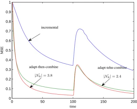
illustrates the estimated temperature field distribution at different times by the Adapt-then-Combine strategy, for several values of|Nk|. The convergence of the proposed algorithm is illustrated in Fig. 2 where we show the evolution over time of the normalized mean-square prediction error. The abrupt change in heat sources at t= 100 is clearly visible, and highlights the
convergence behavior of the proposed algorithm. Comparison with an iterative distributed gradient algorithm clearly shows a faster convergence speed.
0 50 100 150 200 0 0.1 0.2 0.3 0.4 0.5 0.6 0.7 0.8 0.9 1 time M S E incremental adapt-then-combine adapt-tehn-combine |Nk| = 3.8 |Nk| = 2 .4
Fig. 2.Learning curve obtained from t = 1 to t = 200. Time t = 100 corresponds to a system modification.
1. REFERENCES
[1] A. Swami, Q. Zhao, and Y.-W. Hong, Wireless Sensor Networks: Signal Processing and Communications. Wiley, 2007.
[2] C. Guestrin, P. Bodi, R. Thibau, M. Paski, and S. Madde, “Distributed regression: an efficient framework for modeling sensor network data,” in Proc. third international symposium on information processing in sensor networks (IPSN). New York, NY, USA: ACM, 2004, pp. 1–10.
[3] J. B. Predd, S. R. Kulkarni, and H. V. Poor, “Distributed learning in wireless sensor networks,” IEEE Signal Processing Magazine, vol. 23, no. 4, pp. 56–69, 2006.
[4] ——, “Distributed regression in sensor networks: Training distributively with alternating projections,” CoRR, vol. abs/cs/0507039, 2005, informal publication.