HAL Id: hal-01915349
https://hal.uca.fr/hal-01915349
Submitted on 21 Oct 2019
HAL is a multi-disciplinary open access
archive for the deposit and dissemination of
sci-entific research documents, whether they are
pub-lished or not. The documents may come from
teaching and research institutions in France or
abroad, or from public or private research centers.
L’archive ouverte pluridisciplinaire HAL, est
destinée au dépôt et à la diffusion de documents
scientifiques de niveau recherche, publiés ou non,
émanant des établissements d’enseignement et de
recherche français ou étrangers, des laboratoires
publics ou privés.
Improving thin structures in surface reconstruction from
sparse point cloud
Maxime Lhuillier
To cite this version:
Maxime Lhuillier. Improving thin structures in surface reconstruction from sparse point cloud. ECCV
2018 workshops, 11129, Springer, pp.443-458, 2019, Lecture notes in computer science,
�10.1007/978-3-030-11009-3_27�. �hal-01915349�
reconstruction from sparse point cloud
Maxime Lhuillier1[0000−0002−7405−8171]
Universit´e Clermont Auvergne, CNRS, SIGMA Clermont, Institut Pascal, F-63000 Clermont-Ferrand, France
[email protected] maxime.lhuillier.free.fr
Abstract. Methods were proposed to estimate a surface from a sparse cloud of points reconstructed from images. These methods are interesting in several contexts including large scale scenes, limited computational resources and initialization of dense stereo. However they are deficient in presence of thin structures such as posts, which are often present in both urban and natural scenes: these scene components can be partly or even completely removed. Here we reduce this problem by introducing a pre-processing, assuming that (1) some of the points form polygonal chains approximating curves and occluding contours of the scene and (2) the direction of the thin structures is roughly known (e.g. vertical). In the experiments, our pre-processing improves the results of two different surface reconstruction methods applied on videos taken by helmet-held 360 cameras.
Keywords: Thin structures · Sparse features · 3D Delaunay triangula-tion · Visibility · Environment modeling
1
Introduction
The automatic surface reconstruction from images is still an active research topic. One of the difficulties is caused by thin structures: they are partly or even com-pletely removed by the methods that do not include specific processing. There are two kinds of thin structures: planar ones like road signs and rectilinear ones like posts. This paper only focuses on the rectilinear case, which is frequent in both urban and natural scenes. It also focuses on an input point cloud recon-structed from sparse features in images. This is useful not only for applications that do not need the high level of details of computationally expensive dense stereo, but also to initialize dense stereo in other cases. Since we have two diffi-culties (thin structures and sparse input) and would like a tractable problem, our method uses further information available in the images: we reconstruct curves as polygonal chains in 3D from image gradient. We also assume that the thin structures have a known direction with large tolerance. The paper restricts to the vertical direction which is the dominant direction of the reconstructed curves in our terrestrial image sequences (this is partly due to the aperture problem), but it is obvious to consider several directions by alternating.
2
Previous surface reconstruction methods
We summarize methods that use constraints similar to ours, whether they deal with thin structures or not, without or with a sparse point cloud.
2.1 Using lines or curves or image gradient
Methods use lines or curves and organize them as graphs, which are used as scaffolds for surface reconstruction. In [22], curves are reconstructed from image gradient and the surface is obtained by curve interpolation (lofting) and occlusion reasoning. In [24], an initial surface mesh is regularized by back-projecting linear structures that are semi-automatically selected from the images. Other methods estimate dense depth maps including pixels at occluding contours, then merge them in a voxel grid. In [18], quasi-dense depth maps of internet images are densified by encouraging depth discontinuities at image contours. In [27], the depths of video sequences are first computed in high-gradient regions including silhouettes, then they are propagated to low-gradient regions. Using a point cloud reconstructed from images of a scene with planar structures, [5] segments into inside and outside a tetrahedralization of the points by using graph-cut and two regularizations: horizontal slicing and a smoothness term based on image lines.
A very recent work [10] deals with thin rectilinear structures. First it recon-structs curves from image gradient, then integrates both dense scattered points and curve vertices in a 3D Delaunay triangulation, last segments into inside and outside by using graph-cut.
2.2 Reconstructing trees and roots
Methods estimate thin structures like trees [20, 12] and plant roots [28]. In [12], several trees are automatically reconstructed from laser scan data assuming that the major branch structures are sampled. First every tree is modeled by a min-imal spanning tree whose root is on high point density of the ground plane, vertices are input points and edge weights are Euclidean distances. Then the spanning trees are globally optimized using constraints on length, thickness and smoothness derived from biological properties. A previous method [20] recon-structs realistic-looking trees from pre-segmented images into branches/leaves/ background and a more difficult point cloud estimated by quasi-dense structure-from-motion. The computation of minimum spanning trees is done for subsets of branches using weights combining two distances (3D Euclidean and image gradient-based). Little user interaction is needed to select branch subsets and to connect subsets. The method in [28] is shortly summarized in two steps: first robustly estimate a visual hull of the plant roots (They are mostly black with white background thanks to a transparent gel container.) in a voxel grid, then re-pair the connectivity of the inside voxels by computing a minimal spanning tree. In these methods and [10], the connectedness constraint is essential to recover missing parts of the thin structures.
2.3 Other surface reconstruction methods
Other methods are not in the classifications above. In [1], the input point cloud is first approximated by planar segments, then these segments are prolonged and assembled into a well-behaved surface using visibility constraints. The prolonga-tions are done using prior on urban scenes including the prevalence of the vertical structures. In [6], a graph-cut method segments a tetrahedralization of the input points into inside and outside by using visibility information. Compared to [23], it favors the inside where the visibility gradient is high and improves the thin structure reconstructions, but it ignores image gradient and tends to produce more surfaces that do not correspond to real surfaces. In [16], thin structures such as stick and rope are reconstructed in a voxel grid by enforcing the inside connectedness. First an approximate visual hull including the final surface is estimated, then a voxel labeling is computed by convex optimization subject to linear constraints on the labeling derivatives such that the inside and the visual hull have similar topology. Thin planar structures [21] are not the paper topic.
2.4 Our contribution
There are several differences between our method and the previous ones that reconstruct thin (rectilinear) structures. First we reconstruct 3D curves from image gradient (including those that approximate occluding contours) and use them to detect the thin vertical structures. Their points also complete the sparse input point cloud reconstructed by structure-from-motion (SfM). Second we par-tition the space by using a 3D Delaunay triangulation T of the input points with tetrahedra labeled freespace or matter. Voxel grid is used in most previous works for thin structures but is inadequate for both large scale scenes and sparse in-put point cloud. Third we detect the thin structures in T as vertices of vertical curves that have small matter neighborhoods in the horizontal directions. These vertices are regrouped in large enough sets to avoid false positive detections. There is only one thin structure per set. Fourth we use the connectedness con-straint to complete the thin structures in the vertical direction: force to matter vertical series of tetrahedra connecting vertices of a same set. Last we adapt two previous surface reconstruction methods such that their regularizations do not cancel our matter completion.
Now we detail differences with the closest and recent work [10]. It adds to T a lot of Steiner vertices near 3D curves, which are not in the original input and do not have visibility information (i.e. rays). This is not adequate for incremental surface reconstruction methods like [11, 17] and is not obvious to adapt to non-graph-cut methods. Our thin structure processing does not use such points and does not have these drawbacks. The price to pay is (1) an approximate knowl-edge of the direction of thin structures and (2) involved detection-completion steps of the matter tetrahedra of the thin structures. Furthermore we start with terrestrial video sequences with sparse point clouds. We believe that this exper-imental context is more challenging (or “wild”) than that of [10], which starts from denser point clouds and still images whose view-points are selected by UAV.
3
Overview
The three first steps in Secs. 3.1, 3.2 and 3.3 estimate the curves, the vertical direction and initialize the 3D Delaunay triangulation from the output of a sparse SfM. The two next steps in Secs. 3.4 and 3.5 are the main contributions: they detect the thin vertical structures and improve their matter labeling. Last Secs. 3.6 and 3.7 explain how to update two surface reconstruction methods to take into account our matter improvement: a graph-cut method in [23] and a manifold method in [9].
3.1 Step 1: estimate points and polygonal chains
We use standard methods: detect both Harris points and Canny curves, match them in consecutive images of the sequence using correlation and the epipolar constraint [8]. A curve is approximated by a polygonal chain of points in an image such that the distance between two consecutive points is roughly constant (4 pixels in our implementation). These points are matched with points of Canny curves in other images. Then the chain points are reconstructed independently and we obtain a polygonal chain in 3D. Last all 3D points are filtered by thresh-olding on angles formed by their rays. (Reject a point if its angles are smaller than 10 degrees.) Better methods exist to reconstruct lines and curves [7, 13, 4, 2], but this is not the paper focus. The resulting polygonal chains approximate curves in 3D and have both redundancy and inaccuracy for several reasons: fail-ures of detection and matching, matching of 2D points that do not correspond to a single 3D point due to occluding contours, inaccurate camera calibration.
3.2 Step 2: estimate the vertical direction
In the terrestrial imaging context, we observe that the main direction of the edges of the polygonal chains is vertical. (There are also a lot of horizontal curves in usual scenes, but most of them cannot be reconstructed due to the aperture problem.) Thus we compute the density of the edge directions in a histogram and assume that the direction with the largest density is vertical.
3.3 Step 3: initialize the 3D Delaunay triangulation
Step 3 is a by-product of the surface reconstruction methods based on 3D Delau-nay triangulation and visibility constraints. First a 3D DelauDelau-nay triangulation T is build from the points generated in Sec. 3.1. Then its tetrahedra are labeled freespace or matter. In more details, each Delaunay vertex a has several rays and a ray is a line segment ac between a and a viewpoint c whose image includes a detection of a. The matter M is the set of tetrahedra that are not intersected by ray(s) and T \ M is the freespace. Note that we not only have isolated points but also edges of polygonal chains. Following [3, 19], a tetrahedron is freespace if it is intersected by a stereo triangle abc where ab is such an edge and c is a common viewpoint of a and b (more details in the supplementary material).
3.4 Step 4: detect vertices of the thin structures
For each thin structure, we would like to find (as large as possible) sets of vertices of T that are in the structure. Such a set is computed as a connected component of a graph G with vertex set V and edge set E. Since structure is vertical, all edges in E are almost vertical. The set E not only includes edges of the polygonal chains but also edges of the Delaunay triangulation. (A same structure can have many polygonal chains.) Since structure is matter, every vertex in V is in at least one matter tetrahedron in M . Since structure is thin along the vertical direction, such a vertex has a small connected component of matter tetrahedra in a horizontal neighborhood (in a slice between two horizontal planes). Sec. 4.2 details the definition of G.
Evidence of thin structure increases with connected component size. Thus we reject the smallest connected components of G to avoid false positive detections of thin structures. (If they have less than 6 vertices in our implementation.)
3.5 Step 5: improve the matter of the thin structures
Thin vertical structure should be approximated in T by connected set of matter tetrahedra with large size in the vertical direction and small size in the horizontal directions. However, this connectedness does not hold in practice due to several reasons: noise, lack of points and bad points that generate false positive freespace tetrahedra. We would like to improve this connectedness by using the selected connected components of G (Sec. 3.4).
Since all vertices of a connected component C of G are in a same structure, we force to matter (i.e. add to M ) series of tetrahedra in T connecting vertices of C. Since structure is vertical, the forced tetrahedra cover line segments that are almost vertical. Since structure is thin, we only force to matter tetrahedra with small size in the horizontal directions. Thus there are two steps: first estimate the width (measuring the size in the horizontal directions) of the structure including C, then complete M by considering tetrahedra between pairs of vertices in C if the width of these tetrahedra are not too large compared to that of the structure. This process is detailed in Sec. 4.3.
Last we set a Boolean b∆for every tetrahedron ∆: b∆is true if and only if ∆
is forced to matter by Step 5. (Whether we have ∆ ∈ M or ∆ /∈ M in Step 3.)
3.6 Step 6a: graph-cut surface reconstruction
The graph-cut method [23] labels the tetrahedra of T with inside or outside. (The surface is the triangle set between outside and inside tetrahedra.) How-ever, it removes thin structures by labeling outside several tetrahedra that are in M . There are two reasons: it has a regularization and it ignores our mat-ter improvement. Thus we modify it such that the set of the inside tetrahedra includes the set of the tetrahedra with true Boolean b∆ (Sec. 3.5).
We remind that it computes a minimum s − t cut of a graph. This graph is the adjacency graph of T augmented by two vertices {s, t} and edges {vs, vt}
for every vertex v of the adjacency graph. Cut is partition of the vertex set in two subsets: a subset including s and a subset including t. The details on the definition of the augmented graph and its edge weights are in [23]. We only need to know that if vt has a large weight, v and t are in the same subset, which implies that the tetrahedron associated to v is labeled inside.
Thus we modify the augmented graph (before computing the minimum cut) by adding a large value to every edge vt such that the tetrahedron ∆ associated to v has a true Boolean b∆.
3.7 Step 6b: manifold surface reconstruction
The manifold method [9] also labels the tetrahedra of T with inside or outside. It uses our matter improvement (i.e. the set M computed in Sec. 3.5), but it removes thin structures due to a regularization, which labels outside several tetrahedra that are in M .
We summarize it to correct the regularization. Let O be the set of outside tetrahedra and ∂O be its boundary, i.e. the set of triangles between outside and inside tetrahedra. First O grows in T \ M to meet visibility constraints, then O evolves in T by the regularization. Both steps maintain the manifoldness of ∂O. The regularization removes peaks, i.e. rings of triangles in ∂O around a vertex a which form small solid angles. This is done in two cases: remove from O all tetrahedra including a, or add to O all tetrahedra including a. However parts of thin vertical structure can be removed in the second case: some of their matter tetrahedra can become outside the surface.
We solve this problem as follows: the regularization is prohibited in the second case if at least one of the tetrahedra added to O has a true Boolean b∆.
4
Detection and improvement of the structures
Here we detail the contributions of the paper summarized in Secs. 3.4 and 3.5.
4.1 Definitions
We remind that M is the set of the matter tetrahedra in T , which should include the thin vertical structures. Let v ∈ R3 be the vertical direction. (We have ||v|| = 1.)
The small matter slice M (∆0) started from a tetrahedron ∆0 ∈ M is
com-puted as follows. Let P1 and P2 be the two horizontal planes that enclose ∆0.
(The vertex of ∆0with the highest or lowest altitude is in P1or P2, both altitude
and horizontal directions are defined using v.) We initialize M (∆0) = {∆0} and
complete it by a graph traversal of the adjacency graph of M by only consider-ing tetrahedra that intersect the area between P1 and P2. In more details, the
following process is repeated: take a tetrahedron ∆ ∈ M (∆0) and add to M (∆0)
every neighbor tetrahedron of ∆ in M (∆ has no more than four neighbors) that intersects the area between P1and P2. We only need matter slices whose number
of tetrahedra is less than a small threshold Mmax, i.e. which can be included in
a thin vertical structure. (We use Mmax= 20.) Thus we stop the graph traversal
if M (∆0) becomes larger than Mmax, then we reset M (∆0) = ∅ (no slice found).
Let a and b be in R3. The horizontal distance w(a, b) is
w(a, b) = q
||a − b||2− (v>(a − b))2. (1)
Let v(A) be the vertex set of a tetrahedron set A ⊆ T . The maximum width of A is measured from a base point b ∈ R3:
w(A, b) = max{w(a, b), a ∈ v(A)}. (2) We also define the path p(∆, a) between a tetrahedron ∆ ∈ T and a vertex a ∈ v(T ): this is the set of tetrahedra in T whose interiors are intersected by the line segment joining a and the barycenter of ∆.
4.2 Vertex detection
We only need to detail the definition of the graph G = (V, E) introduced in Sec. 3.4. Let α be an angle threshold. Let E0 be the set of the edges ab in the polygonal chains that are almost vertical, i.e. if
|v> b − a
||b − a||| > cos α. (3) We use a large tolerance α = 20◦is our implementation. Let V0be the vertex set of E0. We have a ∈ V if and only if a ∈ V0 and there is a tetrahedron ∆0∈ M
including a such that M (∆0) 6= ∅. We have ab ∈ E if and only if a ∈ V and
b ∈ V and Eq. 3 is meet and the following condition is meet: ab ∈ E0 or ab is an edge of the Delaunay triangulation or there is c ∈ V0 such that ac ∈ E0 and cb ∈ E0. The last condition using c ∈ V0 is useful to connect two parts of a thin structure separated by a vertex that is not in a matter tetrahedron.
4.3 Matter improvement
First we estimate a median width wCfor every connected component C of G by
using the horizontal distance between a vertex b ∈ C and other vertices of the small matter slices M (∆0) such that b ∈ ∆0. We collect the small matter slices
attached to b ∈ C in
Mb= ∪b∈∆0∈MM (∆0) (4)
and compute
wC= median{w(a, b), b ∈ C, a ∈ v(Mb), a 6= b}. (5)
Second the vertices ai ∈ C are ordered along the vertical direction v: they
a2a3, · · · for C, which should be included in matter tetrahedra of the thin
structure (it is not expected to be exactly on the surface of the thin structure). Third we collect in a list L for several pairs (i, j) a path between ai and
aj that will be forced to matter. Let b = (ai + aj)/2. We consider several
paths between ai and aj and take one that minimizes the maximum width with
respect to b. These paths are p(∆, aj) where ai ∈ ∆ ∈ M and p(∆, ai) where
aj∈ ∆ ∈ M . For example, p(∆, aj) minimizes the maximum width for a given
(i, j). If w(p(∆, aj), b) < cwC where c is a threshold, we decide that p(∆, aj)
is thin enough to be forced to matter and we add (∆, aj) to the list L. This is
done for all C. In the experiments, we use c = 2 and only take j ∈ {i + 1, i + 2}. Last the matter is improved: we add p(∆, aj) to M for every (∆, aj) ∈ L.
Fig. 1 summarizes the construction and the use of a composite polygonal chain.
Fig. 1. Construction and use of a composite polygonal chain in a simplified case: in 2D using j = i + 1 without the width test. (The vertical direction is horizontal in this figure.) First there are three reconstructed polygonal chains (bold edges) in the Delaunay triangulation. The gray triangles are matter and the remainder is freespace. Second the vertices of these chains form a connected component of G and we draw the resulting composite polygonal chain (eight bold edges). Third we draw all line segments linking the barycenter of matter triangles and vertices such that j = i + 1. Fourth all triangles intersected by these segments are forced to matter.
5
Experiment
Steps 1-5 (our pre-processing) are described in Sec. 5.1. Secs. 5.2 and 5.3 focus on step 6a (graph-cut methods) and step 6b (manifold methods), respectively. Last Sec. 5.4 shows a lot of results for all surface reconstructions methods. For fair comparisons, the experimented methods start from the same 3D Delaunay tetrahedralization T and end by the same Laplacian smoothing of the surface.
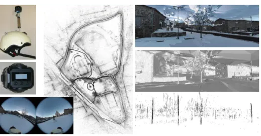
First we take two 2496 × 2496 videos at 30Hz by walking during 473s in a town using a helmet-held 360 camera (Garmin Virb 360). Then we apply generic SfM [14] followed by detection and closure of loops inspired by [26, 25]. Last we experiment on the 1334 keyframes selected by SfM. Fig. 2 shows our setup, a keyframe, a top view of the SfM result, a view of the 3D model by one of our method, and the set of vertical edges that we use.
5.1 Our pre-processing
Step 1 generates 106k polygonal chains having 249k vertices. Step 3 builds the 3D Delaunay triangulation T . It has 1.2M vertices reconstructed from image
Fig. 2. Left: the helmet-held Garmin Virb 360 camera and one keyframe. Middle: a top view of the SfM point cloud and the camera trajectory. Right: A view of the final surface reconstructed by step 6b and the vertical edges (the set E0) that we use.
features and 7.4M tetrahedra, 3.1M of them are matter. Step 4 is the detection step of thin structures. It only retains 25k edges of the polygonal chains that are almost vertical (the set E0). Then it finds 13k vertices in the vertex set of E0 that have a small matter slice in their neighborhood (the set V ). Using edges in both Delaunay triangulation and E0, the graph G has 7k connected components. Last Step 4 only retains 230 of them by ignoring the smallest ones (very end of Sec. 3.4). Step 5 is the matter improvement step. It forces 10k tetrahedra to be matter. (6.5k of them were in T \ M before.) Fig. 3 shows our pre-processing: it has a noticeable improvement on a low-textured thin structure with missing matter tetrahedra and a negligible effect on a well-textured thick structure with a lot of matter tetrahedra. These results are those expected.
The detection and improvement steps take less than 0.6s on a standard lap-top. The feature reconstruction (both Canny and Harris points) is the most time consuming step: 40 minutes.
5.2 Graph-cut surface reconstruction methods
Here we compare methods “base graph-cut” and “our graph-cut”. The former is in [23] and the latter is an update of the former (Sec. 3.6) preceded by our pre-processing (Sec. 3). We remind that base graph-cut estimates a surface min-imizing an energy Evis+ λqualEqual with a visibility term Evis(using αvis= 1)
and a quality term Equal. The greater the value of λqual, the better the
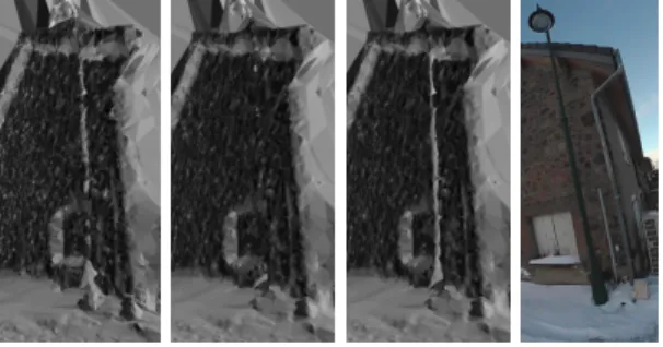
sur-face quality in a regularization sense. Fig. 4 shows a light post reconstructed by our graph-cut using λqual = 2 and base graph-cut using λqual = 0.5 and
Fig. 3. Our pre-processing for a post (top) and a trunk (bottom). From left to right: one input image, reconstructed vertical edges (using α = 20◦), matter tetrahedra before our pre-processing, composite polygonal chains, matter tetrahedra after our pre-processing, final surface.
triangles, respectively. First we see that choosing a small λqualis a first solution
to improve the post. However this solution is not satisfactory for two reasons: the post is incomplete (about 30% is lacking) and the noise increases in the background house. See the gray level variations in the left part. The smaller the value of λqual, the greater the number of surface vertices. (They include
inaccu-rate points.) Second, we see that our graph cut provides the most complete post at the price of very small increases of triangle number and computation time. In the next experiments using base or our graph-cut, λqual = 2.
5.3 Manifold surface reconstruction methods
Now we compare methods “base manifold” and “our manifold”. The former is in [9] and the latter is an update of the former (Sec. 3.7) preceded by our pre-processing (Sec. 3). Fig. 5 shows the same light post as Fig. 4 reconstructed by base manifold and our manifold. The surface of the complete scene has 1.734M and 1.739M triangles, respectively. Almost all parts of the post are removed by base manifold. In contrast to this, the post is almost complete by our manifold (at the price of very small increases of triangle number and computation time). There are two spurious handles that connect the post and the house. Thanks to other examples, we observe that the probability of such an artifact increases when the distance between a post and another scene component (house or wall or another post) decreases.
Fig. 4. Comparing three graph-cut methods. From left to right: base graph-cut using λqual = 0.5, base graph-cut using λqual = 2, our graph-cut using λqual = 2, a local
view of an input image.
Fig. 5 also shows base manifold with the regularization update in Sec. 3.7, and our manifold without the regularization update (i.e. base manifold with our pre-processing). In both cases, the post reconstruction is less complete than that of our manifold. This shows that both our pre-processing and regularization update are useful.
Fig. 5. Comparing four manifold methods. From left to right: base manifold, base man-ifold with updated regularization, our manman-ifold with naive regularization, our manman-ifold, a local view of an input image.
5.4 Other experiments
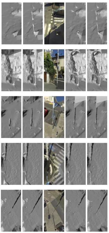
In other examples we compare base graph-cut and our graph-cut, base manifold and our manifold. Fig. 6 shows results for electric posts similar to that in the experiments above with different backgrounds. Our methods provide the most complete post reconstructions. Examining the background house in the top of the figure and assuming its planarity, we compare noises: the graph-cut noise is
greater than the manifold noise although the total numbers of surface triangles are similar. Examining the post in the bottom of the figure, we note a shrinking artifact due to the Laplacian smoothing and a fattening artifact due to low texture in the background. (There is a lack of points to carve the freespace near the post bottom, thus the foreground post and background are not separated.) This holds for all methods. Figs. 7 and 8 show thin structures in another dataset: a 2.5km long sequence using four helmet-held Gopro cameras biking in a city [15]. Although our results on thin structures are not perfect, they are clearly better than those of the two base methods which omit important parts. Furthermore we remind that they are obtained in a difficult context: sparse point clouds from videos sequences taken in the wild.
We also examine the differences between base methods and our methods in overall reconstructed scenes, and see few blunders of our preprocessing due to excesses of the matter completion. There are several reasons. A first one is the conservative selection of vertices in Sec. 3.4: the small connected components of G are discarded for robustness (for both detection and wCcomputation). Second
our matter completion forces only 10k tetrahedra to matter. This number is small compared to the 3.1M tetrahedra that are matter by default, i.e. that are not intersected by rays or stereo triangles in Sec. 3.3. Third the tetrahedra forced to matter are selected in Sec. 4.3 such that they have smallest widths as possible in the horizontal directions. This limits the size of a potential blunder.
Fig. 6. Comparisons between several methods. From left to right: base graph-cut, our graph-cut, local view of input image, base manifold, our manifold.
Fig. 7. Comparisons between several methods. From left to right: base graph-cut, our graph-cut, our manifold (textured), base manifold, our manifold.
Fig. 8. Comparisons between several methods. Top: base graph-cut (left) and our graph-cut (right). Middle: base manifold (left) and our manifold (right). Bottom: local view of an input image.
6
Conclusion
This paper presents a new pre-processing to improve the thin rectilinear struc-tures in a surface reconstructed from an image sequence using a sparse cloud of features and their visibility. Starting from the traditional 3D Delaunay tri-angulation, we first detect vertical series of vertices in a same thin structure by reconstructing curves. Then we complete the matter label in tetrahedra between such vertices by using the connectedness constraint. Last we easily adapt two previous surface reconstruction methods such that their regularizations do not remove the thin structures that we detect and complete.
Our method has limitations and can be improved by several ways. The thin structures cannot be detected if they don’t have gradient edges in the images. Since the detection step relies on polygonal chains approximating curves and occluding contours in the scene, this step can be improved thanks to previous work on curve reconstruction from images. Furthermore, the completion step should not only enforce connectedness but also geometric regularity like constant or smooth width along the thin structures. Our contributions can be applied to the incremental surface reconstruction and several directions of thin structures (although we only experiment batch surface reconstruction methods with the vertical direction). Last our pre-processing should also be generalized to other thin structures such as road signs, which are not rectilinear but planar.
References
1. Chauve, A., Labatut, P., Pons, J.: Robust piecewise-planar 3d reconstruction and completion from large-scale unstructured point data. In: CVPR’10. IEEE 2. Fabbri, R., Kimia, B.: 3d curve sketch: flexible curve-based stereo reconstruction
and calibration. In: CVPR’10. IEEE
3. Faugeras, O., Bras-Mehlman, E.L., Boissonnat, J.: Representing stereo data with the delaunay triangulation. Articial Intelligence 44(1-2) (1990)
4. Hofer, M., Wendel, A., Bischof, H.: Line-based 3d reconstruction of wiry objects. In: Computer Vision Winter Workshop (2013)
5. Holzmann, T., Fraundorfer, F., Bischof, H.: Regularized 3d modeling from noisy building reconstructions. In: 3DV’16. IEEE
6. Jancosek, M., Pajdla, T.: Multi-view reconstruction preserving weakly-supported surfaces. In: CVPR’11. IEEE
7. Kahl, F., August, J.: Multiview reconstruction of space curves. In: ICCV’03. IEEE 8. Lhuillier, M., Quan, L.: Match propagation for image-based modeling and
render-ing. TPAMI 24(8) (2002)
9. Lhuillier, M., Yu, S.: Manifold surface reconstruction of an environment from sparse structure-from-motion data. CVIU 117(11) (2013)
10. Li, S., Yao, Y., Fang, T., Quan, L.: Reconstructing thin structures of manifold surfaces by integrating spatial curves. In: CVPR’18. IEEE
11. Litvinov, V., Lhuillier, M.: Incremental solid modeling from sparse structure-from-motion data with improved visual artifact removal. In: ICPR’14. IAPR
12. Livny, Y., Yan, F., Olson, M., Chen, B., Zhang, H., El-Sana, J.: Automatic recon-struction of tree skeletal structures from point clouds. In: SIGGRAPH Asia. ACM (2010)
13. Mai, F., Hung, Y.: 3d curves reconstruction from multiple images. In: International Conference on Digital Image Computing: Techniques and Applications (2010) 14. Mouragnon, E., Lhuillier, M., Dhome, M., Dekeyser, F., Sayd, P.: Generic and
real-time structure from motion. In: BMVC’07. BMVA
15. Nguyen, T., Lhuillier, M.: Self-calibration of omnidirectional multi-camera includ-ing synchronization and rollinclud-ing shutter. CVIU 162 (2017)
16. Oswald, M., Stuhmer, J., Cremers, D.: Generalized connectivity constraints for spatio-temporal 3d reconstruction. In: ECCV’14. Springer
17. Piazza, E., Romanoni, A., Matteucci, M.: Real-time cpu-based large-scale three-dimensional mesh reconstruction. Robotics and Automation Letters 3(3) (2018) 18. Shan, Q., Curless, B., Furukawa, Y., Hernandez, C., Seitz, S.: Occluding contours
for multi-view stereo. In: CVPR’14. IEEE
19. Sugiura, T., Torii, A., Okutomi, M.: 3d surface reconstruction from point-and-line cloud. In: 3DV’15. IEEE
20. Tan, P., Zeng, G., Wang, J., Kang, S., Quan, L.: Image-based tree modeling. Trans-actions on Graphics 26(3) (2007)
21. Ummenhofer, B., Brox, T.: Point-based 3d reconstruction of thin object. In: ICCV’13. IEEE
22. Usumezbas, A., Fabbri, R., Kimia, B.: The surfacing of multiview 3d drawings via lofting and occlusion reasoning. In: CVPR’17. IEEE
23. Vu, H., Labatut, P., Pons, J., Keriven, R.: High accuracy and visibility-consistent dense multi-view stereo. TPAMI 34(5) (2012)
24. Wang, J., Fang, T., Su, Q., Zhu, S., Liu, J., Cai, S., Tai, C., Quan, L.: Image-based building regularization using structural linear features. Transactions on Visualiza-tion and Computer Graphics 22(6) (2016)
25. Younes, G., Asmar, D., Shammas, E., Zelek, J.: Keyframe-based monocular slam: design, survey, and future directions. Robotics and Autonomous Systems 98 (2017) 26. Yousif, K., Bab-Hadiashar, A., Hoseinnezhad, R.: An overview to visual odometry and visual slam: application to mobile robotics. Intelligent Industrial Systems 1 (2015)
27. Yucer, K., Kim, C., Sorkine-Hornung, A., Sorkine-Hornung, O.: Depth from gra-dients in dense light fields for object reconstruction. In: 3DV’16. IEEE
28. Zheng, Y., Gu, S., Edelsbrunner, H., Tomasi, C., Benfey, P.: Detailed reconstruc-tion of 3d plant root shape. In: ICCV’11. IEEE