HAL Id: hal-00640970
https://hal.archives-ouvertes.fr/hal-00640970
Submitted on 29 Nov 2011
HAL is a multi-disciplinary open access archive for the deposit and dissemination of sci-entific research documents, whether they are pub-lished or not. The documents may come from teaching and research institutions in France or abroad, or from public or private research centers.
L’archive ouverte pluridisciplinaire HAL, est destinée au dépôt et à la diffusion de documents scientifiques de niveau recherche, publiés ou non, émanant des établissements d’enseignement et de recherche français ou étrangers, des laboratoires publics ou privés.
A Branch and Price Algorithm for the k-splittable
Maximum Flow Problem
Jérôme Truffot, Christophe Duhamel
To cite this version:
Jérôme Truffot, Christophe Duhamel. A Branch and Price Algorithm for the k-splittable
Maximum Flow Problem. Operations Research, INFORMS, 2008, 5 (3), pp.Pages 629-646.
A Branch and Price Algorithm for the k-splittable Maximum Flow Problem
J´erˆome Truffot1, Christophe Duhamel2 LIMOS, UMR 6158-CNRS
Universit´e Blaise-Pascal, BP 10125, 63173 Aubi`ere, France. Research Report LIMOS/RR06-04
Abstract
The Maximum Flow Problem with flow width constraints is a NP-hard problem. Two models are proposed: the first model is a compact node-arc model using two flow conservation blocks per path. For each path, one block defines the path while the other one send the right amount of flow on it. The second model is an extended arc-path model. It is obtained from the first model after a Dantzig-Wolfe reformulation. it is an extended model as it relies on the set of all the paths between the source and the sink nodes. Some symmetry breaking constraints are used to improve the model. A branch and price algorithm is proposed to solve the problem. The column generation reduces to the computation of a shortest path whose cost depends on weights on the arcs and on the path capacity. A polynomial time algorithm is proposed to solve this subproblem. Computational results are shown on a set of medium-sized instances to show the effectiveness of our approach.
Keywords: max flow, flow width, column generation, branch and price
R´esum´e
Nous nous int´eressons au probl`eme de la recherche d’un flot maximal dans un graphe avec une contrainte sur la largeur de flot. Cette contrainte rend le probl`eme NP-difficile. Nous proposons un mod`ele compact impliquant deux blocs de conservation de flot pour chaque chemin. Le premier bloc permet de d´efinir le chemin tandis que le second achemine la quantit´e de flot associ´ee `a ce che-min. Nous proposons ensuite un mod`ele ´etendu issu d’une reformulation de type Dantzig-Wolfe. Ce mod`ele est ´etendu dans la mesure o`u les variables sont indic´ees sur l’ensemble des chemins de la source au puits. L’utilisation de constraintes d’´elimination de sym´etrie permet de renfor-cer le mod`ele. Nous mettons ensuite en place un m´ecanisme de branch and price pour r´esoudre le probl`eme. La phase de g´en´eration de colonnes se ram`ene au calcul d’un plus court chemin dont le coˆut d´epend de poids sur les arcs mais aussi de la capacit´e de ce chemin. Nous montrons que ce sous-probl`eme peut n´eanmoins ˆetre r´esolu par un algorithme polynˆomial. Des r´esultats exp´erimentaux sont pr´esent´es sur un jeu d’instances de taille moyenne afin d’illustrer l’int´erˆet de cette approche.
Mots cl´es : flot maximal, largeur de flot, g´en´eration de colonnes, branch and price
Acknowledgements / Remerciements
This work was partialy supported by the french ACI-PRESTO project. The authors wish to thank professor Philippe Mahey for his helpful comments.
1
Introduction
In this paper, we consider a single-commodityk-splittable Flow Problem, a generalization of the Unsplittable Flow Problem (UFP) in which flow may use at mostk paths from origin to destination (k=1 for the UFP). More precisely, we consider thek-splittable Maximal Flow Problem (KMFP) which consists in routing the maximum amount of flow, split between at mostk paths. KMFP is NP-hard, as a generalization of the 2-splittable maximum flow problem [4] (which the 3-SAT problem can be reduced to).
This problem finds an application in telecommunication networks. New generation telecom-munication networks (UMTS) allow the integration of Quality of Service (QoS) requirements on the traffic through routing protocols such as MPLS. An important feature of MPLS is its ability to set up traffic engineering mechanisms (MPLS-TE). For instance, MPLS-TE allows the traffic manager to put constraints on the end-to-end QoS. It also provides means to control the structure of the traffic for each customer by setting restrictions on the number of routes. The purpose of such restrictions is twice: first, keep a traffic structure as simple as possible and second, keep a low overall number of routes, while preserving a good end-to-end QoS.
This kind of restriction on the number of routes seems to be rather new in the literature even if there are strong connections to the UFP (unsplittable flow [2, 3, 5]) and disjoint paths [12]. Some previous works consider the problem of path number in multi-path routing but without a bounded number of paths ([7, 20]). To our knowledge, Baier et al. [4] were the first to introduce the k-splittable flow problem. They propose an approximation algorithm for the k-splittable max-imum flow problem. Recently, Kolliopoulos [14] proved the existence of a (2,1)-approximation algorithm for a 2-splittable minimum cost flow problem. Martens and Skutella propose variants of k-splittable problem in [17] and length-bounded and dynamic k-splittable flows in [18]. Koch et
al.[13] present approximation algorithms and complexity results fork-splittable flow problems. In this work, we will focus on several formulations for the k-splittable maximum flow problem (KMFP) and then we apply a dedicated branch and price algorithm to compute the optimal solu-tion. This paper will be organized as follows: in section2, several mathematical formulations for KMFP will be presented. In section3, the application of Branch and Price to solve the problem will be discussed. Section4 will be devoted to numerical experiments, before conclusion are made in section5.
2
Mathematical formulations
LetG = (N, A) be a digraph where N is the set of n nodes and A is the set of m arcs. Each arc a ∈ A is given a capacity ua > 0. Let (s, t) be the origin-destination pair of the flow to route onG. Let H be the maximal number of elementary paths to carry out the traffic. The k-splittable Maximum Flow Problem (KMFP) is to find a maximum flow such that at mostH paths are used.
Definition 1 (width). LetF be a feasible flow over G. The width w(F ) is the minimal number of
routes such that the aggregation of the flow on each route will give exactlyF .
Given a flowF , the general question of computing its width is a NP-Hard problem (see [24]). However, it is polynomial on trivial cases like, for instance on disjoints paths. The width is treated a different way in the KMFP. The goal is not to compute its width, but rather to maintain its width under a given threshold.
In the following sections, we will propose three models for the problem. The first one is a basic arc-path formulation. As no efficient way to solve it were found, we describe each path as a
flow subproblem and define an arc-node formulation for the problem. By performing a Dantzig-Wolfe reformulation, we defined a new arc-path model on which we will apply our Branch and Price algorithm.
2.1 Basic arc-path formulation
The first model is based on the arc-path formulation. LetP be the potentialy exponential set of all the elementary(s − t) paths. Let up = mina∈p{ua} be the capacity of path p and δap be the indicator vector that identifies which arca ∈ A belongs to path p. Let xp>0 be the flow variable on the pathp ∈ P and yp∈ {0, 1} be the associated decision variable. Then the arc-path model is as follows: (KMFP1) max X p∈P xp s.t. X p∈P δapxp6ua ∀a ∈ A (a) xp− upyp60 ∀p ∈ P (b) X p∈P yp 6H (c) xp >0 ∀p ∈ P (e) yp∈ {0, 1} ∀p ∈ P (f ) (1)
Constraints 1(a) are the capacity constraints. The link between flow and decision variables is made in 1(b) and 1(c) is the width constraint. Note that this model relies on a potentially exponential number of variables and constraints.
As will be shown in section 3.2, this model cannot be used an efficient way in a branch and bound scheme. Thus reformulations are needed.
2.2 Arc-node formulation
Rather than choosing H paths in P, each one of this H paths can be described as a flow sub-problem, using arc-node formulation. Then, we define a more compact model. This discretization imposes a classification on theH paths. For each path number h = 1 . . . H, let xh
a > 0 be the flow variable on the arca ∈ A, let yah ∈ {0, 1} be the associated decision variable and let zh >0 be the amount of flow. Letω−
v be the cocyle of nodev incoming arcs and let ωv+be the cocyle of nodev outgoing arcs. Then the arc-node model can be stated as follows:
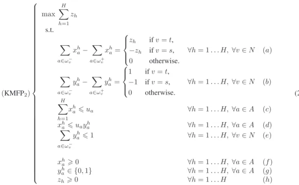
(KMFP2) max H X h=1 zh s.t. X a∈ω− v xh a− X a∈ω+v xh a = zh ifv = t, −zh ifv = s, 0 otherwise. ∀h = 1 . . . H, ∀v ∈ N (a) X a∈ω− v yh a− X a∈ω+ v yh a = 1 ifv = t, −1 if v = s, 0 otherwise. ∀h = 1 . . . H, ∀v ∈ N (b) H X h=1 xha 6ua ∀h = 1 . . . H, ∀a ∈ A (c) xh a 6uay h a ∀h = 1 . . . H, ∀a ∈ A (d) X a∈ω− v yh a 61 ∀h = 1 . . . H, ∀v ∈ N (e) xh a >0 ∀h = 1 . . . H, ∀a ∈ A (f ) yh a ∈ {0, 1} ∀h = 1 . . . H, ∀a ∈ A (g) zh>0 ∀h = 1 . . . H (h) (2)
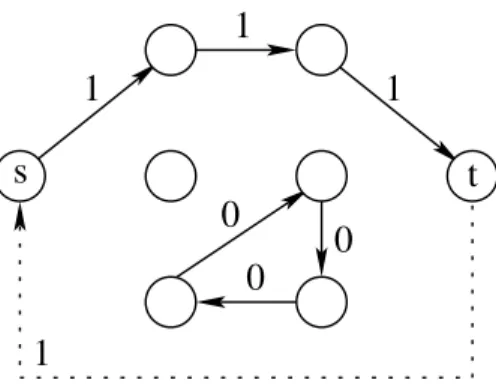
This model involves two flow conservation blocks (namely constraints2(a) and 2(b)) for each path.2(c) are the capacity constraints and 2(d) are the coupling constraints. Restrictions 2(e) are used to force each pathh to be elementary that is, to prevent cycles to be connected to the path. Otherwise, one could not prevent the flow bifurcation illustrated in figure 1. Arcsa correspond to decision variablesyha = 1 and, for each one, the flow value xha is reported. In such a situation, a cycle on path definition variablesyh may help define more than one flow path on variablesxh. Restrictions2(d) do not prevent disconnected cycles, as shown in figure 2. However, since such cycles cannot lead to flow bifurcation, this situation does not need to be forbidden.
1
1
1
1
s
t
1
1
1
1
1
1
0
0
0
2
s
t
1
1
1
0
1
0
0
s
t
Figure 2: impact of a disconnected cycle over the flow variablesxp.
2.3 Arc-path reformulation
By performing a Dantzig-Wolfe reformulation of model (KMFP2), a new arc-path model can be defined. It differs from model (KMFP1) since it relies on a discretization on decision and flow variables. Letxh
p >0 be the flow of path p when p is used as path number h. Let yhp ∈ {0, 1} be the corresponding decision variable. This new model is as follows:
(KMFP3) max H X h=1 X p∈P xhp s.t. H X h=1 X p∈P δapxhp ≤ ua ∀a ∈ A (a) xh p− upyph60 ∀h = 1 . . . H, ∀p ∈ P (b) X p∈P yph61 ∀h = 1 . . . H (c) xh p >0 ∀h = 1 . . . H, ∀p ∈ P (d) yph ∈ {0, 1} ∀h = 1 . . . H, ∀p ∈ P (e) (3)
When compared to model (KMFP1), model (KMFP3) does not need any restriction on the number of active paths anymore since it is implicitely assumed throught the variable discretization. However, an additional assignment step is required for the path variables, through constraints 3(c). Note that the solution of model (KMFP3) can always be translated into a solution of model (KMFP1) using the following formulas:
xp= H X h=1 xhp ∀p ∈ P (4) yp= max h=1...Hy h p ∀p ∈ P (5)
In fact, the relashionship between those two models is even stronger, as shown below:
Proof. Let (xh
p, yhp) be a fractional solution of model (KMFP3). Let xp = Phxhp and yp = P
hyhp be the aggregated variables. The solution(xp, yp) satisfies all the constraints of the model (KMFP1).
Let(xp, yp) be a fractional solution of model (KMFP1). Letxhp = xp/H and yph = yp/H be the disaggregated variables. The solution (xh
p, xhp) satisfies all the constraints of the model (KMFP3).
ThusConv(KMFP3) = Conv(KMFP1).
Now, when comparing to the model (KMFP2), the situation is different:
Property 2. Model (KMFP3) is stronger than model (KMFP2).
Proof. Let (xhp, yhp) be a fractional solution of model (KMFP3). Let xha = Ppδapxhp and yah = P
pδ p
ayhp be the projection on the arc variables. The solution(xha, yha) satisfies all the constraints of the model (KMFP2).
The reverse does not hold, as any flow on the arc variables may be decomposed into a set of elementary paths and elementary cycles (see Ahuja et al [1]). Thus, as the model (KMFP2) does not forbid cycles, many solutions from the model (KMFP2) cannot be translated into solutions from the model (KMFP3), see for instance the figure 2.
Therefore, the model (KMFP3) is stronger than the model (KMFP2).
2.4 Improvements
One obvious drawback of model (KMFP3) is its size. However, there is another one, closely related to the symmetry structure induced by the assignment of the decision variables [22]. Namely, assuming setP = (p1, p2, . . . , pH) is an optimal set of paths for model (KMFP3), any permutation ofP gives an optimal solution. As any path can be set at any position in the routing solution, it can potentially lead to a big number of “identical” solutions. One way to break this variable symmetry is to introduce the so-called variable-ordering constraints. In our situation, stating that the path in position h + 1 is required to have less flow than the path in position h is sufficient for most of the cases. However, this cannot break ties when, in the optimal solution, at least two paths carry the same amount of flow. The variable ordering is achieved through the following additional constraint: X p∈P xh+1p −X p∈P xhp 60 ∀h = 1 . . . H − 1 (6)
3
Branch and Price
One popular and efficient way to solve a MILP in extended formulation is to apply the branch and price scheme. It consists in embedding a column generation into a branch and bound framework. Branch and bound principle was presented by Land and Doig in [15]. Shortly before, Ford and Fulkerson ([10]) suggested column generation for multicommodity flow problem and Danzig and Wolfe ([9]) developed this idea in their well-known decomposition scheme. Finally, Barnhart et
al.[6] and Vanderbeck and Wolsey [23] described generic algorithms for solving problems by integer programming column generation. Many applications are presented in the literature, as can be seen in the survey of L ¨ubbecke and Desrosiers ([16]).
3.1 Column generation
The column generation is used to solve linear programs with a large number of variables (columns). It is based on the implicit knowledge of the whole setX of variables. At each iteration, it first solves a restricted master problem (RMP) and then solves a subproblem (SP) before updating the (RMP). The (RMP) consists in a restriction ofX to a feasible subset of variables S ⊂ X . Once the (RMP) has been solved to optimality onS, one has to check wether there exist improving variables inX \ S or not. This is done through the pricing procedure in (SP): using the dual information of the (RMP), the most violated reduced cost of a variable inX \ S is computed. If this reduced cost is improving, the associated variable is inserted into the (RMP) for subsequent iterations. Other-wise no improving variables exist, the column generation is stopped and the optimal solution of the (RMP) is the proven optimal solution of the problem.
In order to apply the branch and price technique on model (KMFP3), it is first continuous relaxed. Then, it is simplified using the following property:
Property 3. There is at least one optimal solution of the linear relaxation of (KMFP3) where the
coupling contraints are saturated.
Proof. Let(x∗, y∗) be an optimal solution. Let yh
p = xh∗p /up ifup > 0 and 0 otherwise, for each p in P and for each h = 1 . . . H. Then constraints 3(b) imply that yh
p 6yph∗, for eachp in P and for eachh = 1 . . . H. SoP
p∈Pyhp 6 P
p∈Pyh∗p 6 1 for each h = 1 . . . H (constraints 3(c)). Then(x∗
, y) is a feasible solution and provides the same value than (x∗ , y∗
). Therefore, (x∗ , y) is an optimal solution too.
Thus, coupling constraints can be dropped and the decision variablesy can be replaced with the flow variables x. This leads to a simplified version of the linear relaxation, including the variable-ordering constraints: (LR3) max H X h=1 X p∈P xhp s.t. H X h=1 X p∈P δapxhp 6ua ∀a ∈ A (a) X p∈P xh p up 61 ∀h = 1 . . . H (b) X p∈P xh+1p − X p∈P xhp 60 ∀h = 1 . . . H − 1 (c) xh p >0 ∀h = 1 . . . H ∀p ∈ P (c) (7)
Let respectivelyλa > 0, µh > 0 and νh > 0 be the dual variables associated to the primal constraints7(a), 7(b) and 7(c) of the linear relaxation (LR3). Then, the subproblem (SP) consists in finding a variable maximizing the reduced cost. (SP) can be decomposed intoH subproblems (SPh). Each of them reduces to an optimal cost elementary path problem for position h. The reduced cost is given by
ch p = 1 − X a∈A δapλa− µh up − (νh−1− νh) (8)
The computation of the maximal cost elementary path does not reduce to a simple shortest path problem, since the reduced cost involves a combination of two dual variables,λ and µ (the cost associated to the variable-ordering constraints only depend on the path position and not on the arcs of the path). Given a path positionh, the subproblem is as follows:
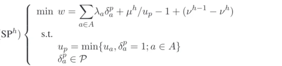
(SPh) min w =X a∈A λaδap+ µh/up− 1 + (νh−1− νh) s.t. up= min{ua, δap = 1; a ∈ A} δap ∈ P (9)
More precisely, for any optimal path problem, Martin [19] defined the weak optimality
prin-cipleas the fact that there is an optimal path made of optimal subpaths. He then showed that this principle is a necessary condition to the application of any labelling algorithm (for instance, the classical label setting / label correcting algorithms for the shortest path problem).
Unfortunately, our subproblem (SP) does not meet Martin’s weak optimality principle, as il-lustrated in figure 3. For each arca, the first number refers to its dual variables λawhile the second one refers to its capacityua. The variable µ is supposed to be set to 4. The shortest path from nodes to node v uses the arc a2 sinceλ1+ µ/c1 = 5 > λ2+ µ/c2 = 4. The shortest path from nodes to node t uses the path a2− a3sinceλ1+ λ3+ µ/c1 = 5 < λ2+ λ3+ µ/c3= 7.
a2[2; 2]
a1[1; 1]
a3[1; 1]
s v t
Figure 3: failure of the weak optimality principle
Thus, no labelling algorithm can be used to compute the optimal solution [19] and a specific algorithm has to be designed.
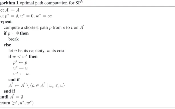
In(SPh), the variables δpadefine the pathp as they are the projection of variables ypover the arcs whileupdefines its capacity. The optimal pathp∗is a combination between the shortest path and the highest capacity path. Its computation can be done in the following way:
Property 4. Algorithm 1 runs in polynomial time
Proof. There is no negative cost arc since λa > 0, ∀a ∈ A. Thus, no negative cost cycle exists and any polynomial-time shortest path algorithm may be used. Next, at each iteration of the algorithm, at least one arc is removed from the setA′. Thus, there is at mostm iterations, that is m computations of a shortest path.
Since the columns might be used anywhere in the branching tree, they are inserted into a global pool. The column generation will stop as soon asw∗
60.
3.2 Classical branchings
Since the column generation works on the linear relaxation of the initial problem, one has to perform branchings. The classical branching scheme of Dakin [8] cannot be applied as it works
Algorithm 1 optimal path computation for SPh letA′ = A letp∗ = ∅, u∗ = 0, w∗ = ∞ repeat
compute a shortest pathp from s to t on A′
ifp = ∅ then break
else
letu be its capacity, w its cost
ifw < w∗ then p∗ ← p u∗ ← u w∗ ← w end if A′ ← A′ \ {a ∈ A′ | ua6u} end if untilA′ = ∅ return(p∗ , u∗ , w∗ )
on the original variables and as it is quite difficult to prevent the generation of a column that has already been forbidden in the current branch. Ryan and Foster [21] were among the first to propose a safe branching scheme ((x = y) ∨ (x 6= y)). Instead of forcing or forbidding a decision variable, their idea relies on the fact that either two variables are set the same way or not.
More recently, Barnhart et al. [5] proposed a more efficient branching for the routing problems. It is based on the concept of node of divergence over the aggregated flowxh
a =Ppδ p
axhp, ∀a ∈ A. A node of divergence is a noded ∈ N such that the aggregated flow is coming from a single arc and going out on several arcs, see figure 4. Given a positionh 6 H, a divergence occurs when the flow decision variablesyh
p are fractional. On figure 4, those fractions are respectively7/10, 1/10 and2/10. Thus, a fractional part of each path p is used.
7
10
1
7
2
2
s
d
t
Figure 4: divergence on aggregated flowxhon noded.
Letω+d be the cocycle of arcs going out of noded. Let ω1 and ω2 be a partition ofωv+such that each set contains at least one arc carrying a positive amount of flow. LetP1 ⊂ P and P2⊂ P be the set of paths going through noded and using one arc of respectively ω1 and ω2. Since the flow onxhhas to be integer (that is, unsplittable), either it uses one arc in the setω1or in the set ω2. Then the following branching is valid:
(X p∈P1 yhp = 0) vs. ( X p∈P2 yhp = 0)
For a better efficiency, the branching should be applied on the first node of divergence and the setsP1andP2should be built such that each sum is the most fractional.
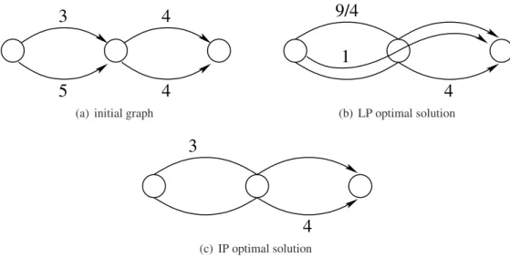
It can be noted that this kind of branching cannot be easily applied to the first model (KMFP1) as more than one path may be needed at the node of divergence. This situation is illustrated on figure 5. Figure 5(a) shows a graph whose capacities are reported. We wish to send the maximal amount of flow from s to t using at most H = 2 paths. Figure 5(b) illustrates the optimal relaxed solution. All the capacities are satisfied by the aggregated flow and the sum P
p∈Pyp =Pp∈Pxp/up = 3/4 + 1/4 + 1 = 2 satisfies the path limit H. Clearly, this solution uses three paths and no branching as defined previously can be done. The optimal integer solution is reported in figure 5(c).
3
4
4
5
(a) initial graph
4
1
9/4
(b) LP optimal solution3
4
(c) IP optimal solutionFigure 5: divergence on aggregated flowx on node d.
Three paths are currently using noded and the limit is set to 2. However, the optimal solution uses two paths atd and no arc partition may help converging towards this solution.
3.3 Alternate branching
One of the shortcoming of the previous branching scheme is that it might require a careful parti-tioning procedure in order to be efficient. And even then, its efficiency will come from a combina-tion of several successive branchings. We propose another branching scheme based on the number of path positions using an arc.
Leta ∈ A be an arc and S ⊂ Habe a subset of the path positions that usea. Then either all the path positions usea or at least one of them is not using a. More formaly, the branching is as follows: (X h∈S yha = |S|) vs. (X h∈S yha 6|S| − 1)
(X h∈S yah= |S|) ⇒ ( X h∈S X p∈P xhp 6ua)
There is no equivalence as a linear combination of several paths may be used to route the flow at any path position in the relaxed solution – not only one path. Thus, this restriction is stronger than the capacity contraint3(a):
X h∈S X p∈P δpaxhp 6X h∈S X p∈P xhp 6ua
When switching back to the variables on the arcs, this branch becomes: (X h∈S X p∈P xhp 6ua) ⇔ ( X h∈S X a′∈Ω+s xha′ 6ua)
The other branch is equivalent to state that at least one of those path position should not route anything ona. It can be reformulated as follows
(X
h∈S
yah6|S| − 1) ⇔ (∃h ∈ S | yha = 0)
If the subsetS is reduced to a single path position, then the branching looks somewhat simpler:
( X
a′∈Ω+ s
xha′ 6ua) vs. (yha = 0)
The branching can only be done if there is a path position h such that the fractional flow is routing more than the capacity of an arca used by h. Otherwise, a classical branching must be done. Even if the branching can be expressed in the arc-path formulation, it is better to use the node-arc formulation: as a branch leads to a new constraint in the RMP, a new dual variable will be added. This will alter the pricing subproblem and make it harder to solve. Thus, one solution is to use the node-arc formulation for the branching and link the node-arc variables with the arc-path variables. This is close to the Explicit Master formulation in the Robust Branch and Cut and Price (RBCP) proposed by Fukasawa et al. [11]. The RMP now looks like:
(LR4) max H X h=1 X p∈P xhp s.t. X p∈P δhaxhp − xha 60 ∀h = 1 . . . H, ∀a ∈ A (a) H X h=1 X p∈P δapxhp 6ua ∀a ∈ A (b) X p∈P xh p up 61 ∀h = 1 . . . H (c) xh p >0 ∀h = 1 . . . H ∀p ∈ P (d) xh a>0 ∀h = 1 . . . H ∀a ∈ A (e) (10)
Then the branching will be done on thexh
a variables while the column generation will work on thexh
3.4 Initialization
One crucial question that arises when implementing a column generation is the construction of the initial set of columns. For minimum cost flow problems, this may requires a carefull initialisation. The situation is different for the KMFP since even no path for each path position might lead to an initial feasible solution.
However, a better way to start is to compute an initial feasible solution, with respect to the width constraint. This can be done by using Baier et al. [4] approximation algorithm. It is based on an iterative insertion of a new path into the solution:
Algorithm 2 approximation algorithm for the KMFP
letqabe the number of paths using arca, initialy qa← 0 letP be the set of paths, initialy P ← ∅
letf be the flow carried by each path, initialy f ← 0
repeat
letG′
= (N, A′
) be the residual graph with capacities ca= ua/(1 + qa) backward arcs have capacitiesca= f
compute a max capacity pathp from s to t on G′ letc be its capacity
updateP : P ← P ∪ {p}
for all backward arca ∈ p do
updatep and a path p′ ∈ P using arc a (deviation)
end for
updatef : f ← c for each path
untilp = ∅ or |P | = H return(P, f )
This algorithm runs in polynomial time. The setP of paths can then be used as the initial set of columns.
4
Numerical results
4.1 Instances
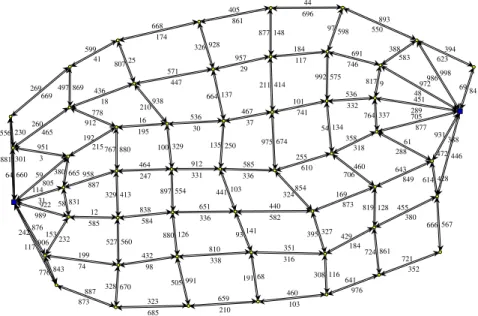
Two kinds of instances have been used to run our experiments. The first set of instances has been generated by the Transit Grid generator developped by G. Waissi1. The topology of those instances (see figure 6) looks close to the transportation networks and may be well-suited for studying the maxflow problem in the telecommunication networks as well. The second kind of topology in completely randomly generated: the edges are randomly chosen so as to have a con-nected network and the capacity of those edges is randomly chosen.
1http://www.informatik.uni-trier.de/∼naeher/Professur/research/generators/
301 660 805 31 989 242 117 873 843 906 74 232 776 876 585 831 153 922 887 665 58 114 215 951 380 59 465 230 3 64 669 556 881 685 670 887 98 560 328 199 584 413 527 12 247 880 329 958 195 778 767 192 18 869 912 260 41 497 269 210 991 323 338 126 505 432 336 554 880 838 331 329 897 464 30 938 100 16 447 25 210 436 174 807 599 103 68 659 316 141 191 810 582 103 93 651 336 250 441 912 37 137 135 536 29 928 664 571 861 326 668 976 116 460 184 327 308 351 873 854 395 440 610 674 324 585 741 414 975 467 117 148 211 957 696 877 405 352 861 641 380 128 724 429 849 460 819 169 318 134 706 255 332 575 54 101 746 598 992 184 550 97 44 567 721 446 428 666 455 388 61 614 643 877 337 288 358 289 9 764 536 48 583 817 691 986 623 388 893 69 394 84 998 972 451 705 931 472 s t
Figure 6: transit grid with 52 nodes and 198 arcs.
4.2 Results
The experiments were done on a Pentium 4 computer with 4Gb memory. The time limit has been set to 1 hour for each run.
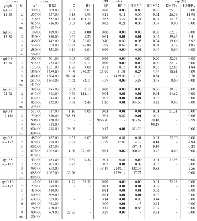
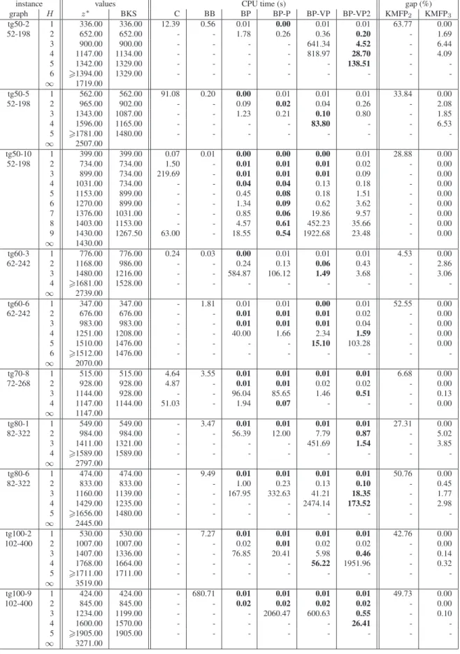
For each table (table 1 to table 5) the column “Graph” gives the name of the instance, along with the number of nodes and the number of arcs. The width upper limit H is reported in the second column. The columnz∗
gives the optimal value, whenever available by at least one of our algorithms in the time limit. Otherwise, the sign “>” shows only a lower bound is known (the best integer found so far). The value of the solution obtained by the algorithm from Baier, K ¨olher et Skutella [4] is reported in column “BKS”. As the CPU time is marginal compared to the other strategies, it is not reported.
Table 1 to table 3 report the CPU time of several strategies. Those strategies are:
C : the arc-node model (KMFP2) is solved using CPLEX 8.0
BB : the arc-node model (KMFP2) is solved using Barnhart’s branching in a home-made branch and bound
BP : the extended model (KMFP3) is solved using Barnhart’s branching in a home-made branch and price
BP-V : similar to BP, except that the global pool strategy is used BP-VP : similar to BP-V, except that the variable ordering is used BP-VP2 : similar to BP-VP, except that the alternate branching is used
In the last two columns, we give the root gap from both the arc-node (KMFP2) model and from the extended (KMFP3) model. Thus the root gap stands for the relative gap between the fractional solution and the integer solution of the problem.
We can note that the gap is a lot better for the extended model. This is closely related to the problem with the subcycles illustrated in the figure 1: by relaxing the binary variables, the fractional solution may have some cycles on the flow definition variables yah, for fixed values of h. Those cycles will help artificialy improve the amount of flow that can be routed. The extended model relies on elementary paths. Its fractional solution could create cycles on the path definition variablesyph, for fixed values ofh. However, as the flow variables xhp are on the path too, no artificial improvement can be done. As the extended model has a smaller root gap than the arc-node model, this will explain why the “BP*” strategies always dominate the “C” and “BB” approaches in term of CPU time.
instance values CPU time (s) gap (%)
graph H z∗ BKS C BB BP BP-P BP-VP BP-VP2 KMFP2 KMFP3 tg10-2 1 389.00 389.00 0.01 0.01 0.00 0.00 0.00 0.00 25.13 0.00 12-38 2 557.00 557.00 0.18 0.93 0.21 0.11 0.06 0.02 26.59 11.98 3 716.00 557.00 1.44 104.74 9.65 4.27 0.21 0.02 12.15 6.18 4 815.00 716.00 0.03 7.48 0.02 0.21 0.06 0.07 0.00 0.00 ∞ 815.00 tg10-3 1 189.00 189.00 0.02 0.00 0.00 0.00 0.00 0.00 52.13 0.00 12-38 2 350.00 350.00 0.51 0.25 0.01 0.01 0.01 0.02 39.66 3.41 3 466.00 442.00 3.04 21.82 0.40 0.09 0.05 0.04 19.66 6.92 4 558.00 558.00 70.97 586.99 2.98 0.69 0.12 0.07 3.79 1.95 5 580.00 558.00 0.11 0.04 0.00 0.00 0.01 0.04 0.00 0.00 ∞ 580.00 tg10-9 1 501.00 501.00 0.03 0.01 0.00 0.00 0.00 0.00 32.58 0.00 12-38 2 935.00 935.00 0.23 0.11 0.00 0.00 0.00 0.00 32.77 0.00 3 1173.00 1051.00 1.95 9.08 0.51 0.15 0.06 0.05 22.68 1.84 4 1356.00 1289.00 13.09 930.27 21.99 11.51 0.23 3.46 10.61 4.09 5 1460.00 1364.00 288.64 - - 1419.06 11.29 0.54 - 2.78 6 1517.00 1364.00 5.52 82.11 3.57 0.09 5.88 0.68 0.00 0.00 ∞ 1517.00 tg20-2 1 385.00 385.00 0.02 0.13 0.00 0.00 0.00 0.00 18.43 0.00 22-72 2 643.00 643.00 0.38 112.14 0.01 0.01 0.01 0.01 24.62 0.00 3 832.00 643.00 1.94 - 0.05 0.01 0.01 0.05 - 0.00 4 853.00 832.00 0.38 2.43 1.26 0.01 104.60 0.22 0.00 0.00 ∞ 853.00 tg40-1 1 517.00 517.00 1.16 0.05 0.01 0.01 0.01 0.01 21.31 0.00 42-152 2 750.00 520.00 788.84 - 0.04 0.02 0.01 0.04 - 0.06 3 908.00 750.00 - - 2066.70 - 303.87 20.18 - 2.59 4 994.00 918.00 - - - 90.29 - -5 1004.00 918.00 28.09 - 0.17 0.01 183.20 - - 0.00 ∞ 1004.00 tg40-5 1 487.00 487.00 0.23 0.07 0.00 0.01 0.01 0.01 22.70 0.00 42-152 2 828.00 828.00 2.87 - 23.29 17.87 4.19 0.14 - 4.94 3 1062.00 828.00 - - - - 137.41 0.36 - 0.28 4 1078.00 1062.00 11.88 271.55 0.02 0.02 100.26 0.98 0.00 0.00 ∞ 1078.00 tg40-8 1 454.00 454.00 0.31 0.52 0.01 0.01 0.00 0.01 27.93 0.00 42-152 2 775.00 705.00 16.42 - 0.05 0.01 0.02 0.03 - 0.00 3 991.00 858.00 - - 1138.19 2148.15 332.33 0.85 - 2.56 4 1085.00 1067.00 32.26 - - 1739.14 17.72 - - 0.00 ∞ 1085.00 tg40-10 1 142.00 142.00 1.71 26.32 0.00 0.00 0.00 0.01 72.28 0.00 42-152 2 278.00 278.00 - - 0.01 0.01 0.01 0.02 - 0.00 3 410.00 410.00 - - 0.01 0.01 0.01 0.02 - 0.00 4 509.00 509.00 - - 0.01 0.01 0.01 0.03 - 0.00 5 602.00 553.00 - - 0.14 0.01 0.88 0.44 - 0.00 6 691.00 642.00 - - 0.06 0.01 1.43 0.91 - 0.00 7 769.00 720.00 - - 0.17 0.01 0.63 2.07 - 0.00 8 804.00 769.00 22.75 - 0.29 0.09 - 9.21 - 0.00 ∞ 804.00
instance values CPU time (s) gap (%) graph H z∗ BKS C BB BP BP-P BP-VP BP-VP2 KMFP2 KMFP3 tg50-2 1 336.00 336.00 12.39 0.56 0.01 0.00 0.01 0.01 63.77 0.00 52-198 2 652.00 652.00 - - 1.78 0.26 0.36 0.20 - 1.69 3 900.00 900.00 - - - - 641.34 4.52 - 6.44 4 1147.00 1134.00 - - - - 818.97 28.70 - 4.09 5 1342.00 1329.00 - - - 138.51 - -6 >1394.00 1329.00 - - - -∞ 1719.00 tg50-5 1 562.00 562.00 91.08 0.20 0.00 0.01 0.01 0.01 33.84 0.00 52-198 2 965.00 902.00 - - 0.09 0.02 0.04 0.26 - 2.08 3 1343.00 1087.00 - - 1.23 0.21 0.10 0.80 - 1.85 4 1596.00 1165.00 - - - - 83.80 - - 6.53 5 >1781.00 1480.00 - - - -∞ 2507.00 tg50-10 1 399.00 399.00 0.07 0.01 0.00 0.00 0.00 0.01 28.88 0.00 52-198 2 734.00 734.00 1.50 - 0.01 0.01 0.01 0.02 - 0.00 3 899.00 734.00 219.69 - 0.01 0.01 0.01 0.09 - 0.00 4 1031.00 734.00 - - 0.04 0.04 0.13 0.18 - 0.00 5 1153.00 899.00 - - 0.45 0.08 0.18 1.51 - 0.00 6 1270.00 899.00 - - 1.34 0.09 0.62 3.62 - 0.00 7 1376.00 1031.00 - - 0.85 0.06 19.86 9.57 - 0.00 8 1403.00 1153.00 - - 4.57 0.61 452.23 35.66 - 0.00 9 1430.00 1267.50 63.00 - 18.55 0.54 1922.68 23.48 - 0.00 ∞ 1430.00 tg60-3 1 776.00 776.00 0.24 0.03 0.00 0.01 0.01 0.01 4.53 0.00 62-242 2 1168.00 986.00 - - 0.24 0.13 0.06 0.43 - 2.86 3 1480.00 1216.00 - - 584.87 106.12 1.49 3.68 - 3.06 4 >1681.00 1528.00 - - - -∞ 2739.00 tg60-6 1 347.00 347.00 - 1.81 0.01 0.01 0.00 0.01 52.55 0.00 62-242 2 676.00 676.00 - - 0.01 0.01 0.01 0.02 - 0.00 3 983.00 983.00 - - 0.01 0.01 0.01 0.04 - 0.00 4 1251.00 1208.00 - - 40.00 1.66 2.34 1.59 - 0.00 5 1510.00 1476.00 - - - - 15.10 103.28 - 0.00 6 >1512.00 1476.00 - - - -∞ 2070.00 tg70-8 1 515.00 515.00 4.64 3.55 0.01 0.01 0.01 0.01 6.68 0.00 72-268 2 928.00 928.00 4.87 - 0.01 0.01 0.02 0.02 - 0.00 3 1144.00 928.00 - - 96.04 85.65 1.46 0.51 - 0.13 4 1147.00 1144.00 51.03 - 1.94 0.07 - - - 0.00 ∞ 1147.00 tg80-1 1 549.00 549.00 - 3.47 0.01 0.01 0.01 0.01 27.31 0.00 82-322 2 984.00 984.00 - - 56.39 12.00 7.79 0.87 - 5.02 3 1411.00 1321.00 - - - - 451.69 1.54 - 3.85 4 >1589.00 1589.00 - - - -∞ 2797.00 tg80-6 1 474.00 474.00 - 9.49 0.01 0.01 0.01 0.01 50.76 0.00 82-322 2 833.00 833.00 - - 1.00 0.23 0.13 0.10 - 0.45 3 1160.00 1139.00 - - 167.95 332.63 41.21 18.35 - 1.77 4 1429.00 1235.00 - - - - 2474.14 173.52 - 2.98 5 >1656.00 1480.00 - - - -∞ 2445.00 tg100-2 1 530.00 530.00 - 7.27 0.01 0.01 0.01 0.01 42.76 0.00 102-400 2 1007.00 1007.00 - - 0.02 0.01 0.02 0.02 - 0.00 3 1407.00 1336.00 - - 76.85 20.41 5.98 0.46 - 0.14 4 1768.00 1664.00 - - - - 56.22 1951.96 - 0.32 5 >1711.00 1711.00 - - - -∞ 3519.00 tg100-9 1 424.00 424.00 - 680.71 0.01 0.01 0.01 0.01 49.73 0.00 102-400 2 845.00 845.00 - - 0.02 0.02 0.02 0.02 - 0.00 3 1234.00 1199.00 - - - 2060.47 600.63 0.55 - 0.10 4 1600.00 1570.00 - - - 26.41 - -5 >1905.00 1905.00 - - - -∞ 3271.00
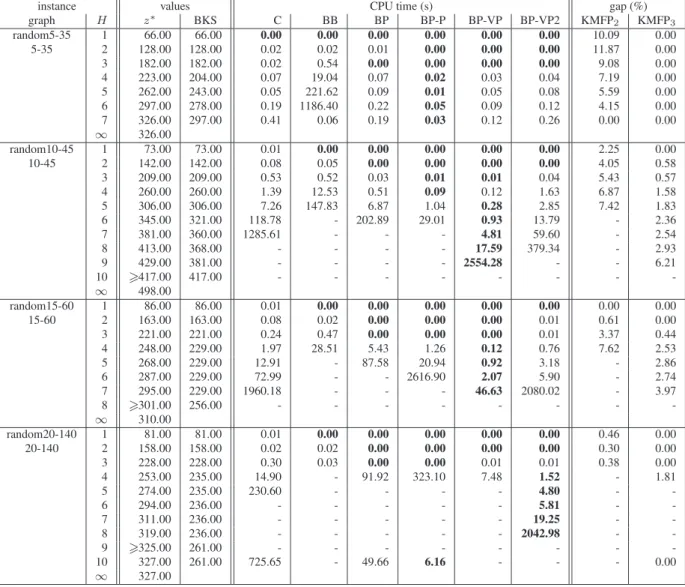
instance values CPU time (s) gap (%) graph H z∗ BKS C BB BP BP-P BP-VP BP-VP2 KMFP2 KMFP3 random5-35 1 66.00 66.00 0.00 0.00 0.00 0.00 0.00 0.00 10.09 0.00 5-35 2 128.00 128.00 0.02 0.02 0.01 0.00 0.00 0.00 11.87 0.00 3 182.00 182.00 0.02 0.54 0.00 0.00 0.00 0.00 9.08 0.00 4 223.00 204.00 0.07 19.04 0.07 0.02 0.03 0.04 7.19 0.00 5 262.00 243.00 0.05 221.62 0.09 0.01 0.05 0.08 5.59 0.00 6 297.00 278.00 0.19 1186.40 0.22 0.05 0.09 0.12 4.15 0.00 7 326.00 297.00 0.41 0.06 0.19 0.03 0.12 0.26 0.00 0.00 ∞ 326.00 random10-45 1 73.00 73.00 0.01 0.00 0.00 0.00 0.00 0.00 2.25 0.00 10-45 2 142.00 142.00 0.08 0.05 0.00 0.00 0.00 0.00 4.05 0.58 3 209.00 209.00 0.53 0.52 0.03 0.01 0.01 0.04 5.43 0.57 4 260.00 260.00 1.39 12.53 0.51 0.09 0.12 1.63 6.87 1.58 5 306.00 306.00 7.26 147.83 6.87 1.04 0.28 2.85 7.42 1.83 6 345.00 321.00 118.78 - 202.89 29.01 0.93 13.79 - 2.36 7 381.00 360.00 1285.61 - - - 4.81 59.60 - 2.54 8 413.00 368.00 - - - - 17.59 379.34 - 2.93 9 429.00 381.00 - - - - 2554.28 - - 6.21 10 >417.00 417.00 - - - -∞ 498.00 random15-60 1 86.00 86.00 0.01 0.00 0.00 0.00 0.00 0.00 0.00 0.00 15-60 2 163.00 163.00 0.08 0.02 0.00 0.00 0.00 0.01 0.61 0.00 3 221.00 221.00 0.24 0.47 0.00 0.00 0.00 0.01 3.37 0.44 4 248.00 229.00 1.97 28.51 5.43 1.26 0.12 0.76 7.62 2.53 5 268.00 229.00 12.91 - 87.58 20.94 0.92 3.18 - 2.86 6 287.00 229.00 72.99 - - 2616.90 2.07 5.90 - 2.74 7 295.00 229.00 1960.18 - - - 46.63 2080.02 - 3.97 8 >301.00 256.00 - - - -∞ 310.00 random20-140 1 81.00 81.00 0.01 0.00 0.00 0.00 0.00 0.00 0.46 0.00 20-140 2 158.00 158.00 0.02 0.02 0.00 0.00 0.00 0.00 0.30 0.00 3 228.00 228.00 0.30 0.03 0.00 0.00 0.01 0.01 0.38 0.00 4 253.00 235.00 14.90 - 91.92 323.10 7.48 1.52 - 1.81 5 274.00 235.00 230.60 - - - - 4.80 - -6 294.00 236.00 - - - 5.81 - -7 311.00 236.00 - - - 19.25 - -8 319.00 236.00 - - - 2042.98 - -9 >325.00 261.00 - - - -10 327.00 261.00 725.65 - 49.66 6.16 - - - 0.00 ∞ 327.00
Table 3: CPU times for random digraphs.
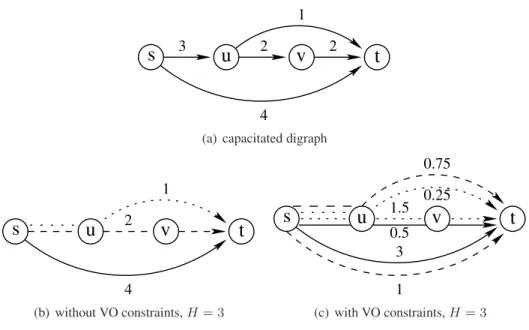
As a general point of view, the CPU time is decreasing when the strategy is improving (branch and price, adding the global pool, adding the variable ordering and using the alternate branching). However, on some instances, the strategies using the variable ordering seem to take a lot of time. This is especialy true when the width limitH is set to the maximal flow width (e.g. the width constraint becomes redundant). This may be explained by the dual variablesνhassociated to the variable ordering constraints. By the complementary slackness theorem, using theνhvariables in the dual solution implies the associated variable ordering constraints are saturated. This means two successive paths positions will route the same amount of flow. In order to have the same amount of flow, the fractional primal solution might have to use several paths for those path positions. Then, the fractional solution when using variable ordering constraints is more likely to be more “splitted” than without those contraints. This phenomenon is illustrated in figure 7. The fractional solution 7(b) without VO constraints is using 3 path positions, routing respectively 4, 2 and 1 unit of flow on a single path. When using VO contraints, the fractional solution 7(c) still uses 3 positions, routing respectively 4.5, 1.75 and 1.75 units of flow. However, each position is now using 2 paths
3 1 4 2 2
s
u
v
t
(a) capacitated digraph
1 4 2
s
u
v
t
(b) without VO constraints, H = 3 1.5 1 0.5 3 0.75 0.25s
u
v
t
(c) with VO constraints, H = 3Figure 7: impact of the VO constraints on the fractional solution.
Tables 4 to 6 will help us further analyse the problem. For each instance, we report the rate of nodes in the branch and bound tree whose fractional solution saturates at least one VO contraint. This rate is a lot higher when using the VO contraints.
instances values VO saturation (%) graph H z∗ BP-P BP-VP BP-VP2 tg10-2 1 389.00 0.00 0.00 0.00 12-40 2 557.00 0.29 23.15 41.18 3 716.00 0.04 65.53 71.43 4 815.00 1.68 84.85 75.00 ∞ 815.00 tg10-3 1 189.00 0.00 0.00 0.00 12-40 2 350.00 0.00 58.82 40.00 3 466.00 0.00 67.23 61.76 4 558.00 0.00 77.25 84.44 5 580.00 0.00 92.31 95.83 ∞ 580.00 tg10-9 1 501.00 0.00 0.00 0.00 12-40 2 935.00 0.00 0.00 100.00 3 1173.00 0.76 71.79 74.19 4 1356.00 0.30 74.60 81.08 5 1460.00 1.09 89.79 94.63 6 1517.00 1.00 99.98 96.23 ∞ 1517.00 tg20-2 1 385.00 0.00 0.00 0.00 22-80 2 643.00 0.00 0.00 100.00 3 832.00 0.00 0.00 54.55 4 853.00 0.00 79.04 86.49 ∞ 853.00 tg40-1 1 517.00 0.00 0.00 0.00 42-160 2 750.00 0.00 50.00 22.22 3 908.00 0.12 10.91 28.37 4 994.00 0.61 78.07 39.55 5 1004.00 0.00 99.23 65.01 ∞ 1004.00 tg40-5 1 487.00 0.00 0.00 0.00 42-160 2 828.00 0.30 20.54 45.16 3 1062.00 0.06 88.34 59.62 4 1078.00 0.00 99.68 70.75 ∞ 1078.00 tg40-8 1 454.00 0.00 0.00 0.00 42-160 2 775.00 0.00 0.00 25.00 3 991.00 0.28 27.36 34.67 4 1085.00 0.43 96.09 75.41 ∞ 1085.00 tg40-10 1 142.00 0.00 0.00 0.00 42-160 2 278.00 0.00 0.00 100.00 3 410.00 0.00 100.00 0.00 4 509.00 0.00 100.00 100.00 5 602.00 0.00 98.82 94.87 6 691.00 0.00 99.63 94.29 7 769.00 0.00 99.44 99.07 8 804.00 3.03 100.00 83.60 ∞ 804.00
instances values VO saturation (%) graph H z∗ BP-P BP-VP BP-VP2 tg50-2 1 336.00 0.00 0.00 0.00 52-200 2 652.00 3.97 42.18 66.67 3 900.00 1.81 81.08 69.54 4 1147.00 0.47 90.73 86.72 5 1342.00 1.71 97.17 87.22 6 >1394.00 1.20 97.75 91.94 ∞ 1719.00 tg50-5 1 562.00 0.00 0.00 0.00 52-200 2 965.00 0.00 34.48 40.00 3 1343.00 4.20 60.00 64.00 4 1596.00 4.15 74.54 67.20 5 >1781.00 1.14 94.92 74.61 ∞ 2507.00 tg50-10 1 399.00 0.00 0.00 0.00 52-200 2 734.00 0.00 0.00 100.00 3 899.00 0.00 0.00 87.50 4 1031.00 12.50 89.86 81.25 5 1153.00 0.00 75.00 48.75 6 1270.00 7.89 84.79 26.06 7 1376.00 21.05 80.54 33.90 8 1403.00 0.94 99.81 51.40 9 1430.00 21.73 98.53 98.22 ∞ 1430.00 tg60-3 1 776.00 0.00 0.00 0.00 62-240 2 1168.00 0.00 26.09 40.48 3 1480.00 0.06 31.54 48.05 4 >1681.00 0.21 65.70 3.89 ∞ 2739.00 tg60-6 1 347.00 0.00 0.00 0.00 62-240 2 676.00 0.00 0.00 100.00 3 983.00 0.00 0.00 100.00 4 1251.00 3.48 84.70 36.90 5 1510.00 3.92 57.07 17.75 6 >1512.00 5.08 96.67 15.81 ∞ 2070.00 tg70-8 1 515.00 0.00 0.00 0.00 72-280 2 928.00 0.00 0.00 100.00 3 1144.00 0.00 6.53 16.00 4 1147.00 0.00 91.70 53.60 ∞ 1147.00 tg80-1 1 549.00 0.00 0.00 0.00 82-320 2 984.00 0.00 18.94 46.24 3 1411.00 0.24 75.57 46.43 4 >1589.00 1.99 93.54 91.87 ∞ 2797.00 tg80-6 1 474.00 0.00 0.00 0.00 82-320 2 833.00 0.00 19.30 40.00 3 1160.00 0.52 33.12 18.95 4 1429.00 1.46 81.85 46.63 5 >1656.00 4.40 84.30 84.65 ∞ 2445.00 tg100-2 1 530.00 0.00 0.00 0.00 102-400 2 1007.00 0.00 0.00 100.00 3 1407.00 0.03 27.02 52.38 4 1768.00 0.58 38.91 20.22 5 >1711.00 2.95 90.15 74.36 ∞ 3519.00 tg100-9 1 424.00 0.00 0.00 0.00 102-400 2 845.00 0.00 0.00 100.00 3 1234.00 2.95 44.71 62.86 4 1600.00 2.11 80.51 75.45 5 >1905.00 7.60 95.20 56.36 ∞ 3271.00
instances values VO saturation (%) graph H z∗ BP-P BP-VP BP-VP2 random5-35 1 66.00 0.00 0.00 0.00 5-35 2 128.00 0.00 0.00 100.00 3 182.00 0.00 100.00 0.00 4 223.00 18.52 82.98 87.50 5 262.00 0.00 94.03 90.38 6 297.00 14.10 93.14 90.48 7 326.00 17.14 98.36 94.21 ∞ 326.00 random10-45 1 73.00 0.00 0.00 0.00 10-45 2 142.00 0.00 100.00 0.00 3 209.00 34.48 88.24 92.31 4 260.00 12.56 94.58 94.59 5 306.00 12.62 98.11 98.22 6 345.00 10.05 98.37 98.23 7 381.00 9.45 99.57 98.63 8 413.00 9.91 99.48 99.29 9 429.00 13.79 99.78 98.98 10 >417.00 99.85 ∞ 498.00 random15-60 1 86.00 0.00 0.00 0.00 15-60 2 163.00 0.00 0.00 100.00 3 221.00 0.00 100.00 0.00 4 248.00 0.95 67.27 89.11 5 268.00 2.33 91.93 95.74 6 287.00 4.14 99.38 98.87 7 295.00 6.25 97.75 90.46 8 >301.00 7.66 99.26 97.39 9 >306.00 11.43 99.98 98.43 10 310.00 13.04 100.00 99.99 ∞ 310.00 random20-140 1 81.00 0.00 0.00 0.00 20-140 2 158.00 0.00 0.00 100.00 3 228.00 0.00 100.00 100.00 4 253.00 2.10 69.25 83.81 5 274.00 2.47 73.09 94.70 6 294.00 25.74 99.96 95.67 7 311.00 12.14 99.99 98.34 8 319.00 13.57 97.92 96.49 9 >319.00 13.54 99.58 99.79 10 327.00 19.70 100.00 99.98 ∞ 327.00
Table 6: saturation on VO constraints for random digraphs.
5
Conclusion
The extended model (KMFP3) has a clear advantage over the arc-node model (KMFP2) as the root gap is much lower. Thus the branch and price may seem to be the best way to solve the problem. From our experiment, we were able to solve medium-sized instances for a limited widthH. As H increases, the problem becomes harder to solve, until the width of the unrestricted maximum flow is reached. From a practical point of view, this is not really an issue as Internet Providers wish to work with small values – through the use of MPLS-TE for instance. Nevertheless, from a theoretical point of view, we believe our branch and price is limited by two factors: first, a lot of perturbations are introduced into the fractional solutions by the addition of VO constraints. As it was shown, the fractional solutions are using more paths for each path position. Therefore, more branchings need to be done to reach the integer solution. An alternate VO strategy that does not lead to such situation would really help the branch and price. Second, the two branching strategies shown in this work are lacking some efficiency. It would be interesting to find a stronger branching scheme, and maybe add some cuts in the LR4 model as in the RBCP strategy. We are currently
working on both issues.
References
[1] Ravindra K. Ahuja, Thomas L. Magnanti, and James B. Orlin. Network Flows - Theory,
Algorithms, and Applications. Prentice Hall, 1993.
[2] Filipe Alvelos and Jos´e Manuel Vasconcelos Val´erio de Carvalho. Comparing Branch-and-price Algorithms for the Unsplittable Multicommodity Flow Problem. In Proceedings of the
International Network Optimization Conference, pages 7–12, 2003.
[3] Alper Atamt¨urk and Deepak Rajan. On splittable and unsplittable capacitated network design arc-set polyhedra. Mathematical Programming, 92:315–333, 2002.
[4] Georg Baier, Ekkehard K ¨ohler, and Martin Skutella. On the k-splittable flow problem. In Proceedings of the 10th Annual European Symposium on Algorithms, pages 101–113. Springer-Verlag, 2002.
[5] Cynthia Barnhart, Christopher A. Hane, and Pamela H. Vance. Using branch-and-price-and-cut to solve origin-destination integer multicommodity flow problems. Operations Research, 48(2):318–326, 2000.
[6] Cynthia Barnhart, Ellis L. Johnson, George L. Nemhauser, Martin W.P. Savelsbergh, and Pamela H. Vance. Branch-and-price: column generation for solving huge integer programs.
Operations Research, 46:316–329, 1998.
[7] James E. Burns, Teunis J. Ott, Johan M. de Kock, and Anthony E. Krzesinski. Path Selection and Bandwidth Allocation in MPLS Networks: a Non-Linear Programming Approach. In
ITCom Conference, 2001.
[8] Robert J. Dakin. A tree-search algorithm for mixed integer programming problems. The
Computer Journal, 8(3):250–254, 1965.
[9] George B. Dantzig and Philip Wolfe. Decomposition principle for linear programs.
Opera-tions Research, 8:101–111, 1960.
[10] Lester R. Ford and Delbert R. Fulkerson. A suggested computation for maximal multicom-modity network flow. Management Science, 5:97–101, 1958.
[11] R. Fukasawa, M. Poggi de Aragao, O. Porto, and E. Uchoa. Robust branch-and-cut-and-price for the capacitated vehicle routing problem. In INOC Conference, pages 231–236, 2003. [12] Jon M. Kleinberg. Approximation algorithms for disjoint paths problems. PhD thesis,
Mas-sachusetts Institute of Technology, Dept. of Electrical Engineering and Computer Science, 1996.
[13] Ronald Koch, Martin Skutella, and Ines Spenke. Approximation and complexity of k-splittable flows. In WAOA, pages 244–257, 2005.
[14] Stavros Kolliopoulos. Minimum-cost single-source 2-splittable flow. Information Processing
Letters, 94:15–18, 2005.
[15] A. Land and A. Doig. An automatic method of solving discrete programming problems.
[16] Marco E. L ¨ubbecke and Jacques Desrosiers. Selected topics in column generation.
Opera-tions Research, 53(6):1007–1023, 2005.
[17] Maren Martens and Martin Skutella. Flows on Few Paths: Algorithms and Lower Bounds. In proceedings of ESA 2004, pages 520–531, 2004.
[18] Maren Martens and Martin Skutella. Length-Bounded and Dynamic k-Splittable Flows. In
proceedings of the International Scientific Annual Conference Operations Research, 2005. [19] Ernesto Martins. The optimal path problem. Investigac¸ ˜ao Operacional, 19:43–60, 1999. [20] Vahab S. Mirrokni, Marina Thottan, Huseyin Uzunalioglu, and Sanjoy Paul. A Simple
Poly-nomial Time Framework To Reduced Path Decomposition in Multi-Path Routing. In
pro-ceedings of INFOCOM 2004, 2004.
[21] David M. Ryan and Brian A. Foster. An integer programming approach to scheduling. In Anthony Wren, editor, Computer Scheduling of Public Transport : Urban Passenger Vehicle
and Crew Scheduling, pages 269–280. North-Holland Publishing Company, 1981.
[22] Hanif D. Sherali and J. Cole Smith. Improving discrete model representations via symmetry considerations. Management Science, 47(10):1396–1407, 2001.
[23] Franc¸ois Vanderbeck and Laurence A. Wolsey. An exact algorithm for ip column generation.
Operations Research Letters, 19(4):151–159, 1996.
[24] B´en´edicte Vatinlen. Optimisation du routage dans les r´eseaux de t´el´ecommunication avec