HAL Id: hal-00906168
https://hal.sorbonne-universite.fr/hal-00906168
Submitted on 19 Nov 2013
HAL is a multi-disciplinary open access
archive for the deposit and dissemination of sci-entific research documents, whether they are pub-lished or not. The documents may come from teaching and research institutions in France or abroad, or from public or private research centers.
L’archive ouverte pluridisciplinaire HAL, est destinée au dépôt et à la diffusion de documents scientifiques de niveau recherche, publiés ou non, émanant des établissements d’enseignement et de recherche français ou étrangers, des laboratoires publics ou privés.
Derivation of a Hele-Shaw type system from a cell model
with active motion
Benoît Perthame, Fernando Quirós, Min Tang, Nicolas Vauchelet
To cite this version:
Benoît Perthame, Fernando Quirós, Min Tang, Nicolas Vauchelet. Derivation of a Hele-Shaw type system from a cell model with active motion. Interfaces and Free Boundaries, European Mathematical Society, 2014, 14 (4), pp.489-508. �10.4171/IFB/327�. �hal-00906168�
Derivation of a Hele-Shaw type system from a cell model with
active motion
Benoˆıt Perthame∗† Fernando Quir´os‡ Min Tang§ Nicolas Vauchelet∗†
July 4, 2013
Abstract
We formulate a Hele-Shaw type free boundary problem for a tumor growing under the combined effects of pressure forces, cell multiplication and active motion, the latter being the novelty of the present paper. This new ingredient is considered here as a standard diffusion process. The free boundary model is derived from a description at the cell level using the asymptotic of a stiff pressure limit.
Compared to the case when active motion is neglected, the pressure satisfies the same comple-mentarity Hele-Shaw type formula. However, the cell density is smoother (Lipschitz continuous), while there is a deep change in the free boundary velocity, which is no longer given by the gradient of the pressure, because some kind of ‘mushy region’ prepares the tumor invasion.
Key-words: Tumor growth; Hele-Shaw equation; porous medium equation; free boundary problems. Mathematics Subject Classification35K55; 35B25; 76D27; 92C50.
1
Introduction
Among the several models now available to deal with cancer development, there is a class, initiated in the 70’s by Greenspan [15], that considers that cancerous cells multiplication is limited by nutrients (glucosis, oxygen) brought by blood vessels. Models of this class rely on two kinds of descriptions; either they describe the dynamics of cell population density [5] or they consider the ‘geometric’ motion of the tumor through a free boundary problem; see [11,10,13,16] and the references therein. In the latter kind of models the stability or instability of the free boundary is an important issue that has attracted attention, [9,13].
The first stage, where growth is limited by nutrients, lasts until the tumor reaches the size of ≈ 1mm; then, lack of food leads to cell necrosis which triggers neovasculatures development [8] that supply the tumor with enough nourishment. This has motivated a new generation of models where growth
∗UPMC Univ Paris 06 and CNRS UMR 7598, Laboratoire Jacques-Louis Lions, F-75005, Paris, France. Email B. P.:
[email protected], Email N. V.: [email protected]
†
INRIA Paris Rocquencourt EPC BANG. France.
‡
Departamento de Matem´aticas, Universidad Aut´onoma de Madrid, 28049-Madrid, Spain. Supported by Spanish project MTM2011-24696. Email: [email protected]
§
Department of mathematics, Institute of Natural Sciences and MOE-LSC. Shanghai Jiao Tong University, China. Email: [email protected]
is limited by the competition for space [4], turning the modeling effort towards mechanical concepts, considering tissues as multiphasic fluids (the phases could be intersticial water, healthy and tumor cells, extra-cellular matrix . . . ) [6,7,18,1,20]. This point of view is now sustained by experimental evidence [19]. The term ‘homeostatic pressure’, coined recently, denotes the lower pressure that prevents cell multiplication by contact inhibition.
In a recent paper [17] the authors explain how asymptotic analysis can link the two main approaches, cell density models and free boundary models, in the context of fluid mechanics for the simplest cell population density model, proposed in [6], in which the cell population density evolves under pressure forces and cell multiplication. The principle of the derivation is to use the stiff limit in the pressure law of state, as treated in several papers; see for instance [2,14] and the references therein.
Besides mechanical motion induced by pressure, for some types of cancer cells it is important to take into account active motion; see [3, 12, 21]. In the present paper we extend the asymptotic analysis of [17] to a model that includes such an ingredient. We examine the specific form of the Hele-Shaw limit and draw qualitative conclusions on the behaviour of the solutions in terms of regularity and free boundary velocity.
2
Notations and main result
Our model of tumor growth incorporates active motion of cells thanks to a diffusion term,
∂tnk− div¡nk∇pk¢− ν∆nk= nkG¡pk¢, (x, t) ∈ Q := Rd× (0, ∞). (2.1)
The variable nk represents the density of tumor cells, and the variable pk the pressure, which is
considered to be given by a homogeneous law (written with a specific coefficient so as to simplify notations later on)
pk(n) =
k k − 1n
k−1. (2.2)
Hence, we are dealing with a porous medium type equation; see [23] for a general reference on such problems. We complement this system with an initial condition that is supposed to satisfy
( nk(x, 0) = nini(x) > 0, nini ∈ L1(Rd) ∩ L∞(Rd),
pini
k := k−1k (nini)k−1≤ PM.
(2.3)
In a purely mechanical view, the pressure-limited growth is described by the function G, which satisfies
G′(·) < 0 and G(PM) = 0, (2.4)
for some PM > 0, usually called the homeostatic pressure; see [6,19].
Many authors use another type of models, namely free boundary problems on the tumor region Ω(t). Our purpose is to make a rigorous derivation of one of such models from (2.1), (2.2). As it is wellkown, for ν = 0 this is possible in the asymptotics k large. This is connected, in fluid mechanics, to the Hele-Shaw equations; a complete proof of the derivation is provided in [17]. Typically the limit of the cell density is an indicator function for each time t > 0, n∞= 1Ω(t), if this is initially true, and
Our aim is thus to understand what is the effect of including active motion, that is, ν > 0. We will show that both the density and the pressures have limits, n∞ and p∞, as k → ∞ that satisfy
∂tn∞− div ¡ n∞∇p∞ ¢ − ν∆n∞= n∞G ¡ p∞ ¢ . (2.5)
Compared with the case ν = 0 considered in [17], a first major difference is that now the cell density nk
is smooth, since equation (2.1) is non-degenerate when ν > 0. Is that translated into more regularity for the limit density? We will show that this is indeed the case. Though the limit density satisfies
0 ≤ n∞≤ 1,
it is not an indicator function any more, and its time derivate ∂tn∞ is a function, while it is only a
measure when ν = 0. As for the pressure, we will establish that we still have n∞= 1 in Ω(t) = {p∞(t) > 0},
or in other words p∞∈ P∞(n∞), with P∞ the limiting monotone graph
P∞(n) =
(
0, 0 ≤ n < 1,
[0, ∞), n = 1. (2.6)
Furthermore, multiplying equation (2.1) by p′
k(nk) leads to
∂tpk− nkp′k(nk)∆pk− |∇pk|2− ν∆pk = nkp′k(nk)G¡pk¢− νp′′k(nk)|∇nk|2,
and for the special case pk= k−1k nk−1k at hand we find
∂tpk− (k − 1)pk∆pk− |∇pk|2− ν∆pk= (k − 1)pkG¡pk¢− ν(k − 2)∇pk· ∇nk
nk
. (2.7)
Therefore, the ‘complementary relation’
− p∞∆p∞= p∞G¡p∞¢− ν∇p∞· ∇n∞
n∞
, (2.8)
is expected in the limit. However, ∇p∞ vanishes unless p∞ > 0, in which case n∞ = 1, therefore
∇n∞ = 0. Thus, the equation on p∞ ignores the additional term coming from active motion and
reduces to the same Hele-Shaw equation for the pressure that holds when ν = 0, namely p∞ £ ∆p∞+ G ¡ p∞ ¢¤ = 0. (2.9)
Let us remark that this does not mean that active motion has no effect in the limit. Though the pressure equation is the same one as for the case ν = 0, the free boundary ∂Ω(t) is not expected to move with the usual Hele-Shaw rule V = −∇p∞, but with a faster one; see Section 7for a discussion
on the speed of the free boundary.
The above heuristic discussion can be made rigorous.
Theorem 2.1 Let T > 0 and QT = Rd× (0, T ). Assume (2.3), (2.4) and that the initial data satisfies
∂tnini ≥ 0. Consider a weak solution (nk, pk) of (2.1)–(2.2). Up to extraction of a subsequence,
(nk, pk)k converges strongly in Lp(QT), 1 ≤ p < ∞, to limits
n∞∈ C
¡
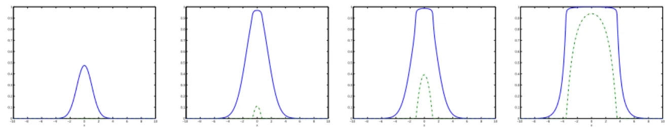
−100 −8 −6 −4 −2 0 2 4 6 8 10 0.1 0.2 0.3 0.4 0.5 0.6 0.7 0.8 0.9 1 x −100 −8 −6 −4 −2 0 2 4 6 8 10 0.1 0.2 0.3 0.4 0.5 0.6 0.7 0.8 0.9 1 x −100 −8 −6 −4 −2 0 2 4 6 8 10 0.1 0.2 0.3 0.4 0.5 0.6 0.7 0.8 0.9 1 x −100 −8 −6 −4 −2 0 2 4 6 8 10 0.1 0.2 0.3 0.4 0.5 0.6 0.7 0.8 0.9 1 x
Figure 1: First steps of the initiation of the free boundary. Results obtained thanks to a discretization of the system (2.1)–(2.2) with k = 100 and ν = 0.5. The density n is plotted in solid line whereas the pressure p is represented in dashed line. The pressure p has the same shape as in the classical Hele-Shaw system with growth. However the density n is smoother.
such that 0 ≤ n∞ ≤ 1, n∞(0) = nini, 0 ≤ p∞ ≤ PM, p∞ ∈ P∞(n∞), where P∞ is the Hele-Shaw
monotone graph given in (2.6). Moreover, the pair (n∞, p∞) satisfies on the one hand (2.5), and on
the other hand the Hele-Shaw type equation
∂tn∞− ∆p∞− ν∆n∞= n∞G¡p∞¢, (2.10)
and the complementarity relation (2.9) for almost every t > 0, all three equations in the weak sense. The time derivatives of the limit functions satisfy
∂tn∞, ∂tp∞∈ M1(QT), ∂tn∞, ∂tp∞≥ 0.
To illustrate this behaviour, we present numerical results obtained thanks to a discretization with finite volume of system (2.1)–(2.2) in the case k = 100, ν = 0.5 and with G(p) = 1 − p. We display
in Figure 1 the first steps of the formation of a tumor which is initially given by a small bump. As expected, we notice that the density n is smooth. The shape of the pressure p at the place where n = 1 is similar to the one observed for the classical Hele-Shaw system (see e.g. [17]).
The rest of the paper is organized as follows. We begin in Section 3 with some uniform (in k) a priori estimates which are necessary for strong compactness. Then, in Section 4 we prove the main statements in Theorem 2.1. The most delicate part, establishing (2.9), is postponed to Section 5. After proving uniqueness for the limit problem in Section 6, we end with a final section devoted to discuss further regularity issues and speed of the boundary of the tumor zone.
3
Estimates
To begin with, we gather in the following statement all the a priori estimates that we need later on.
Lemma 3.1 With the assumptions and notations in Theorem2.1, the weak solution (nk, pk) of (2.1)–
(2.2) satisfies 0 ≤ nk≤³ k − 1 k PM ´1/(k−1) −→ k→∞1, 0 ≤ pk≤ PM, Z Rd nk(t) ≤ eG(0)t Z Rd nini, Z Rd pk(t) ≤ CeG(0)t Z Rd nini.
with C a constant independent of k. Furthermore, there exists a uniform (with respect to k) nonnegative constant such that
Z Rd ³ ν|∇nk|2+ knk−1k |∇nk|2+ |∇pk|2 ´ (t) ≤ C³T, kninikL1(Rd)∩L∞(Rd) ´ for all t ∈ (0, T ). (3.1) Finally, ∂tnk, ∂tpk ≥ 0, ∂tnkis bounded in L∞((0, T ); L1(Rd)), ∂tpkis bounded in L1(QT).
Proof. Estimates on nk and pk. The L∞(Q) bounds are a consequence of standard comparison
arguments for (2.1) and (2.7). The L∞((0, T ); L1(Rd)) bound for nk can be obtained by integrating
(2.1) over Rdand then using (2.4). The L∞((0, T ); L1(Rd)) bound for p
know follows from the relation
between pk and nk.
Estimates on the time derivatives. We introduce the quantity
Σ(nk) = nkk+ νnk, Σ′(nk) = knk−1k + ν. (3.2)
The density equation (2.1) is rewritten in terms of this new variable as
∂tnk− ∆Σ(nk) = nkG(pk). (3.3)
Using the notation Σk = Σ(nk) and multiplying the above equation by Σ′(nk), we get
∂tΣk− Σ′k∆Σk= nkΣ′kG
¡
pk¢. (3.4)
Let wk= ∂tΣ(nk). Notice that sign (∂tnk) = sign (wk). A straightforward computation yields
∂twk− Σ′k∆wk = ∂tnkΣ′′k ¡ ∆Σk+ nkG(pk) ¢ + ∂tnkΣ′kG(pk) + ∂tnkΣ′kknk−1k G ′ (pk).
By using that wk= Σ′k∂tnkand Σ′(nk) = knk−1k +ν ≥ ν > 0, the right hand side of the above equation
can be written in a more handful way as ∂twk− Σ′k∆wk= wk ³Σ′′ k Σ′ k ¡ ∆Σk+ nkG(pk) ¢ + G(pk) + knk−1k G′(pk) ´ .
Since this equation preserves positivity and sign (wk(0)) = sign (∂tninik ) ≥ 0, we conclude that wk≥ 0,
that is, ∂tnk ≥ 0. The relation between pk and nk then immediately yields ∂tpk≥ 0.
Now that we know that the time derivatives have a sign, bounds for them follow easily. Indeed, using (2.1), we get k∂tnk(t)kL1(Rd) = d dt Z Rd nk(t) ≤ G(0)knk(t)kL1(Rd).
This gives the bound on ∂tnk in L∞([0, T ]; L1(Rd)). For ∂tpk we write
k∂tpkkL1(QT)= Z T 0 d dt µZ Rd pk(t) ¶ dt ≤ Z Rd pk(T ).
Estimates on the gradients. We multiply equation (2.1) by nk, integrate over Rdand use integration
by parts for the diffusion terms, Z Rd (nk∂tnk)(t) + Z Rd ¡ knk−1k |∇nk|2+ ν|∇nk|2¢(t) = Z Rd (n2kG(pk))(t) ≤ G(0) Z Rd n2k(t).
Since both nk and ∂tnk are nonnegative, we immediately obtain the estimate on the first two terms
in (3.1). On the other hand, integrating equation (2.7), we deduce Z Rd ∂tpk(t) + (k − 2) Z Rd ¡ |∇pk|2+ νknk−3k |∇nk|2 ¢ (t) = (k − 1) Z Rd (pkG(pk))(t) ≤ (k − 1)G(0) Z Rd pk(t).
Since ∂tpk≥ 0, we easily obtain the L2 bound on ∇pk in (3.1). ¤
4
Proof of Theorem
2.1
In this section we prove all the statements in Theorem2.1except the one concerning the complemen-tarity relation for the pressure, equation (2.9), whose proof is postponed to the next section.
Strong convergence and bounds. Since the families nkand pkare bounded in Wloc1,1(Q), we have strong
convergence in L1loc both for nkand pk. To pass from local convergence to convergence in L1(QT), we
need to prove that the mass in an initial strip t ∈ [0, 1/R] and in the tails |x| > R are uniformly (in k) small if R is large enough. The control on the initial strip is immediate using our uniform, in k and t, bounds for knk(t)kL1(Rd
) and kpk(t)kL1(Rd
). The tails for the densities nk are controlled using the
equation, pretty in the same way as it was done for the case ν = 0; see [17] for the details. The control on the tails of the pressures pkthen follows from the relation between pk and nk. Strong convergence
in Lp(QT) for 1 < p < ∞ is now a consequence of the uniform bounds for nk and pk.
Thanks to the a priori estimates proved above, we also have that (∇nk)k and (∇pk)k converge
weakly in L2(Q
T), and
0 ≤ n∞≤ 1, n∞, p∞∈ L∞((0, T ); H1(Rd)), ∂tn∞, ∂tp∞∈ M1(QT), ∂tn∞, ∂tp∞≥ 0.
Identification of the limit. To establish equation (2.5) in the distributional sense, we just pass to the limit, by weak-strong convergence, in equation (2.1) . On the other hand, using the definition of pk
in (2.2), we have nkpk= k k − 1n k k= ³ 1 −1k´1/(k−1)pk/(k−1)k −→ k→∞p∞.
Taking the limit k → ∞, we deduce the monotone graph property
p∞(1 − n∞) = 0. (4.1)
In order to show the equivalence of (2.10) and (2.5), we need to prove that ∇p∞= n∞∇p∞. This
es seen to be equivalent to p∞∇n∞= 0 by using the Leibnitz rule in H1(Rd) for (4.1). To prove the
latter identity, we first write pk∇nk= k k − 1n k k∇nk= √ k k − 1n (k+1)/2 k ¡√ k n(k−1)/2k ∇nk¢.
From estimate (3.1), the term between parentheses is uniformly bounded in L2(QT) and since (nk)k
is uniformly (in k) bounded in L∞(Q
T), we conclude that
lim
k→∞kpk∇nkkL2(QT)= 0.
We deduce then from the strong convergence of (pk)k and the weak convergence of (∇nk)k that
p∞∇n∞= 0, (4.2)
as desired.
Time continuity and initial trace. Time continuity for the limit density n∞ follows from the
mono-tonicity and the equation, as in the case ν = 0. Once we have continuity, the identification of the initial trace will follow from the equation for nk, letting first k → ∞ and then t → 0; see [17] for the
details.
Remark. Since p∞≥ 0, (4.2) implies that
∇p∞· ∇n∞= 0. (4.3)
5
The equation on p
∞In this section we give a rigorous derivation of equation (2.9), which is the most delicate point in the proof of Theorem 2.1.
(i) Our first goal is to establish that, in the weak sense,
p∞∆p∞+ p∞G(p∞) ≤ 0. (5.1)
Thanks to (4.2) and (4.3), this is equivalent to proving that p∞∆
¡
p∞+ νn∞
¢
+ p∞G(p∞) ≤ 0. (5.2)
In order to prove the latter inequality, we follow an idea of [17] and use a time regularization method `a la Steklov. To this aim, we introduce a regularizing kernel ωε(t) ≥ 0 with compact support of length ε.
Let nk,ε = nk∗ ωε. From equation (2.1), we deduce
∂tnk,ε− ∆ωε∗ (nkk+ νnk) = (nkG(pk)) ∗ ωε. (5.3)
Then, for fixed ε > 0, ∆ωε∗ (nkk+ νnk) is bounded in Lq(QT) for all q ≥ 1. Thus, we can extract
a subsequence such that (∇ωε∗ (nkk+ νnk))k converges strongly in L2(QT). Since we have strong
convergence of (nkk+ νnk)ktowards p∞+ νn∞, we deduce that the strong limit of (∇ωε∗ (nkk+ νnk))k
is equal to ∇ωε∗ (p∞+ νn∞).
Multiplying equation (5.3) by pk, we have
pk∂tnk,ε = pk∆¡nkk∗ ωε+ νnk,ε¢+ pk¡(nkG(pk)) ∗ ωε¢.
We can pass to the limit k → ∞ to get lim
k→∞pk∂tnk,ε = p∞∆
¡
To determine the sign, we decompose the left hand side term, divided by the harmless factor k/(k −1), as Z R nk−1k (t)∂tnk(s)ωε(t − s) ds = Z R nk−1k (s)∂tnk(s)ωε(t − s) ds | {z } Ak + Z R (nk−1k (t) − nk−1k (s))∂tnk(s)ωε(t − s) ds | {z } Bk .
On the one hand we have Ak= 1 k Z R ∂tnk(s)ωε(t − s) ds → 0 when k → ∞.
As for Bk, we recall that ∂tnk ≥ 0 provided ∂tnini ≥ 0; see Lemma 3.1. Thus, for s > t we have
nk−1k (t) − nk−1k (s) ≤ 0. Then, choosing ωε such that supp ωε ⊂ R−, we deduce that Bk ≤ 0, which
yields
p∞∆¡ωε∗ (p∞+ νn∞)¢+ p∞¡n∞G(p∞) ∗ ωε¢≤ 0.
It remains to pass to the limit ε → 0 in the regularization process. We can pass to the limit in the weak formulation since we already know that ∇p∞∈ L2(QT). Then, using (4.1), we get the inequality
(5.2) and thus (5.1).
(ii) Our second purpose is to establish the other inequality, namely
p∞∆p∞+ p∞G(p∞) ≥ 0. (5.4)
To prove it, we multiply equation (2.7) by a nonnegative test function φ(x, t) and integrate, and obtain Z Z QT φ¡pk∆pk+ pkG(pk) −νk−2k−1∇pkn·∇nk k ¢ = 1 k − 1 Z Z QT £ φ¡∂tpk− |∇pk|2¢+ ν∇φ · ∇pk¤.
From the proved bounds, the right hand side of the above equation converges to 0 as k → ∞. We can use integration by parts and rewrite the left hand side as
Z Z QT µ φpkG(pk) − pk∇φ · ∇pk− φ|∇pk|2− φνk(k − 2) k − 1 n k−3 k |∇nk|2 ¶ . Since the last term is nonpositive, we obtain that
lim inf k→∞ Z Z QT ¡ φpkG(pk) − pk∇φ · ∇pk− φ|∇pk|2 ¢ ≥ 0.
From weak-strong convergence in products, or convexity inequalities in the weak limit, we finally
conclude Z Z QT ¡ φp∞G(p∞) − p∞∇φ · ∇p∞− φ|∇p∞|2 ¢ ≥ 0. This is the weak formulation of (5.4).
Remark. A careful inspection of the proof of (5.4) shows that (2.8) holds if and only if ∇pk
converges strongly in L2(Q
T) and knk−3k |∇nk|2 converges weakly to 0 locally in L1(Q). Since we have
6
Uniqueness for the limit model
In this section we prove that the limit problem (2.10) admits at most one solution. We will adapt Hilbert’s duality method in the spirit of [17].
Theorem 6.1 Let T > 0, ν > 0. There is a unique pair (n, p) of functions in L∞([0, T ]; L1(Rd) ∩ L∞(Rd)), n ∈ C([0, T ]; L1(Rd)), n(0) = nini
, p ∈ P∞(n), satisfying (2.10) in the sense of distributions
and such that ∇n, ∇p ∈ L2(Q
T), ∂tn, ∂tp ∈ M1(QT).
Proof. Let us consider two solutions (n1, p1) and (n2, p2). Then for any test function φ with
φ ∈ W2,2(QT) and ∂tφ ∈ L2(QT), we have Z Z QT ³ (n1− n2)∂tφ + (p1− p2+ ν(n1− n2))∆φ +¡n1G(p1) − n2G(p2)¢φ ´ = 0, (6.1) which can be rewritten as
Z Z QT ¡ ν(n1− n2) + p1− p2¢¡A∂tφ + ∆φ + AG(p1)φ − Bφ¢= 0, (6.2) where 0 ≤ A = ν(n n1− n2 1− n2) + p1− p2 ≤ 1 ν, 0 ≤ B = −n2 G(p1) − G(p2) ν(n1− n2) + p1− p2 ≤ κ,
for some nonnegative constant κ. To arrive to these bounds on A we set A = 0 when n1= n2, even if
p1 = p2. Since A can vanish, we use a smoothing argument by introducing the regularizing sequences
(An)n, (Bn)nand (G1,n)n such that
kA − AnkL2(QT) < α/n, 1/n < An≤ 1,
kB − BnkL2(QT) < β/n, 0 ≤ Bn≤ β2, k∂tBnkL1(QT)≤ β3,
kG1,n− G(p1)kL2(QT) ≤ δ/n, |G1,n| < δ2, k∇G1,nkL2(QT) ≤ δ3,
for some nonnegative constants α, β, β2, β3, δ, δ2, δ3.
Given any arbitrary smooth function ψ compactly supported, we consider the solution φn of the
backward heat equation ∂tφn+ 1 An ∆φn+ G1,nφn− Bn An φn= ψ in QT, φn(T ) = 0. (6.3)
The coefficient 1/An is continuous, positive and bounded below away from zero. Then the equation
satisfied by φn is parabolic. Hence φn is smooth and since ψ is compactly supported, we have that
φn, ∆φn and therefore ∂tφn are L2-integrable. Therefore, we can use φn as a test function in (6.2).
Then, by the definition of A, we have Z Z QT (n1− n2)ψ = Z Z QT ¡ ν(n1− n2) + p1− p2¢Aψ.
Inserting (6.3) and substracting (6.2), we obtain Z Z QT (n1− n2)ψ = I1n+ I2n+ I3n, where I1n= Z Z QT ¡ ν(n1− n2) + p1− p2¢³¡ A An − 1 ¢¡ ∆φn− Cnφn¢´, I2n= Z Z QT ¡ ν(n1− n2) + p1− p2¢(B − Bn)φn, I3n= Z Z QT (n1− n2)¡G1,n− G(p1)¢φn.
The convergence towards 0 of the terms Iin, i = 1, 2, 3 is now a consequence on some estimates
on the test functions φn which are gathered in Lemma 6.2 below. Indeed, applying the mentioned
estimates and Cauchy-Schwarz inequality we have I1n≤ Kk(A − An)/√AnkL2(QT)≤ K √ nkA − AnkL2(QT)≤ Kα/ √n, I2n≤ KkB − BnkL2(QT)≤ Kγ/n, I3n≤ Kδ/n,
(in all the computations, K denotes various nonnegative constants). Then letting n → ∞, we conclude
that Z Z
QT
(n1− n2)ψ = 0,
for any smooth function ψ compactly supported, hence n1 = n2. It is then obvious, thanks to (6.1),
that p1= p2. ¤
Lemma 6.2 Under the assumptions of Theorem6.1, we have the uniform bounds, only depending on T and ψ, kφnkL∞(Q T)≤ κ1, sup 0≤t≤Tk∇φn(t)kL 2(Rd )≤ κ2, k1/ p An(∆φn− Bnφn)kL2(QT)≤ κ3.
Proof. The first bound is a consequence of the maximum principle on (6.3). Then multiplying (6.3) by ∆φn− Bnφn and integrating on Rd, we get
−12dtd Z Rd|∇φn(t)| 2 −12dtd Z Rd Bnφ2n(t) + Z Rd 1 An|∆φn− Bn φn|2(t) + 1 2 Z Rd (∂tBnφ2n)(t), = Z Rd ³ G1,n|∇φn|2+ φn∇φn· ∇G1,n+ BnG1,nφ2n+ (∆ψ − Bnψ)φn ´ (t). After an integration in time on [t, T ], we deduce
1 2k∇φn(t)kL2(Rd)+ Z T t Z Rd 1 An|∆φn− Bn φn|2 ≤ K ³ 1 − t + Z T t k∇φn(s)kL 2(Rd )ds ´ ,
where we use the bounds on ∇G1,n and ∂tBn by construction of the regularization. We conclude by
7
Further regularity and velocity of the free boundary
Remember that both p∞and n∞belong to H1(Rd) for almost every t > 0. This regularity cannot be
improved, because there are jumps in the gradients of both p∞ and n∞ at the free boundary. As a
consequence, their laplacians are not functions, but measures. However, these singularities cancel in the combination Σ∞= p∞+ νn∞, as we will see now.
Lemma 7.1 With the assumptions of Theorem 2.1, the quantity Σ∞ belongs to L2((0, T ); H2(Rd))
for all T > 0 and we have the estimate Z Z
QT
(∆Σ∞)2≤ C(T ).
Proof. We recall the definition of Σk in (3.2). Since ∇Σk = nk∇pk+ ν∇nk, estimate (3.1) yields
that for all 0 < t ≤ T , Z
Rd|∇Σk(t)|
2
≤ C(T ).
We now multiply the equation (3.4) by ∆Σk, and integrate in QT, 0 < T < ∞, to obtain, using that
Σ′k> ν and the fact that both nk and G(pk) are nonnegative,
Z Z QT (∆Σk)2 ≤ 1 2 Z Rd|∇Σk| 2(0) + C(T ).
The result follows directly. ¤
This implies in particular that in the limit Σ∞(·, t) ∈ H2(Rd) for almost every t > 0. Hence, the size
of the jump (downwards) of ∇p∞ at the free boundary coincides with the size of the jump (upwards)
of ν∇n∞ there.
Concerning the time regularity, the limit equation for the density (3.3), now tells us that ∂tn∞ ∈
L2(QT). Hence n∞ ∈ H1(QT). We do not have a similar property for the pressure (think of the
situation when two tumors meet).
Our last goal is to derive formally an asymptotic value for the free boundary speed in a particular example. Let Ω(t) denote, as before, the space filled by the tumor at time t. We notice that n∞solves
∂tn∞= ν∆n∞+ G(0)n∞, x ∈ Rd\ Ω(t), t > 0,
with boundary conditions
n∞= 1, ν∂nn∞= ∂np∞, x ∈ ∂Ω(t), t > 0.
If Ω(t) were known, the problem would be overdetermined. This is precisely what fixes the dynamics of the free boundary. Let us assume that the tumor is a ball centered at the origin,
Ω(t) = {x : p∞(x, t) > 0} = {x : n∞(x, t) = 1} = BR(t)(0).
We look for a solution which is spherically symmetric n∞(r, t), p∞(r, t). We set σ = R′(t). In
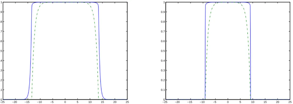
−250 −20 −15 −10 −5 0 5 10 15 20 25 0.1 0.2 0.3 0.4 0.5 0.6 0.7 0.8 0.9 1 x −250 −20 −15 −10 −5 0 5 10 15 20 25 0.1 0.2 0.3 0.4 0.5 0.6 0.7 0.8 0.9 1 x
Figure 2: Shape of the traveling waves obtained thanks to a numerical discretization of the system (2.1)–(2.2) with k = 100 and ν = 0.5 (left) or ν = 0 (right) for the same initial data and the same final time. The density n is plotted in line whereas the pressure is represented in dashed line. We notice the regularity of n in the case ν = 0.5, whereas it has a jump at the interface when ν = 0. Also the free boundary moves faster when active motion is present.
with constant speed. However, following [17] Appendix A, we expect our solution to behave for large times as a one dimensional traveling wave (with constant speed).
In order to analyze the expected asymptotic constant speed, we set nR(r − σt) = n∞(r, t) and
pR(r − σt) = p∞(r, t). Introducing this ansatz in equation (2.10), we obtain
− σn′R= p′′R+d − 1r p′R+ νn′′R+ νd − 1r n′R+ nRG(pR). (7.1)
On Rd\ Ω(t), we have p∞= 0, then integrating (7.1) in (R(0), ∞), we get
σnR(R(0)) = −νn′R(R(0)+) + ν(d − 1) Z ∞ R(0) n′ R r dr + G(0) Z ∞ R(0) nRdr.
In a one dimensional setting (d = 1) and using the boundary relation at the interface of Ω(0), we deduce
σ = −p′R(R(0)−) + G(0)
Z ∞ R(0)
nR(r)dr. (7.2)
We recall that for the classical Hele-Shaw model without active motion (i.e. ν = 0), the traveling velocity is σ0 = −p′R(R(0)−). Since nR(R(0)) = 1 and nR is continuous and nonnegative, we have
R∞
R(0)nR(r)dr > 0. Then we conclude from equation (7.2) that σ > σ0.
We can do a more precise computation confirming the above statement for the one-dimensional case. From the complementarity relation (2.9), we have −p′′
R= G(pR) on Ω(0). Multiplying this latter
equation by p′
R and integrating on (0, R(0)), we deduce
p′R(R(0)−)2 = 2 Z R(0)
0
In the center of the tumor, we expect a maximal packing of the cells. Therefore, we have the boundary conditions lim r→0pR(r) = PM, r→0limp ′ R(r) = 0. Since p′′
R= −G(pR) ≤ 0, we deduce that p′R< 0 and we can make the change of variable
p′R(R(0)−)2 = 2 Z R(0) 0 p′RG(pR) dr = 2 Z PM 0 G(q) dq. The quantity σ0 = q 2RPM
0 G(q) dq is the traveling velocity for a tumor spheroid in the case ν = 0;
see Appendix A.1 of [17]. Combining this with (7.2), we deduce that the growth of the tumor is faster with active motion than in the case ν = 0.
In Figure 2, we display numerical simulations obtained from a discretization with a finite volume scheme of system (2.1)–(2.2) for k = 100. The left picture presents the result for ν = 0.5, and the right for ν = 0 (i.e. without active motion). We use the growth function G(p) = 1 − p and the results in both cases with the same initial data and at final time t = 10. We notice that in the case ν = 0.5 the density function is smooth and the domain occupied by the tumor is larger than in the case without active motion, which suggests as explained above a faster invasion speed.
References
[1] Bellomo, N.; Li, N. K.; Maini, P. K. On the foundations of cancer modelling: selected topics, speculations, and perspectives. Math. Models Methods Appl. Sci. 18 (2008), no. 4, 593–646.
[2] B´enilan, Ph.; Igbida, N. La limite de la solution de ut= ∆pum lorsque m → ∞. C. R. Acad. Sci.
Paris S´er. I Math. 321 (1995), no. 10, 1323–1328.
[3] Betteridge, R.; Owen, M. R.; Byrne, H. M.; Alarc´on, T.; Maini, P. K. The impact of cell crowding and active cell movement on vascular tumour growth. Netw. Heterog. Media 1 (2006), no. 4, 515–535.
[4] Br´u, A.; Albertos, S.; Subiza, J. L.; Asenjo, J. A.; Brœ, I. The universal dynamics of tumor growth. Biophys. J. 85 (2003), no. 5, 2948–2961.
[5] Byrne, H. M.; Chaplain, M. A. Growth of necrotic tumors in the presence and absence of in-hibitors. Math. Biosci. 135 (1996), no. 15, 187–216.
[6] Byrne, H. M.; Drasdo, D. Individual-based and continuum models of growing cell populations: a comparison. J. Math. Biol. 58 (2009), no. 4-5, 657–687.
[7] Byrne, H. M.; Preziosi, L. Modelling solid tumour growth using the theory of mixtures. Math. Med. Biol. 20 (2003), no. 4, 341–366.
[8] Chaplain, M. A. J. Avascular growth, angiogenesis and vascular growth in solid tumours: the mathematical modeling of the stages of tumor development. Math. Comput. Modeling 23 (1996), no. 6, 47–87.
[9] Ciarletta, P.; Foret, L.; Ben Amar, M. The radial growth phase of malignant melanoma: multi-phase modelling, numerical simulations and linear stability analysis. J. R. Soc. Interface 8 (2011) no. 56, 345–368.
[10] Cui, S. Formation of necrotic cores in the growth of tumors: analytic results. Acta Math. Sci. Ser. B Engl. Ed. (2006), no. 4, 781–796.
[11] Cui, S.; Escher, J. Asymptotic behaviour of solutions of a multidimensional moving boundary problem modeling tumor growth. Comm. Partial Differential Equations 33 (2008), no. 4–6, 636– 655.
[12] Drasdo, D.; Hoehme, S. Modeling the impact of granular embedding media, and pulling versus pushing cells on growing cell clones. New J. Phys. 14 (2012) 055025 (37pp).
[13] Friedman, A.; Hu, B. Stability and instability of Liapunov-Schmidt and Hopf bifurcation for a free boundary problem arising in a tumor model. Trans. Am. Math. Soc. 360 (2008), no. 10, 5291–5342.
[14] Gil, O.; Quir´os, F. Boundary layer formation in the transition from the porous media equation to a Hele-Shaw flow. Ann. Inst. H. Poincar´e Anal. Non Lin´eaire 20 (2003), no. 1, 13–36.
[15] Greenspan, H. P. Models for the growth of a solid tumor by diffusion. Stud. Appl. Math. 51 (1972), no. 4, 317–340.
[16] Lowengrub, J. S.; Frieboes H. B.; Jin, F.; Chuang, Y.-L.; Li, X.; Macklin, P.; Wise, S. M.; Cristini, V. Nonlinear modelling of cancer: bridging the gap between cells and tumours. Nonlinearity 23 (2010), no. 1, R1–R91.
[17] Perthame, B.; Quir´os, F.; V´azquez, J. L. The Hele-Shaw asymptotics for mechanical models of tumor growth. Arch. Ration. Mech. Anal., to appear.
[18] Preziosi, L.; Tosin, A. Multiphase modelling of tumour growth and extracellular matrix interaction: mathematical tools and applications. J. Math. Biol. 58 (2009), no. 4-5, 625–656.
[19] Ranft, J.; Basana, M.; Elgeti, J.; Joanny, J.-F.; Prost, J.; J¨ulicher, F. Fluidization of tissues by cell division and apoptosis. Proc. Natl. Acad. Sci. USA (2010), no. 49, 20863–20868.
[20] Roose, T.; Chapman, S. J.; Maini, P. K. Mathematical models of avascular tumor growth. SIAM Rev. 49 (2007), no. 2, 179–208.
[21] Saut, O.; Lagaert, J.-B.; Colin, T.; Fathallah-Shaykh, H. M. A multilayer grow-or-go model for GBM: effects of invasive cells and anti-angiogenesis on growth. Preprint 2012.
[22] Tang, M.; Vauchelet, N.; Cheddadi, I.; Vignon-Clementel, I.; Drasdo, D.; Perthame, B. Composite waves for a cell population system modelling tumor growth and invasion. Chin. Ann. Math. Ser. B 34 (2013), no. 2, 295–318.
[23] V´azquez, J. L. “The porous medium equation. Mathematical theory”. Oxford Mathematical Monographs. The Clarendon Press, Oxford University Press, Oxford, 2007. ISBN: 978-0-19-856903-9.