A comparative study of several dynamic time warping algorithms for speech recognition

TIME WARPING ALGORITHMS FOR SPEECH RECOGNITION

by

Cory S. Myers

SUBMITTED IN PARTIAL FULFILLMENT OF THE REQUIREMENTS FOR THE DEGREES OF

BACHELOR OF SCIENCE and

MASTER OF SCIENCE at the

MASSACHUSETTS INSTITUTE OF TECHNOLOGY February 1980

' BELL TELEPHONE LABORATORIES, INCORPORATED Signature of Author ...

/Department of Electrical Engineering and (I,

...

-7h

Thesis Supervisor ...Acadeic) Thesis Supervisor (Academic)

Certified

by...

...

Company Survisor (VI-A Cooperating Company)

certified by...

.

empa.y

.

Sug

r (V tCooperating Company)

Accepted by. _._

-' hairman, Departmental Committee on Graduate Students

ARCHIVES MASSACHUSETTS INSTITUTE

OF TECHNOLOGY

JUN 2

0 1980

A COMPARATIVE STUDY OF SEVERAL DYNAMIC TIME WARPING ALGORITHMS FOR SPEECH

RECOGNITION

by

Cory S. Myers

Submitted to the Department of Electrical Engineering and Computer Science on February 4, 1980, in partial fulfillment of the requirements for the Degrees of Bachelor of Science and Mas-ter of Science.

ABSTRACT

A comparative study of several dynamic time warping algorithms for speech recognition was conducted, Performance measurements based on memory usage, recognition accuracy and computational speed were made. The first part of the investigation involved dynamic time warping for isolated word recognition. It was assumed that the word endpoints had been reli-ably obtained. Factors which were considered included local continuity constraints on the dynamic path, global range constraints and the type of normalization. Broad classifications were made to highlight the strengths and weaknesses of the various algorithms. In addition, a new approach to dynamic time warping for isolated word recognition was examined. This approach applied linear normalization to both the test and the reference utterance prior to a non-linear time warping. Results of experiments on this algorithm show comparable performance to the other dynamic time warping algorithms investigated. The practical importance of this new method is presented in the thesis,

In the second part of the investigation two general dynamic time warping algorithms for word spotting and connected speech recognition are described. These algorithms are called the fixed range and the local minimum method. The characteristics and properties of these algo-rithms are discussed. It is shown that the local minimum method performs considerably better than the fixed range method. Explanations of this behavior are given and an optimized method of applying the local minimum algorithm is discussed. It is shown that, for word spotting prob-lems, successive trials of the local minimum algorithm need not be made at every possible starting point in order to achieve good accuracy. We also demonstrate that one reasonable approach to connected speech recognition is to build reference strings using a single local minimum time warp per word of the test utterance and hypothesizing the beginning of one word based on the end of the previous word.

THESIS SUPERVISOR: Jae S. Lim

TITLE: Assistant Professor of Electrical Engineering and Computer Science THESIS SUPERVISOR: Aaron E. Rosenberg

TITLE: Member of Technical Staff at Bell Telephone Laboratories THESIS SUPERVISOR: Lawrence R. Rabiner

ACKNOWLEDGEMENTS

I wish to express my sincere gratitude to my two advisors at Bell Laboratories, Dr. Aaron E. Rosenberg and Dr. Lawrence R. Rabiner, for their guidance, encouragement and helpful suggestions. Further special thanks is due to Dr. Rabiner for his continued enthusiasm and his suggestions regarding the writing of this manuscript. I am also particularly indebted to Dr. James L. Flanagan of Bell Laboratories for inviting me to work in his department and for pro-viding all the necessary facilities, and to Dr. Jae S. Lim of MIT for agreeing to be my thesis supervisor.

I wish also to thank Mrs. Kathy L. Shipley for her assistance in the learning of the use of the computer system and for her help in the software development. Special thanks is also due both the Word Processing and the Drafting Departments of Bell Laboratories for their fine work.

Additional thanks is due to Jay Wilpon for his help in providing data files and for his encouragement and to Lori Lamel for her encouragement and helpful comments on the writing of this thesis.

Finally, I am sincerely thankful to my parents, Perry and Eleanor Myers, for their continu-ing love, support and encouragement.

TABLE OF CONTENTS

TITLE PAGE... I

ABSTRACT

...

2

ACKNOW LEDGEM ENTS ... ... 3

TABLE OF CONTENTS ... 4

LIST OF FIGURES AND TABLES ... 7

TABLE OF SYM BOLS ... 10

CHAPTER 1 INTRODUCTION ... 13

1.1 Speech Recognition Systems ... 13

1.2 Time W arping ... 15

1.3 The W ork Undertaken in This Thesis ... 16

1.4 Organization of Subsequent Chapters ... 18

CHAPTER 2 FUNDAMENTALS OF DYNAMIC TIME WARPING ... 20

2.1 General Description of the Problem ... 20

2.2 Time W arping as Path Finding ... 25

2.2.1 Endpoint Constraints ... 25

2.2.2 Local Continuity Constraints ... 26

2.2.3 Global Path Constraints ... 32

2.2.4 Axis Orientation ... 36

2.2.5 Distance M easures ... 36

2.2.6 Solution for the Optimal Path ... 46

2.3 Dynamic Time W arping ... 46

2.4 Summary ... 62

CHAPTER 3 PERFORMANCE MEASURES FOR DYNAMIC TIM E W ARPING ALGORITHM S ... 63...

3.1 Introduction ... 63

3.1.1 The Isolated W ord Recognizer ... 63

3.2.1 M emory Requirem ents ... 70

3.2.2 Computational Efficiency (Speed of Execution) ... 71

3.2.3 Recognition Accuracy ... 72

3.3 Sum m ary ... 75

CHAPTER 4 RESULTS ON ISOLATED WORD RECOGNITION ... ... 76

4.1 Initial Experiments ... 76

4.2 Experim ental Results ... 78

4.2.1 Memory Requirements ... 79

4.2.2 Com putational Efficiency ... 79

4.2.3 Recognition Accuracy ... 89

4.3 D iscussion ... 97

4.4 Normalize/Warp Algorithm ... 99

CHAPTER 5 SUMMARY OF RESULTS FOR ISOLATED WORD RECOGNITION ... 105

5.1 Introduction ... 105

5.1.1 M em ory Requirem ents ... 105

5.1.2 Com putational Efficiency ... 105

5.1.3 Recognition Accuracy ... 106

5.1.4 T radeo ffs ... ... ... 106

5.2 Results Concerning the Normalize/Warp Algorithm ... 107

5.3 Practical Significance ... 107

5.4 Future Research A reas .. ... 108

CHAPTER 6 ISSUES IN DYNAMIC TIME WARPING FOR CONNECTED SPEECH RECOGNITION ... 109

6.1 Introduction ... 109

6.1.1 Basic Difficulties in Connected Speech Recognition Using Word S ize T em plates ... ... 1 10 6.1.2 Basic Approaches to the Problems of Connected Speech Recognition ... 112

6.3 Issues in the Dynamic Time Warping Algorithms ... 120

CHAPTER 7 EXPERIMENTS IN DYNAMIC TIME WARPING FOR CONNECTED SPEECH RECOGNITION ... 123

7.1 Introduction ... ...123

7.2 Comparison of the Two Time Warping Algorithms ... 123

7.3 Examination of the Parameters of the Local Minimum Dynamic Time Warping Algorithm ... 125

CHAPTER 8 SUMMARY OF RESULTS ON DYNAMIC TIME WARPING FOR CONNECTED SPEECH RECOGNITION ... ... 134

8.1 Introduction ... 134

8.1.1 Relative Performance of the Fixed Range and the Local Minimum Time Warping Algorithms ... 134

8.1.2 Optimal Choice of the Parameters of the Local Minimum time Warping Algorithm ... 134

8.2 Practical Significance of the Results ... 135

8.3 Future Research Areas ... ... 135

REFERENCES ... ... .. ... 137

APPENDIX I TIME WARPING FOR CONTINUOUS FUNCTIONS ... 140

LIST OF FIGURES AND TABLES

FIGURES

Figure Page

1.1 - Block Diagram of an Automatic Speech

Recognition System ... 14

1.2 - Example of Time Warping ... ... 17

2.1 - T im e W arping ... 21

2.2 - Discrete - Time Time Warping ... 23

2.3 - Time Warping as Path Finding ... 24

2.4 - Type I Local Constraints ... 27

2.5 - Sample Path ... 30

2.6 - Local Constraints Types 11 and III ... 31

2.7 - Global Range for Paths ... 34

2.8 - Global Range for Paths as a Function of N/M ... 35

2.9 - Global Range for Paths with Range Limiting ... 37

2.10 - Weighting Functions for Type II Paths ... 40

2.11 - Weighting Functions for Type I Paths ... 41

2.12 - Sample Path with Distance Measure ... 42

2.13 - Tw o D ifferent Paths ... 44

2.14 - Sample Accumulated Distance Functions ... 54

2.15 - Typical Dynamic Time Warping Results ... 55

2.16 - Type IV Local Constraints ... 60

2.17 - Itakura's Dynamic Time Warping Algorithm ... 61

3.1 - Isolated Word Recognition System ... 64

3.2 - Probability Distributions for Distance Scores ... 74

4.1 - Plot of Computational Time Versus Range Limit ... ... 84

4.3 - Warps Performed Plotted as a Function

of Range Limit ... 88

4.4 - Error Rate as a Function of Local Constraints and Axis Orientation ... 90

4.5 - Distance Scores for Local Constraints Types Ill and IV . ... ... 91

4.6 - Distance Scores for Reference Along X-Axis and Test Along X-Axis ... 94

4.7 - Error Rate Plotted as a Function of Range Limit and Distance as a Function of N/M ... 98

4.8 - Log Magnitude of the Transform of a Typical Reference Pattern Component ... ... 100

4.9 - Error Rate of the Normalize/Warp Algorithm ... 102

4.10 - Normalize/Warp Results as a Function of Range Limit ... ... ... 1... 104

6.1 - Log Energy for Two Speech Utterances ... ... 11... 111

6.2 - Illustration of the General Time Warping Problem ... 113

6.3 - Expanded Range for a Single Time Warp ... 117

6.4 - Illustration of the Fixed Range and the Local Minimum DTW Algorithms ... 1... 119

6.5 - Illustration of the Parameters in the Local Minimum DTW Algorithm ... 121

7.1 - Results for Word Recognition Using Both the Fixed Range and the Local Minimum DTW Algorithms ... 124

7.2 - Results for Word Spotting Using Both the Fixed Range and the Local Minimum DTW Algorithms ... 126

7.3 - Distance Scores for the Local Minimum DTW Algorithm as Applied to Connected Word Recognition ... 128

7.4 - Illustration of Path Merging for Two Adjacent Local Minimum Time Warps ... ... 130

7.5 - Digit Error Rate for Connected Digit Recognition Using Local Minimum DTW Algorithm and Several Values of E and 8 ... 131

7.6 - Digit Error Rate for Connected Digit Recognition Using the Local Minimum DTW Algorithm ... 133

TABLES

Table Page

2.1 - L ocal C on straints ... ... 47

2.2 - Endpoint and G lobal Constraints ... 48

2.3 - Axis Orientation and Distance Measures ... 49

2.4 - Weighting Functions ... 0

2.5 - Accumulated Distance Functions ... 57

4.1 - 54 W ord V ocabulary ... ... 77

4.2 - Memory Requirements ... 80

4.3 - Combinatorics Time by Local Constraints ... 82

4.4 - Combinatorics Time by Weighting Function ... 83

4.5 - Local D istance Calculation s ... ... 87

4.6 - Error Rates by Weighting Function ... ... 96

A2.1 - Tim ing Results - Average Per W arp ... 146

A2.2 - Range Size (N=40)) ... 147

A 2.3 - W arps Perl'orm e d ... ... 149

A2.4 - Recognition Accuracy ... 150

A2.5 - Distance Between Same Words ... 151

Table of Symbols

a,b

aj

c(k)

d(i(k),j(k))

d(t,w(t))

d(R(n),T(m))

d((n',m'),(n,m))

D (i(k),j(k))

D(w(t))

b

D( ''(i(k),j(k))

E

F(t, w(t),

O(t))

g(k)

H(z)

(i(k),j (k))

K'

M

initial and final values of t for the general calculus of variations problem j it linear prediction coefficient

j"' linear prediction coefficient for the n "' frame of the reference bounds on the beginning region in a test pattern

middle of a beginning region size of a beginning region

local minimum of DA (i(k)-l,j) along the j axis

distance between frame i(k) of the reference and j(k) of the test distance between location t of the reference and w(t) of the test distance between frame n of the reference and frame m of the test a constant distance value

distance from a point (n',m') to a point (n, m) via the best possible path normalized distance along a path defined by the functions i(k) and j(k) normalized distance along a curve defined by the function w (t)

best normalized distance along any path

normalized distance along path defined by i(k) and j(k) and using refer-ence pattern v

best normalized distance along path using reference pattern v accumulated distance to the point (n,m) along the best path to it bounds on the ending region in a test pattern

size of an ending region il' order LPC residual energy maximum allowable slope of a path minimum allowable slope of a oath a function of t, w(t) and i (t)

Itakura's dynamic time warping function designed to limit compression of a reference pattern

transfer function of a system parameterized path functions length of path

length of a subsection of a path length of the r ' production

bounds on the position of speech in a test pattern length of the speech component of a test pattern normalized length of the test pattern

bounds on the position of speech in a reference pattern length of the speech component of a reference pattern normalized length of the reference pattern

normalization factor associated with weighting function W samples used per frame

number of local minimum time warps order of an LPC production

probability density function of distances for reference and test different probability density function of distance for reference and test the same

rt h _{production rule}

probability of a false alarm probability of a miss

cumulative probability distribution of pD(D) cumulative probability distribution of ps(D) range limit, in frames

a reference pattern, both discrete and continuous time ith component of R(n)

normalized length reference pattern

I"h autocorrelation

Ith autocorrelation of the m'1h frame of the test speech signal

filtered speech signal sampling period for frames

a test pattern, both discrete and continuous time i'hcomponent of T(m)

normalized length test pattern

index of the reference pattern which best matches a test pattern vocabulary size

initial and final values for the general calculus of variations problem a warping function, both discrete and continuous time

a windowing function

discrete time path weighting function continuous time curve weighting function samples of S(n) within a frame

windowed samples of x(n)

jth order LPC coefficient after i iterations of Durlin's recursion

Ith element of the rth production rule

Ni,N2

N

N(W)

Pt,

PD(D)

Ps(D)

R(n),R(t)

R(n,i)

S(n)

(l)

s(n)

S(n)

T(m),T(r)

T(m,i)

w(n),w(t)

W(n)

W (t,w(t),

W(t) )

x(n)

x(n)

8 separation between beginning regions for several local minimum time warps

A total range covered by several local minimum time warps E local range in the local minimum time warp

(D threshold for overlapping probability distributions

(t) a function of t

(t) derivative of +(t) with respect to t partial derivative of , with respect to x

Chapter 1

Introduction

1.1 Speech Recognition Systems

An important step in the realization of man-machine communications is the development of a practical speech recognition system. Work over the past decades has advanced automatic speech recognition systems to the point where such systems are being used (in some cases on an experimental basis) for such diverse applications as directory assistance [1] and voice control of machinery on an assembly line [21. However, such applications are still severely limited with regard to vocabulary size, type of speech input, and the environment under which these recog-nizers can properly function. These constraints arise from the inherent complexity of the speech recognition problem along with the massive amounts of computation generally required to "solve the broad speech recognition problem."

Several factors determine the performance of speech recognition systems. A system may be able to handle a large vocabulary or a small one. The input speech utterances may be as simple as single, isolated letters, digits or words, or as complex as complete sentences. Speech recog-nition systems are also classified as being either speaker independent or speaker dependent. Speaker dependent systems require a learning period in which the machine is trained to the

user's voice. Speaker independent systems, while more versatile in their ability to handle a wide class of talkers without individualized training, are generally more complex and costly.

Many speech recognition systems rely on pattern matching concepts. Such systems have many basic features in common, the major components of which are depicted in the block diagram of Figure 1.1. First the input utterance is filtered, digitized, and analyzed to determine the beginning and ending points of the speech (i.e. to separate the spoken text from the back-ground silence). Next, a set of features is measured for the speech in order to represent the utterance in a form more amenable to recognition (i.e. in a data reduced format). Common parametrizations include some or all of the following measurements: zero crossing rates, linear

u

Z (J

r.

predictive coding (LPC) coefficients, spectral coefficients, cepstral coefficients, etc. In a typical recognition system, these parameters are calculated once every frame, where a frame is typically 20 to 50 milliseconds in duration. Usually, a new frame is calculated every 10 to 30 mil-liseconds (i.e. frames generally overlap in time). The resulting time sequence of features for the test utterance is defined to be a test pattern. In order to determine what speech is present in the test utterance, the parametrized speech is compared to a set of stored reference patterns consisting of previously parametrized words, syllables or phonemes (obtained from a training

set of data), and the "best" fit is selected as the most likely candidate for the speech utterance. For purposes of our investigations into word recognition the unit of recognition will be isolated words. As we shall see in Chapter 2, such an assumption will be fundamental, in that, the use of a smaller recognition unit will require either accurate segmentation of the input utterance or the use of an entirely different time warping procedure than the one which will be used.

In order to obtain such a "best fit", we are faced with the problem of comparing a test tern with a set of reference patterns. Generally, the time scales of the test and reference pat-terns are incommensurate. However, even if the time scales are the same, it is highly unlikely that the timing of the test precisely matches the timing of each reference. As such, we must use some method of time warping to optimally register the test pattern with each reference pat-tern. We discuss the problem of time warping in the next section.

1.2 Time Warping

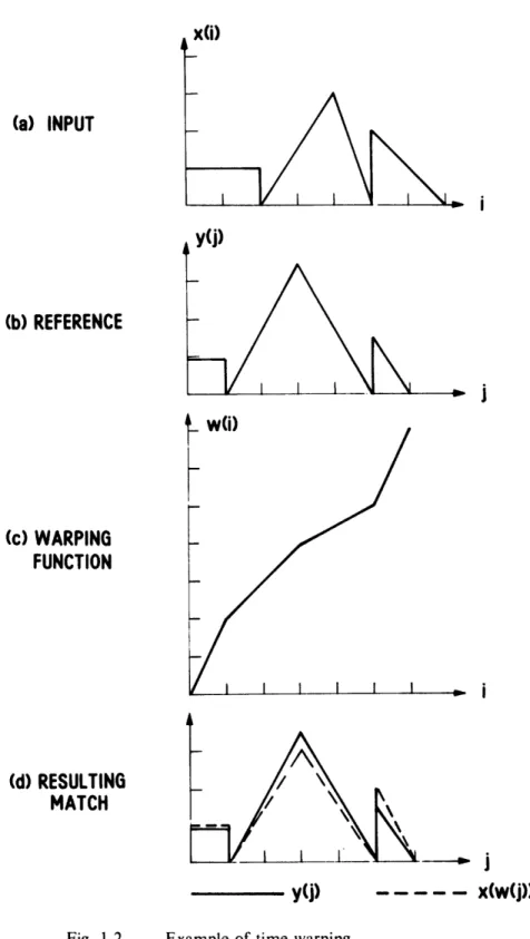
In order to properly compare the parametrized representation of an input speech signal (the test pattern) with a reference pattern, temporal variations between the two patterns, due to differences in the way in which a speaker may say the same utterance at two different occasions, must be compensated for. Such temporal variations can include absolute differences in the length of a test pattern and its corresponding reference pattern, as well as local variations in which the test utterance may be sped up at one section of time and slowed down at another relative to the reference pattern. Time alignment, or time warping, is a procedure in which the input utterance's temporal feature set is locally stretched and/or compressed in order to achieve

the best possible match to the reference. Figure 1.2 shows an example of time warping one function to fit another. art a shows the input signal and part b shows the reference to which the input is to be matched. The time warping function is shown in part c and the resulting match between the input and the reference is shown in part d. It is clear from this simple example that time warping can provide significant improvements in matching two patterns.

The simplest implementation of time warping is linear compression or expansion of the input utterance to the reference. While this method is often satisfactory for monosyllabic words [3], it is generally unsatisfactory for polysyllabic words or sentences. In 1971, Sakoe and Chiba proposed the use of dynamic time warping to improve the fit between reference and test patterns [4]. In this method, a nonlinear expansion and/or compression of the time scale is used to provide an optimal fit between the patterns. Sakoe and Chiba also suggested the use of dynamic programming, as developed by Bellman [5] in 1962, for the efficient implementation of the time warping algorithm. Such implementations of the time warping algorithm have sub-sequently led to great improvements in speech recognition systems [4,6,71. The basic com-ponents of a dynamic time warping (DTW) algorithm include a distance metric (for comparing frames of the test and reference), the specification of local and global continuity constraints (to determine the warping contour), and endpoint constraints (to define initial and final registration of the test and reference). The DTW distance measure appropriate for speech recognition is dependent on the feature set used for parametrization. For example, a log spectral difference is suitable for bandpass filter parameters, a Euclidean distance is suitable for cepstral coefficients, and a log likelihood ratio, as originally proposed by Itakura [6], is suitable for LPC coefficients. Global and local continuity constraints are used to insure that time continuity is preserved in the warped pattern, and that excessive warping is not used in the procedure - e.g. locally or glo-bally expanding a very short utterance to match a very long one.

1.3 The Work Undertaken in this Thesis

In the work undertaken in this thesis, several previously proposed and some new dynamic time warping algorithms are compared. For each of the algorithms, measurements of

computa-(a) INPUT (b) REFERENCE (c) WARPING FUNCTION (d) RESULTING MATCH vfil w(i) i

Fig. 1.2 Example of time warping.

y(j)

---

x(w(j))

tional efficiency, recognition accuracy and memory requirements are made. To perform these measurements, a feature set based on an eighth order LPC analysis for each speech frame was

used. As such, the log likelihood ratio distance measure of Itakura was used as the distance metric. A standard set of speakers and reference templates, corresponding to a set of isolated words, was used to test all the DTW algorithms. Two major application areas of the DTW algo-rithms are examined in this thesis; namely, dynamic time warping for isolated word recognition, and dynamic time warping for continuous speech recognition. Tradeoffs among memory usage, computational efficiency and recognition accuracy are investigated.

For the isolated word recognition system, we assume that a reliable set of endpoints for each word has been found (i.e. we are not concerned here with the problems of endpoint detection). The major variations in the DTW algorithms are related to the global path constraints, the local continuity constraints and the type of normalization in the distance scores. Experimental results are presented on several sets of data for each DTW algorithm, and tradeoffs among the performance variables are discussed. The performance of the dynamic time warping algorithms is found to be highly dependent upon the ratio of the length of the test pattern to the length of the reference pattern. Finally, a DTW algorithm is studied in which the lengths of the test and the reference utterances are normalized to a standard duration prior to the time warping. This algorithm is shown to yield the best performance among all the isolated word dynamic time warping algorithms that were studied. It is also shown that this algorithm has several practical advantages for a hardware implementation of an isolated word recognizer.

1.4 Organization of Subsequent Chapters

The subsequent chapters may be broken into two distinct groups. Chapters 2 through 5 deal with dynamic time warping as it is applied to isolated word recognition. Chapter 2 gives a for-mal description of DTW algorithms for isolated word recognition and defines the variables of interest. In Chapter 3, performance criteria and methods of evaluation of these criteria are defined for the various dynamic time warping algorithms. Chapter 4 discusses the experiments

conclusions about the various DTW methods are drawn. In addition, the practical importance of the research is discussed and further work in dynamic time warping for isolated word

recog-nition is proposed.

In the second section of the thesis, Chapters 6, 7 and 8 we discuss the application of DTW algorithms to both word spotting and connected speech recognition. In Chapter 6 we describe

the basic principles involved in DTW applications to such areas. We also define two basic DTW algorithms for word spotting and connected speech recognition - the fixed range and the local

minimum DTW algorithms. Chapter 7 presents results concerning the comparison of the two algorithms and examination of the parameters of the algorithms. Finally, in Chapter 8, a sum-mary is made and conclusions are drawn. In additions, practical applications of the DTW algo-rithms are discussed and proposals for future research into the use of DTW algoalgo-rithms for word spotting and connected speech recognition are made.

20 Chapter 2

Fundamentals of Dynamic Time Warping

2.1 General Description of the Problem

Time registration of a test utterance and a reference utterance is one of the fundamental problems in the area of automatic isolated word recognition. This problem is important because the time scales of a test pattern and a reference pattern generally are not perfectly aligned. In some cases the time scales can be registered by a simple linear compression or expansion; how-ever, in most cases, a nonlinear time warping is required to compensate for local compressions and expansions of the time scales. In such cases, a general class of procedures, collectively referred to as time warping algorithms, has been developed. These procedures have been shown to be applicable to the "isolated word" speech recognition problem and to greatly

improve the accuracy of automatic speech recognition systems [4,6,7].

One possible interpretation of time warping is to consider it as a method for determining an optimal function to map one time axis into another. Optimality is determined by minimizing a distance function (or maximizing similarity) between one pattern and the time warped version of the other. Figure 2.1 illustrates this interpretation of time warping. We will denote a refer-ence pattern as R(n), 0 < n < N, and a test pattern as T(m), 0 < m M. In general R(n)

and T(m) may be multidimensional feature vectors but for simplicity we show them as simple, one-dimensional functions in Figure 2.1. We denote the range of R(n) which is of interest by its endpoints N1 and N2, which satisfy the trivial relation 0 < N1< N2 < N, and the range of

T(m) of interest by MI and M2 where 0 < MI < M2 < M. The purpose of time warping is to provide an optimal mapping from one time axis (the n scale) to the other (the m scale). Figure 2.1 shows the warping function defined as

m = w(n).

(2.1)

One problem inherent in the interpretation of the time warping problem as finding an optimal mapping from one time axis to another is that such a description assumes that both

m M2 N4 Time warping. m M M₂ C N2 n n 0 N1 N2 N L · II Fig. 2.1

R(n) and T(m) are continuous functions of time. This is not the usual case. Typically, R(n)

and T(m) are sampled signals, with typical sampling intervals of 10 to 30 milliseconds. (Appendix 1 gives one proposed solution to the continuous - time, time warping problem.) Since R(n) and T(m) are sampled signals, it is simpler to pose the time warping problem as a path finding problem. We can, without loss of generality, assume that R(n) is defined for n = 1,2,...,N and that T(m) is defined for m = 1,2,...,M. Once again, the time warping pro-cedure must find a function of the form of Eq. (2.1) to minimize a total distance function, D, of the form

A'

D

(d(R(n),T(w(n))

(2.2)

n-=1

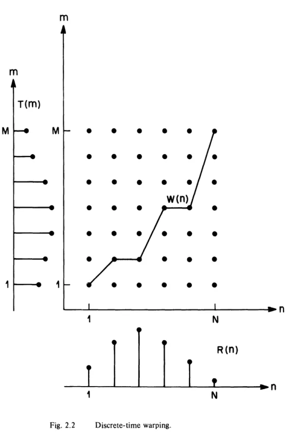
where d(R(n),T(w(m))) is the local distance between frame n of the reference and frame m = w(n) of the test. A typical path, w(n), is shown in Figure 2.2. It is important to notice that w(n) is restricted to begin at the point n = 1, m = 1, to pass through the grid of points

(n,m), where n and m are integers, and to end at the point n = N, m = M.

Although w(n) has been restricted to integer values, it is still functional in nature, i.e. for any n, the time alignment path passes through at most value of m. It is not unreasonable, however, that the best warping may not be functional. In this situation it is necessary to create a time warping procedure which maps both the reference pattern's time axis and the test pattern's time axis onto a common time axis. Such a procedure requires the use of two func-tions, i(k) and j(k), where k is the index of the common time axis. These two functions are used to map R(n) and T(m) to the common time axis, k, according to the rules

n = i(k), k = 1,2,...,K (2.3a)

m = j(k),

k = 1,2,...,K

(2.3b)

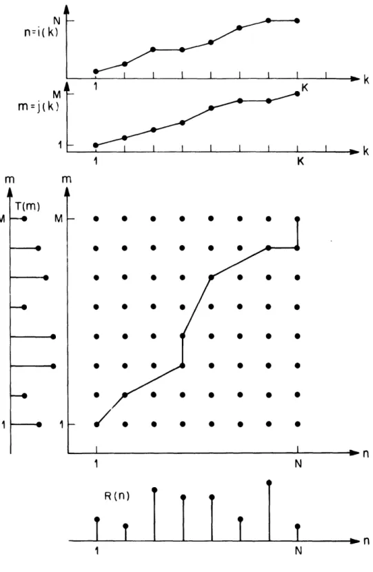
where K is the length of the common time axis. Figure 2.3 shows a typical example in which we plot i(k) and j(k) versus k, and in which we also show the resulting curve in (n,m) space. We see that, in (n,m) space, the resulting curve can be interpreted as a monotonically increas-ing path from the point (1,1) to the point (N,M) via several intermediate points. It is also

m

w(n)

* * i

N

N

Fig. 2.2 Discrete-time warping.

m

T(m)

i

i

i

I

R(n)

i

I I I I I I I I - t, I K . t I l ,I I | l I | 1 K

m

m

R(n)

Fig. 2.3 Time warping as path finding.

N

n=i(k)

m=j(k)

T(m)

clear that if the function

i(k)

m = j(k) = j(n) = w(n), i.e. the problem is equivalent to the discrete time version of the

problem given in Eq. (2.1). We will use the interpretation of time warping as finding an optimal path as the general framework for the remainder of this thesis.

2.2 Time Warping as Path Finding

Based on the discussion of the previous section, we see that for the interpretation of time warping as a path finding problem we must specify several features of the problem. The factors which are applicable to the path finding problem are the following:

1. Endpoint constraints - i.e. the way in which the path begins and ends.

2. Local continuity constraints - i.e. the possible types of motion (e.g. directions, slopes, etc.) of the path.

3. Global path constraints - i.e. the limitations on where the path can fall in the (n,m) plane. 4. Axis orientation - i.e. the effects of interchanging the roles of the test and reference

pat-terns.

5. Distance measures - both the local measure of similarity or distance between frames of the reference and test patterns and the overall distance function used to determine the optimal path.

In this section we discuss some possible (and hopefully reasonable) choices for each of the above factors for speech recognition applications.

2.2.1 Endpoint Constraints

Endpoint considerations for speech recognition fall into two broad categories based on whether the application is for connected words or for isolated words. We defer the question of how to handle endpoint constraints of connected words to Chapter 6 of this thesis. For isolated word recognition, endpoint detection is a relatively well-understood problem and several viable solutions have been proposed [8,9]. In the next three chapters we will be solely concerned with speech recognition systems which use simple isolated test utterances and which use reference

patterns consisting of isolated words. For time warping algorithms involving isolated utterances it is reasonable to assume that the endpoints of both the test and the reference patterns have been reliably determined. Given such an assumption, a time warping algorithm should be res-tricted to have all of its paths start at the point (1,1) (the first frame of both the reference and the test) and end at the point (N,M) (the final frame of both the reference and the test). In terms of the path notation we have

1i(1) = 1,1 j(1) = 1 (2.4a)

i (K) = N, j (K)

M.

(2.4b)

2.2.2 Local Continuity Constraints

Local continuity constraints are another important consideration for time warping in speech recognition systems. Local continuity constraints define what types of paths are allowable. For example, it would not be reasonable to allow a path for which a 10 to 1 expansion or compres-sion of the time axis occurs. Another consideration is the preservation of time order. The functions i(k) and j (k) should both be monotonically increasing, i.e.,

i(k+l) > i(k)

(2.5a)

j(k+l) > j(k).

(2.5b)

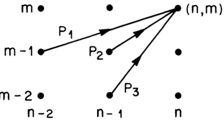
Local continuity constraints are easily expressed as simple local paths which may be pieced together to form larger paths. For example, to reach a point (n,m) it may be reasonable to have come from the points (n-l,m-1), (n-l,m-2) or (n-2,m-1). Such a set of legal paths may be viewed as shown in Figure 2.4, part a. Further restrictions may be placed on the local paths. For example, the path from (n-l,m-2) to (n,m) may be forced to pass through the point (n,m-1) and the path from (n-2,m-1) to (n,m) may be restricted to pass through the point (n-l,m). Such restricted paths are shown pictorially in part b of Figure 2.4 and are labeled as type I local constraints to distinguish them from other local constraints which will be defined later.

Local constraints for time warping may be formally expressed as a set of productions in a regular grammar. A production is a rule of the form

me

m-1 ()

m-2.

n-2

_n-1

*(n,m)

0

n

LEGAL PREVIOUS

P

n-2

n-1

POINTS

(n,mn)

n

TYPE I

LOCAL

CONSTRAINTS

Type I local constraints.

(a)

0

(b)

_m

m-1

m-2

(2.6) where r signifies the r'tl production and L (r) is the length of the r'l' production. The

interpre-tation of the (a ',P ('))'s in a production are that of the local changes (i.e. incremental changes) allowable in a path. The interpretation of a production, P,., used to reach a point (n,m) is as follows (proceeding from (n, n) back along the path'):

end point: (n,m)

1 ' point back: (n-a (', m-,8I 1)

2 "" point back: (n-at' -o2', m-13"' -P2

s"'

point back: (n-ia

m-,3

I

'))

s 'point back: (n-ya[",m-~fl'"')

/=1 /=1 L(,) L(r)

original

point: (n-

a ,

'm-

'),

or, in terms of the path functions of Eqs. (2.3),

k'

_{point: i(k) = n,}

_j(k)

_{= m}

(k-s) "' point:

i(k-s) = i(k) -a

'

j(k-s) = j(k)

-

God'"

As an example, the paths of Figure 2.4, part b, may be expressed by the three productions

P

-

(1,0) (1,1)

(2.9a)

P - (1,1) (2.9b)

PI

-

1. In time warping algorithms all paths are retrieved backwards from the end point (N,M) to (1,1). Paths are retrieved backwards because the entire path is not determined until the end is reached.

(2.8b)

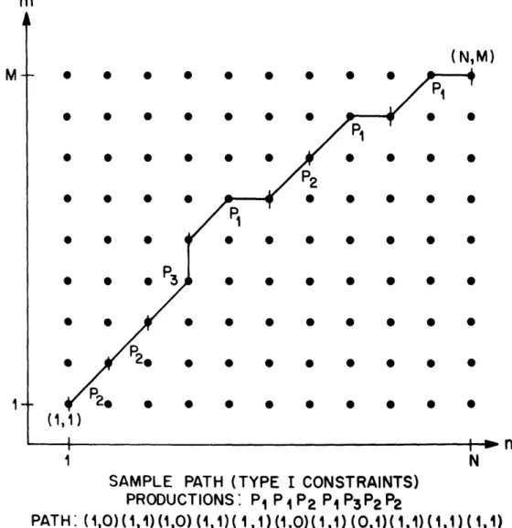
An entire path from the point (1,1) to the point (N,M) can be expressed as a sequence of pro-ductions tracing a path back from (N,M) to (1,1). Figure 2.5 shows an example of the path defined by the sequence of productions, P P P2 P P P P (traced backwards from (N,M) to (1,1)). The actual path from (N,M) back to (1,1) is given by substitution from Eqs. (2.9) into the sequence of productions to yield the sequence (1,0) (1,1) (1,0) (1,1) (1,1)

(1,0) (1,1) (0,1) (1,1) (1,1) (1,1).

Since a' 1and 13 '[' are simply the local changes in a path, the time ordering restrictions of

Eqs. (2.5) may be formulated as

(/"',/'> O. (2.10)

Also, restrictions on the degree of local compression and/or expansion can be incorporated into the local paths. The maximum and minimum amount of expansion (1/compression), denoted as Emax and Emin, can be obtained as

Emax =max a (2.1la)

L(r) L() (2.11a)

Em, =

a

am

I/"'

.

)

(2.11b)

For the paths of Figure 2.4b the maximum expansion is 2 and the minimum is 1/2.

Two other local continuity constraints with the same maximum and minimum slope of 2 and 1/2 respectively are shown in Figure 2.6, parts a and b. The productions associated with these local constraints are as follows:

Pf' - (2,1) (2.12a)

P, - (1,1) (2.12b)

PI - (1,2) (2.12c)

30

m

Fig. 2.5 Sample path.

A-

1-I N

SAMPLE PATH (TYPE I CONSTRAINTS)

PRODUCTIONS: Pi P 4 P2 P P3P2P2

PATH' (,0)(1,1)(1,0)(1,1}(t,1)(1,0(1,1(0,1)(1,1}(1,1}(t,1}

n-2

(n,m)

P1

n-1

n

TYPE

I

LOCAL CONSTRAINTS

n-2

(n,m)

n-I

n

TYPE

mI

LOCAL CONSTRAINTS

Fig. 2.6 Local constraints types II and III.

(a)

m

m-1

m-2

(b)

m

m-1

m-2

Pt - (1,0)(1,1)

(2.13a)

P H - (1,0)(1,2) (2.13b)

p __(1, -t 1) (2.13c)

P4- (1,2). (2.13d)

Type II local constraints are similar to type I, i.e. symmetric and come from the same points as type I, but type II constraints are lacking in the use of intermediate points. Type III constraints are somewhat different in that they are assymetric, using intermediate points in the x direction but not in the y direction. (Type II constraints are a production rule version of the local con-straints used by Itakura [6].) It should also be noted that all of the local concon-straints defined so far have a "memory" of two. That is, to reach a point (n,m) from a point (n',m') in one pro-duction it is necessary that n - n' K 2 and m - m' 2, i.e. the original point is no more than two units away in either axis. As we shall see in Section 2.3, such a limited "memory" (i.e. not infinite) is important in the efficient implementation of a path finding algorithm.

The research undertaken in this thesis involved the use of all three of the local constraints defined thus far. For ease of reference these different local constraints are referred to as types I, 1I and III, corresponding to the productions of Eqs. (2.9), (2.12) and (2.13) respectively. It should be noted that type I local constraints are exactly those specified by Sakoe and Chiba using a P value of 1, corresponding to a maximum slope of 2 and a minimum slope of 1/2 [10]. Sakoe and Chiba found that this slope constraint was optimal and, for the most part, we will use only a maximum slope of 2 and a minimum slope of 1/2.

2.2.3 Global Path Constraints

Another factor in time warping for speech recognition is that of global range constraints. Global range constraints specify which points (i(k),j(k)) are allowed to occur within a legal path. These points constitute the global range. Global range constraints arise naturally as a result of local continuity constraints. Local continuity constraints force certain points of the (n,m) plane to be excluded from legal paths because they would require excessive expansion or compression of the time scales. For example, the point (2,10) would be illegal (under the local

constraints described thus far) because it would require a 9 to 1 expansion to be reached from the point (1,1). The global constraints arising from local continuity constraints may be expressed as

1 +

( (k)-)

j(k)

1

+

E+

ma(i(k)-l1)

(2.14a)

Emax

M + Emax(i(k)-N)

<

j(k)

<

M + (i(k)-N)

(2.14b)

Emax

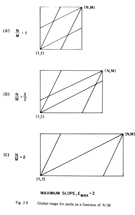
where Emax is the maximum allowable expansion (and En,,i=l/Enax). The first constraint of Eq. (2.14) may be interpreted as restricting the range of legal points to those which do not require excessive expansion or compression in order that they be reached from the point (1,1). The second constraint of Eq. (2.14) eliminates those points which would necessitate excessive expansion or compression in order to eventually reach the point (N,M). One useful way to view these constraints is as limiting all legal paths to fall within the bounds of the parallelogram of Figure 2.7. The size of this region depends strongly on the values of N and M. Figure 2.8 shows the affects of the successive nature of N/M of 1, 3/2 and 2 on the global range of paths for a value of maximum slope of Emax = 2. The range of legal paths decreases quickly with

increasing N/M (or MIN). These effects are often significant in speech recognition systems in which there is a high variability among replications of the same utterance (i.e. M/N approaches or exceeds 2, or falls below 1/2).

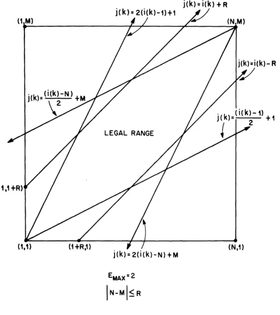
Another possible restriction on the global range has been proposed by Sakoe and Chiba [4]. They proposed that the absolute difference, i (k)-j(k) , be limited to be less than or equal to

some integer value, R:

jI(k)-j(k)l < R.

(2.15)

This type of restriction may be interpreted as imposing a limit on the absolute time difference which can be allowed between frames, i.e. frame i (k) of the reference pattern is res-tricted to fall within R Ts seconds of frame j(k) of the test pattern, where T is the sampling period for frames (typically 10 to 30 milliseconds). Pictorially, the restriction of Eq. (2.15) cuts

34

j(k)=2(i(k)-l)

+

EMAX 2

N 3 M 2 (N,M) (1,1) (N,M) (1,1) (C) N M (1,1)

MAXIMUM SLOPE, _{EMAX =2}

Fig. 2.8 _{Global range for paths as a function of N/M.}

(a) N

M

(b)

36 off the corners of the parallelogram of Figure 2.7, as illustrated in Figure 2.9.

For notational purposes we will refer to those time warping algorithms which use an abso-lute time difference range constraint as range - limited algorithms and those which do not use

Eq. (2.15) as a range constraint as range - unlimited algorithms. 2.2.4 Axis Orientation

Axis orientation is another important consideration in a time warping algorithm. Axis orien-tation determines if the functions of Eqs. (2.3) are used or if the inverse set of equations is

used, i.e.

n = j(k), k = 1,2,...,K (2.16a)

m = i(k), k = 1,2,...,K (2.16b)

The differences between Eqs. (2.3) and Eqs. (2.16) can be important when the local con-straints are not symmetric, as with type III local concon-straints, or when the distance function for determining an optimal path is not symmetric. In general, we will refer to the paths of Eqs. (2.3) as "reference along the x-axis," as in Figure 2.3, and those paths of Eqs. (2.16) as "test along the x-axis." (For convenience, we will use Eqs. (2.3) in all our discussions, unless other-wise noted.)

2.2.5 Distance Measures

The final consideration in the specification of a time warping algorithm is a distance function which is used to determine the optimal path. A typical distance function has the form

d(i(k),j(k)) W(k)

D(i(k),j(k))= &-l (2.17)

where D(i(k),j(k)) is the total distance along the path of length K (i.e. K-I arcs or K pairs

(i(k),j(k))), defined by the functions i (k) and j(k). 2 The overall distance is given as a nor-malized, weighted sum of local distances where d(i(k),j(k)) is the value of the local distance

2.

Technically, D(i(k),j(k)) is a functional, that is, a function of a set of functions, i(k) and j(k), but, for sake of simplicity we will refer to it as a function.

EMA_X 2

|N-M R

Fig. 2.9 _{Global range for paths with range limiting.}

-R

+1

metric at frames i(k) of the reference and

ji

(

is a normalization factor which, in general, depends on the weighting function used. The best path is the set of functions i(k), j(k), k = 1,2,...,K which minimize the distance function. The total distance between a test and a reference, D, is defined to be the minimum distance achieved by the time warping algorithm, i.e.

D

=

min

(D(i(k),j(k))).

(2.18)

(K,i(k ),j(k ))

To define the total distance function we must define d(i(k),j(k)), W(k) and N(W1/). Choice of the local distance metric, d(i(k),j(k)) is dependent on the feature set used to create both the test and the reference patterns. Typical choices include a log spectral difference for energy measurements, a Euclidean distance for cepstral coefficients and a log likelihood ratio for LPC coefficients [6]. Thus, the local distance metric is independent of the particular time warping algorithm. The weighting function and the normalization are not, however, indepen-dent of the time warping algorithm.

Typically, a weighting function depends only on the local paths. For example, the weight used on the path from the point (i(k-l),j(k-l)) to the point (i(k),j(k)) depends only on

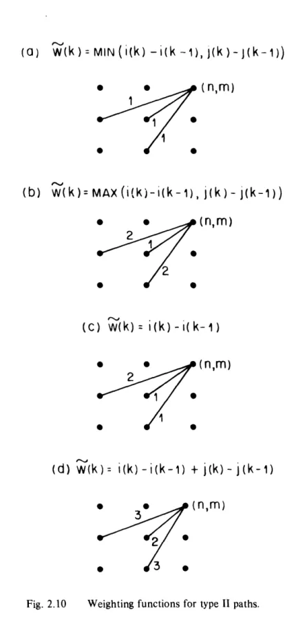
i (k) - i(k-1) and j(k) - j(k-1). Typical weighting functions which are used include

W(k) = min(i(k)-i(k-l),j(k)-j(k-1))

(type a)

(2.19a)

W(k) = max(i(k)-i(k-1),j(k)-j(k-))

(type b)

(2.19b)

(k) = i(k) -

i(k-1)

W(k) = i(k) - i(k-1) + j(k) -

j(k-1)

(type d)

.

(2.19d)

Weighting functions c and d have been proposed by Sakoe and Chiba [10] as weighting all the samples of the x-axis pattern equally (type c) or as weighting all samples of both the x and y-axis patterns equally (type d). Weighting function a weights all segments of a path equally, regardless of their length and weighting function b weighs shorter segments less than longer segments. As we shall see, weighting functions c and d have no particular bias in their choice

of paths, weighting function a favors longer paths over shorter paths and weighting function b favors shorter paths over longer paths. For initialization purposes, i(O) and j(0) are defined to

be 0 and thus W(1) = 1 for weighting functions a, b and c and W(1) = 2 for weighting func-tion d.

A pictorial representation of these various weighting functions as applied to type II paths is given in Figure 2.10. The number labeling the various arcs are the weighting functions associ-ated with paths that lie along those particular arcs. Figure 2.11 shows two different representa-tions of the various weighting funcrepresenta-tions as used with type I paths. The left hand column uses the weighting functions exactly as defined. In the right hand column a smoothing process has been applied. Smoothing is a procedure in which multiple segment local paths have their weighting functions averaged. This process was first used by Sakoe and Chiba [10] to prevent certain anomolies such as the left hand side of Figure 2.11, part a, in which some arcs have a

zero weight thus allowing a loss of information from local distances which are ignored.

In Figure 2.12 we show an example of a typical type II path with a type d weighting func-tion. In this example the arcs along the path are labeled with the corresponding weighting functions, the values of N, M and K are 11, 9 and 8 respectively and the overall distance is given by

D(i(k),j(k)) = [2d(1,1)+3d(3,2)+2d(4,3)+3d(5,5)

(2.20)

+ 3d(7,6)+3d(9,7)+2d(10,8)+2d( 1,9)]/N( Wd)

where N( Wd) is the normalization associated with weighting function d.

The choice of N(W) is typically made such that D(i(k),j(k)) is an average local distance along the path defined by the functions i(k) and j(k). As such, the natural choice for N( W) is the sum

K

N(W) = I W(k).

(2.21)

k-1

40

(a)

w(k

) MIN

(i (k) -(k -), (k)-j(k-1))

(n,m)

(b) w(k)=

MAX

(ikj-i(k-1),

j(k)

j(k-1))

(n,m)

(c)

W(k)=

i(k)

-i( k-1 )

(n,m)

(d) w(k)=

i(k)

-i(k-1) +

j(k)

- j(k-1)

(n,m)

Fig. 2.10 Weighting functions for type II paths. I

(n,m)

/2

(b) w(k)

=MAX(i(k)-

i(k-1),j(k)-j(k-1))

(n,m)

(d) W(k)=

i(k)-i(k-l) + j(k)-j(k-i)

(n,m)

3/2

Fig. 2.11 Weighting functions for type I paths.

1

n,m)

(n,m)

(n,m)

(n,m)

3/2

(a) W(k = MIN ( i (k ) - I (k - q, j (k) - j (k - i))

m

(11,9)

3

2/

oIn

N=11,M9

K=8

W(k)=

_{i(k)-i(k-) + j(k) - j(k-l)}

D(i(k),j(k))=

_{[2d(1,1)+ 3d(3,2) +2d(4,3)+ 3d(5,5)+ 3d(7,6) +}

3d(9,7) + 2d(10,8) + 2d(11,9)] /N(Wd)

Fig. 2.12 Sample path with distance measure.

I

W. m ~ A

-K

N(W,.) =

(i(k)-i(k-1))

= i(K) - i(O) = N

(2.22a)

N(Wd) = I (i(k)-i(k-)+j(k)-j(k-1))

(2.22b)

= i(K) - i(O) + j(K) - j(O) = N + M.

However, for weighting functions a and b the value of Eq. (2.21) is not a constant, but instead depends upon the path chosen. Figure 2.13 shows two simple paths, Path 1 and Path 2, for the case N = M. Path 1 is the straight line path of slope = 1 from (1,1) to (N,M). Path 2 has two sections, the first of which has a slope = 1/2 and the second of which has a slope = 2. If N(Wi) is defined as in Eq. (2.21) then the values of N(W) for weighting function a are given approximately by

Path 1: N(W)= N (2.23a)

Path 2: N(Wa) = 2N (2.23b)

3

The value of Eq. (2.23a) is generated by N segments of weight 1 and the value of Eq. (2.23b) is generated as 2N/3 segments of slope 1/2 (average value of Wa(k)=1/2) and N/3 segments of slope 2 (average value of Wa (k)= 1) for a total of

N(Wa,)=1/22N/3 + N/3 = 2N/3. For weighting function b the values of N(W) as defined

by Eq. (2.21) are given in an analogous manner by

Path 1: N ( Wb) = N (2.24a)

Path 2: N(Wb) = 4N (2.24b)

3

In section 2.3 we will show that, in order to solve for the optimal path efficiently, it is neces-sary that N(W) be independent of path. Thus, for computational convenience, we define N ( W) as follows:

N(W,) = N

(2.25a)

N(Wb)

44

z

Z

z

N(W

-

N + M.

(2.25d)

An important consideration of the performance of a time warping algorithm arises from the definitions of Eqs. (2.25). Use of these definitions can create situations in which certain paths are favored over others. An algorithm in which such a situation can arise is said to be biased.

Formally, a time warping algorithm is unbiased when the following condition is true:

if d(i(k),j(k)) = d then D(i(k),j(k)) = d,

(2.26)

i.e. if the local distance is independent of i(k) and j(k) then the global distance function is also independent of i (k) and j(k). Equivalently, if the local distance is independent of the path chosen then there is no preferred path to be chosen.

By direct substitution of d(i(k),j(k)) = d into Eq. (2.17) we obtain K

d Wi(k)

D(i(k)j(k)) =

_g

_(,'(2.27)

(2.27)

Thus, condition (2.26) is true if and only Eq. (2.21) is true, and is thus true for weighting functions c and d by Eqs. (2.22). However, condition (2.26) is not true for weighting func-tions a and b. Using the paths of Figure 2.13 we get the following values for D(i(k),j(k)) using weighting function a,

Path 1: D(i(k),j(k)) = d (2.28a)

Path 2: D(i(k),j(k)) = 2d (2.28b)

3

and using weighting function b,

Path 1: D(i(k),j(k)) = d (2.28c)

Path 2: D(i(k),j(k)) =

_.

_(2.28d)

3

Thus, we see that weighting function a has a preference for the longer path, Path 2 over Path 1 (lower global distance function) and that weighting function b has a preference for the shorter path, Path 1 over Path 2. This form of bias may be expected to be detrimental to the performance of a time warping algorithm because bias may prevent the time warping algorithm

46 from following the truely accurate path.3

2.2.6 Solution for the Optimal Path

In Tables 2.1, 2.2, 2.3 and 2.4 we summarize the various features of a time warping algo-rithm as we have presented them in the previous sections. Once all of the factors for a time warping algorithm have been specified, the optimal path under these conditions may be found. Several methods exist for finding this optimal path. One method is exhaustive search of all possible paths from (1,1) to (N,M). This is, in general, prohibitively expensive and time con-suming (on the order of 2 ' operations). Another approach would be to apply Dykstra's path finding algorithm to the problem [11]. While faster than exhaustive search methods, this method also can be very time consuming for large values of N and M (order of N2M2 opera-tions). A better approach was suggested by Sakoe and Chiba [4]. They proposed the use of dynamic programming to efficiently solve the problem. Dynamic programming is an efficient method to apply because dynamic programming successively builds longer optimal paths from smaller optimal paths [5] (order of NM operations). In the next section we discuss how dynamic programming is applied to our problem.

2.3 Dynamic Time Warping

Two basic principles are involved in dynamic programming as applied to time warping, or dynamic time warping (DTW), as it is referred to. The first principle is that a globally optimal path is also locally optimal. The globally optimal path is the path which minimizes the weighted distance from (1,1) to (N,M) according to Eq. (2.18). A locally optimal path from a point (n',m') to a point (n,m) is the path which minimizes the weighted distance from (n',m') to (n,m). To say that the globally optimal path is also locally optimal is equivalent to the state-ment that for any two points (n',m') and (n,m) along the globally optimal path, the locally optimal path from (n',m') to (n,m) is exactly the subsection of the globally optimal path from

(n',m') to (n,m). This must be true because, if there were a better locally optimal path from 3. An examination of the literature on speech recognition reveals that White and Neely [3] used weighting function b. Such a situation may account for the lack of improvement in recognition scores using a nonlinear time warping as compared to a linear time warping for the alphabet-digits vocabulary.

LOCAL CONSTRAINTS

I IL~··~~·~L·~

TYPE

I

PICTORIAL

PRODUCTIONS

I

---

I

P-i -0.-(t,0)(t)

P

3

-.- (0,1)(

1)

P

a- (2,1)

P

-

(1,

)

P

--- (, 2)

I

I P

-

(1,O)(1,I)

IP2--(0)(,2)

I P3

*(1,t)

I P4-

4,2)

Endpoint Constraints

i(1) = 1, i(K) = N

j(l) = 1,

tj(K)

Global Constraints

From Local Constraints:

(i(k)-l)

EOWJ

+

I < j(k) <

Emax(i(k)-l) +

Emx

Emx(i(k)-N) + M

<.j(k) <

-

(i(k)-N) + M

En,ax - Maximum Slope

Range Limited:

i(k)- R

j(k)

i(k) + R

Table 2.2

Axis Orientation Reference along X-axis:

Test along X-axis:

n = i(k), = j()

n =

j(W),

Overall Distance Measure

i(k),.j(k)) ;(k)

N( W) Table 2.3

Axis Orientation and Distance Measure

- 111111l I

( (A ), j/ A),K )

..

~~~~

50 Weighting Functions

Type Definition Normalization

N N( W) a W(k) = min(i(k)-i(k-1), N

.i(k)-j(k-1))

j(k -,j(-1)

N+M

+

_i(k)

(n',m') to (n,m) it could be substituted into the globally optimal path with a corresponding improvement in the globally optimal path.

The other principle involved in a dynamic programming implementation of a time warping algorithm is the dependence of the best path to a point (n,m) only on (n',m') such that

n' < n (2.29a)

m' < m. (2.29b)

This follows from the monotonicity restriction of Eqs. (2.5).

As a result of these two principles, it is possible to create a partial accumulated distance function D(n,m). DA(n,m) is the accumulated distance from the point (1,1) to the point (n,m) using the best possible path to reach (n,m), i.e.

DA(n,m)

min

d (i(k),j(k))

(k)

( ),j ), A") kAI=1

where K' is the length of the path from (1,1) to (n,m) and where

i(1) = 1, i(K') = n (2.31a)

j(1) = 1, j(K') = m. (2.31b)

Since DA(n,m) depends only on the paths from (1,1) to (n,m) and since the optimal path to (n,m) depends only on those points (n',m') which satisfy Eqs. (2.29), DA(n,m) can be defined recursively in terms of (n',m') by

D4(n,m) = min[DA (n',m')+d((n',m'),(n,m))]

(2.32a)

DA (1,1) = d (1,1) W(1) (2.32b)

where d((n',m'),(n,m)) is the weighted distance from (n',m') to (n,m), i.e. I.-I

d((n',m'),(n,m))

=

d (i(K'-l),j (K'-l)) J/(K'I)

(2.33)

I=0