HAL Id: tel-01056825
https://tel.archives-ouvertes.fr/tel-01056825
Submitted on 20 Aug 2014
HAL is a multi-disciplinary open access archive for the deposit and dissemination of sci-entific research documents, whether they are pub-lished or not. The documents may come from teaching and research institutions in France or abroad, or from public or private research centers.
L’archive ouverte pluridisciplinaire HAL, est destinée au dépôt et à la diffusion de documents scientifiques de niveau recherche, publiés ou non, émanant des établissements d’enseignement et de recherche français ou étrangers, des laboratoires publics ou privés.
Multi-resolution physiological modeling for the analysis
of cardiovascular pathologies
David Ojeda Avellaneda
To cite this version:
David Ojeda Avellaneda. Multi-resolution physiological modeling for the analysis of cardiovas-cular pathologies. Signal and Image processing. Université Rennes 1, 2013. English. �NNT : 2013REN1S187�. �tel-01056825�
ANNÉE 2013
THÈSE / UNIVERSITÉ DE RENNES 1
sous le sceau de l’Université Européenne de Bretagne
pour le grade de
DOCTEUR DE L’UNIVERSITÉ DE RENNES 1
Mention : Traitement du Signal et Télécommunications
École doctorale Matisse
présentée par
David Ojeda Avellaneda
Préparée à l’unité de recherche INSERM, U1099
Laboratoire de Traitement du Signal et de l’Image
UFR ISTIC: Informatique et Électronique
Multi-resolution
physiological
modeling for
the analysis of
cardiovascular
pathologies
Thèse à soutenir à Rennes le 10 décembre 2013
devant le jury composé de :
Catherine MARQUE
PU à l’Université de Technologie Compiègne/Rapporteur
Vanessa DIAZ-ZUCCARINI
Lecturer à University College London/Rapporteur
Michel ROCHETTE
Directeur de Recherche chez ANSYS / Examinateur
Jean-Philippe VERHOYE
PH/PU à l’Université de Rennes 1/Examinateur
Alfredo I HERNÁNDEZ
Chargé de Recherche INSERM, HDR/Directeur de thèse
Virginie LE ROLLE
Abstract
This thesis presents three main contributions in the context of modeling and simulation of physiological systems. The first one is a formalization of the methodology involved in multi-formalism and multi-resolution modeling. The second one is the presentation and improvement of a modeling and simulation framework integrating a range of tools that help the definition, analysis, usage and sharing of complex mathematical models. The third contribution is the application of this modeling framework to improve diagnostic and therapeutic strategies for clinical applications involving the cardio-respiratory system: hypertension-based heart failure (HF) and coronary artery disease (CAD). A prospective application in cardiac resynchronization therapy (CRT) is also presented, which also includes a model of the therapy. Finally, a final application is presented for the study of the baroreflex responses in the newborn lamb. These case studies include the integration of a pulsatile heart into a global cardiovascular model that captures the short and long term regulation of the cardiovascular system with the representation of heart failure, the analysis of coronary hemodynamics and collateral circulation of patients with triple-vessel disease enduring a coronary artery bypass graft surgery, the construction of a coupled electrical and mechanical cardiac model for the optimization of atrio ventricular and intra ventricular delays of a biventricular pacemaker, and a model-based estimation of sympathetic and vagal responses of premature newborn lambs.Résumé en français
Les maladies cardiovasculaires représentent la principale cause de mortalité chez les adultes (30% des décès enregistrés en 2004) dans l’ensemble des pays membres de l’Organisation Mondiale de la Santé (WHO, 2008). Les processus impliqués dans les maladies cardiovasculaires sont le plus souvent complexes et multifactoriels. C’est le cas de l’insuffisance cardiaque (IC) qui est une pathologie présentant l’une des plus fortes prévalences dans le monde. Dans l’IC, la réduction significative du débit cardiaque est due à des modifications des propriétés mécaniques du myocarde et est parfois liée à une altération de l’activation électrique (désynchronisation intra ou inter-ventriculaire). De nombreux mécanismes (nerveux ou hormonaux) de régulation sont alors activés, couvrant ainsi des échelles de temps très différentes (de la seconde à la semaine). Bien que ces mécanismes puissent compenser les conséquences de l’IC à court terme, leurs effets peuvent devenir délétères à moyen et long terme, accentuant ainsi les dysfonctionnements ventriculaires. On peut notamment observer une augmentation de la précharge et de la postcharge, un remodelage cardiaque, des œdèmes pulmonaires ou périphériques, une baisse du débit rénal et des difficultés respiratoires.L’étude de telles pathologies multifactorielles nécessite l’acquisition de données cliniques susceptibles de pouvoir fournir des indicateurs de l’état du patient. Or l’analyse de ces données peut s’avérer complexe car celles-ci peuvent i) provenir de différentes modalités d’acquisition, ii) être associées à différents organes, iii) couvrir différents intervalles temporels, et iv) être nombreuses et difficile à analyser et interpréter. Dans ce contexte, une approche à base de modèle pourrait être utile à l’analyse de données cliniques et à la compréhension des évènements impliqués dans un état pathologique. En effet, l’utilisation de la modélisation dans ce contexte peut constituer une aide à l’analyse des phénomènes observés cliniquement à partir des hypothèses incluses dans le modèle et à la compréhension du fonctionnement d’un système physiologique. Par ailleurs, l’utilisation de modèles peut être utile à la prédiction du comportement futur (et des pathologies éventuelles pouvant survenir) et à l’assistance pour la définition de nouvelles thérapies, par exemple dans le cadre des thérapies de resynchronisation cardiaque.
Plusieurs modèles des différents composants de systèmes physiologiques (activité cardiaque, respiration, fonction rénale, système nerveux autonome, etc.) ont été proposés dans la littérature à différents niveaux de détail. L’intégration de ces différents modèles peut permettre de mieux analyser et de mieux comprendre les processus physiopathologiques complexes résultant de leur interaction. Au moins deux types d’intégration peuvent être identifiés : l’intégration structurelle (ou verticale) et l’intégration fonctionnelle (ou horizontale). La plupart des travaux présentés
iv Résumé en français
aujourd’hui sont basés sur une intégration structurelle exhaustive (de la cellule à l’organe, par exemple), impliquant des modèles complexes, en termes du nombre des variables d’états représentées, d’éléments impliqués, etc. Ces modèles conduisent à des simulations lourdes et sont difficiles à analyser, à identifier et à exploiter dans un contexte pratique. Les modèles qui visent une intégration horizontale fonctionnelle, couplant différents sous-systèmes physiologiques, sont moins présents dans la littérature. Même si ces modèles sont plus aisés à manipuler (numériquement et mathématiquement), ses éléments constituants ne disposent pas du niveau de détail suffisant pour expliquer certains modes de fonctionnement du système à analyser.
Un moyen de contourner ces problèmes est de représenter différentes fonctions à des échelles distinctes, dans une approche multi-résolution. Cela implique la création de modèles intégrant plusieurs composantes physiologiques développées à différents degrés de complexité structurelle en fonction de l’objectif clinique. Cependant, ces modèles peuvent présenter des formalismes hétérogènes (c’est-à-dire modèles continus d’équations différentielles ; modèles discrets, tels qu’au-tomates cellulaires, etc.), plusieurs niveaux de résolutions ou différentes dynamiques temporelles. Le couplage de modèles hétérogènes implique des difficultés techniques et méthodologiques tel que :
– la création d’un environnement approprié basé sur un modèle de base (ou « core model ») modulaire et sur des outils spécifiques de modélisation et de simulation de modèles couplés hétérogènes,
– la définition d’une méthode d’interfaçage pour le couplage de ces modèles hétérogènes préservant la stabilité et les caractéristiques essentielles de chaque modèle.
Cette thèse propose des solutions afin de contourner ces problèmes et représenter différentes fonctions à des échelles distinctes, dans une approche multi-résolution, en définissant les interfaces nécessaires à l’intégration de modèles. L’approche proposée pour l’interfaçage de modèles hétéro-gènes intègre : i) la restructuration des modèles devant être couplés, ii) l’analyse de sensibilité réalisée sur les modèles, et iii) la définition des transformations nécessaires sur les entrées/sorties. L’implémentation de cette approche de modélisation intégrative nécessite l’utilisation d’une librairie de simulation adaptée. Dans ce cadre, un environnement de modélisation et de simula-tion, précédemment développé au laboratoire, appelé « Multiformalism Modeling and Simulation Library » (M2SL) a pu être utilisé et amélioré. Des outils d’analyse des paramètres (analyses de sensibilité et identification de paramètres) ont notamment pu être ajoutés aux fonctionnalités existantes dans M2SL permettant ainsi de mieux appréhender les caractéristiques de modèles hétérogènes et de faciliter le couplage avec des données cliniques.
Dans cette thèse, la méthodologie concernant l’utilisation de modèles multi-résolution en physiologie a pu être appliquée à plusieurs cas cliniques : i) l’étude des conséquences court et moyen terme de l’insuffisance cardiaque, ii) la modélisation spécifique-patient des coronaires pour l’étude de la circulation collatérale, iii) l’analyse spécifique-patient de modèles cardiovasculaires pour l’optimisation de thérapies de resynchronisation cardiaque, et iv) l’évaluation des voies sympathique et vagale chez l’agneau nouveau-né.
Résumé en français v
entre un modèle d’intégration horizontal couplé avec un modèle de ventricule plus résolu. Le travail pionnier de Guyton (Guyton et al., 1972) sur l’analyse de l’ensemble de la régulation du système cardio-vasculaire a été utilisé et les ventricules non-pulsatiles du modèle de Guyton ont été remplacés par des représentations pulsatiles des ventricules sous forme d’élastance qui s’exécutent à une échelle temporelle plus réduite. Des analyses de sensibilité ont notamment été réalisées pour comparer le modèle original et le modèle pulsatile. Par ailleurs, un épisode d’IC congestive a pu être simulé pour observer les variations des variables de régulation à court et moyen terme. Les variations caractéristiques des pressions artérielles systolique et diastolique ont notamment été observées, ce qui n’est pas possible avec le modèle original.
Ensuite, le cadre de modélisation et de simulation proposé a pu être appliqué à l’étude de la circulation coronarienne afin d’analyser des données cliniques obtenues durant des procédures de pontage coronarien. L’analyse des paramètres du modèle a permis de mettre en évidence l’importance de la circulation collatérale qui est un réseau de vaisseaux alternatifs se développant pour compenser la diminution du flux sanguin du réseau coronaire en cas de sténoses significatives. L’apport principal de ce travail est la création de modèles spécifique-patient dans le cas d’atteinte tritronculaire. Les données cliniques obtenues durant les pontages de dix patients ont pu être reproduites de manière satisfaisante avec le modèle et le développement des vaisseaux collatéraux a pu être évalué.
Une autre application clinique concerne l’étude de la perte de synchronisation cardiaque chez 25% à 50% des patients souffrant d’IC. Dans ce cas, une thérapie de resynchronisation cardiaque (CRT), qui consiste en l’implantation d’un pacemaker, peut être utilisée pour stimuler l’activité électrique cardiaque de manière à restaurer la coordination atrio-ventriculaire et intra-ventriculaire. Le modèle utilisé pour cette application clinique intègre : i) un modèle macroscopique de l’activité électrique cardiaque, ii) un modèle mécanique des ventricules et des oreillettes, et iii) des modèles des circulations systémique et pulmonaire. Le modèle complet intègre donc les activités électrique et mécanique cardiaques basées sur des formalismes différents. Cette application comporte deux apports principaux : la présentation de différentes analyses de sensibilité des paramètres du modèle mettant en évidence les paramètres systoliques ventriculaires, les paramètres reliés à la précharge et ceux en lien avec la description des propriétés diastoliques des ventricules. Ces paramètres ont des effets importants sur les indicateurs cliniques utilisés pour l’optimisation de la CRT ; la création de modèles spécifique-patient de sujets traités par CRT.
La dernière application clinique traitée dans cette thèse concerne l’analyse de l’activité du baroréflexe en néonatologie. En effet, l’activité autonomique est fortement impliquée dans les mécanismes qui mènent aux phénomènes d’apnée-bradycardie observés chez certains nouveau-nés. En effet, le baroréflexe est particulièrement immature durant les premiers jours de vie, particulièrement dans le cas de la prématurité, et il peut être intéressant d’évaluer les activités sympathique et vagal afin de mieux comprendre les mécanismes sous-jacents. Pour mener cette étude, un protocole expérimental a été défini en partenariat avec l’Université de Sherbrooke. Ce protocole a permis l’acquisition de signaux expérimentaux sur 4 agneaux nouveau-nés pendant des manœuvres d’activation du baroréflexe. Une identification récursive des paramètres du modèle
vi Résumé en français
de baroréflexe a pu être réalisée de manière à évaluer les variations des activités des voies vagale et sympathique pendant des injections de vasoconstricteur et de vasodilatateur.
Ainsi, les quatre applications cliniques traitées dans cette thèse mettent en évidence l’ap-plicabilité de la méthode d’intégration de modèles multi-résolution en physiologie. Un apport majeur de cette thèse est la formalisation et la généralisation de la méthodologie nécessaire à cette approche. Cette analyse théorique est accompagnée d’améliorations significatives des outils de modélisation et de simulation précédemment développés au laboratoire. Ces améliorations concernent notamment l’exécution de modèles mathématiques complexes et hétérogènes, ainsi que l’analyse et l’identification des paramètres de ces modèles. Ces outils sont centralisés dans M2SL qui est déjà utilisé dans différents laboratoires et est listé comme l’un des logiciels de simulation dans le réseau d’excellence « Virtual Physiological Human » (VPH NoE). L’application de ces outils pour la modélisation et l’analyse de systèmes physiologiques montre la pertinence de l’approche pour l’étude de problèmes cliniques concrets.
Contents
Abstract i
Contents vii
1 Introduction 1
References . . . 3
2 Modeling and Simulation 5 2.1 Modeling and simulation concepts . . . 5
2.2 General modeling and simulation framework . . . 8
2.2.1 Experimental frame and system specification . . . 9
2.2.2 System description . . . 12
2.2.3 Simulation . . . 14
2.2.3.1 Multi-formalism simulation . . . 16
2.2.4 Parameter analysis . . . 17
2.2.5 Validation . . . 19
2.3 Modeling and simulation in physiology . . . 20
2.3.1 Integrative modeling in physiology . . . 21
2.4 Conclusion . . . 24
References . . . 24
3 Contribution to multi-resolution modeling in physiology 27 3.1 Notation and problem statement . . . 28
3.2 Proposed sub-model interfacing approach . . . 29
3.2.1 Identification of the interaction variables in models MC, MRand MD . . 30
3.2.2 Whole-model and module-based sensitivity analyses . . . 32
3.2.3 Input-output coupling and temporal synchronization of heterogeneous models 32 3.3 Input-output model coupling . . . 33
3.4 Temporal synchronization of heterogeneous models . . . 34
3.5 Conclusion . . . 35
References . . . 36 4 Novel tools for multi-formalism modeling, simulation and analysis 39
viii Contents
4.1 Multi-formalism modeling and simulation . . . 39
4.1.1 Modeling and simulation tools: state of the art . . . 39
4.1.2 Proposed approach: Creation of a custom multi-formalism modeling and simulation library . . . 43
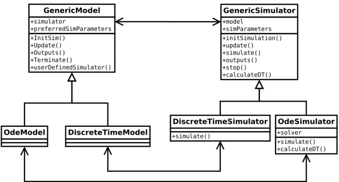
4.1.2.1 Model representation . . . 44
4.1.2.1.1 Algebraic equations models . . . 46
4.1.2.1.2 Ordinary differential equations models . . . 47
4.1.2.1.3 Discrete time models . . . 47
4.1.2.2 Simulator representation . . . 47
4.1.2.2.1 Algebraic equations simulator . . . 48
4.1.2.2.2 Ordinary differential equations simulator . . . 49
4.1.2.2.3 Discrete-time simulator . . . 50
4.1.2.2.4 User-defined simulators . . . 50
4.1.2.3 Transformation objects representation . . . 50
4.1.2.4 The simulation loop . . . 51
4.1.2.5 Adaptive simulation and synchronization . . . 53
4.1.2.6 Additional tools . . . 54
4.1.2.6.1 Sensitivity analysis tools . . . 55
4.1.2.6.2 Parameter identification tools . . . 55
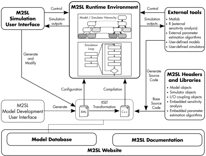
4.1.2.6.3 User interface . . . 56
4.1.2.6.4 M2SL website . . . 57
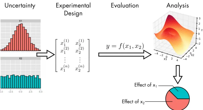
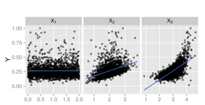
4.2 Sensitivity Analysis . . . 57
4.2.1 Local sensitivity analysis . . . 60
4.2.2 Global sensitivity analysis . . . 60
4.2.3 Screening methods . . . 63 4.2.4 Proposed approach . . . 64 4.3 Parameter identification . . . 65 4.3.1 Deterministic approaches . . . 66 4.3.2 Stochastic approaches . . . 67 4.3.2.1 Evolutionary algorithms . . . 68 4.3.3 Multiobjective optimization . . . 69 4.3.4 Proposed approach . . . 71 4.3.4.1 Objective functions . . . 72 4.3.4.2 Individual representation . . . 73 4.3.4.3 Population initialization . . . 73 4.3.4.4 Selection algorithm . . . 73
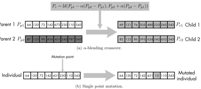
4.3.4.5 Reproduction: crossover and mutation algorithms . . . 74
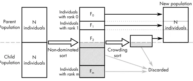
4.3.4.6 Non-dominated Sorting Genetic Algorithm (NSGA-II) . . . 74
4.4 Conclusion . . . 75
Contents ix
5 An example of multi-resolution integration: The Guyton model 81
5.1 Heart failure . . . 82
5.2 Problem statement . . . 83
5.3 Implementation of the Guyton model in M2SL . . . 83
5.3.1 The Guyton models . . . 84
5.3.2 Guyton Model implementation . . . 86
5.3.3 Verification . . . 86
5.4 Optimization of the temporal coupling . . . 88
5.5 Integration of pulsatile ventricles: a multi-resolution approach . . . 88
5.5.1 Coupling the Guyton and the pulsatile models . . . 89
5.5.2 Identification of the controller parameters . . . 93
5.5.3 Sensitivity Analysis . . . 93
5.5.4 Parameter identification and sensitivity analysis results . . . 94
5.6 Simulation of an acute decompensated heart failure (ADHF) . . . 95
5.7 Conclusion . . . 96
References . . . 97
6 Patient-specific modeling and parameter analysis of the coronary circulation 101 6.1 Coronary circulation . . . 101
6.1.1 Physiopathological aspects . . . 101
6.1.1.1 Collateral circulation . . . 104
6.1.2 Modeling coronary vascular dynamics: state of the art . . . 104
6.2 Problem statement . . . 105
6.3 Materials and methods . . . 106
6.3.1 Clinical measurements . . . 106
6.3.2 Model description . . . 107
6.3.3 Sensitivity analysis . . . 111
6.3.4 Parameter identification . . . 112
6.3.4.1 Previous approaches . . . 112
6.3.4.2 A multiobjective optimization approach . . . 113
6.4 Results and discussion . . . 114
6.4.1 Sensitivity analysis . . . 114
6.4.1.1 Common sensitivity patterns . . . 114
6.4.1.2 Role of the right capillary bed . . . 118
6.4.1.3 Uneven effect of collateral resistances . . . 118
6.4.1.4 Effect of graft configuration . . . 119
6.4.1.5 Effect of input variables . . . 119
6.4.2 Parameter identification . . . 120
6.4.2.1 Evaluation of the estimation procedure . . . 120
x Contents
6.4.2.3 Assessment of collateral development . . . 124
6.4.3 Limitations and further work . . . 125
6.4.3.1 Effect of vasodilators . . . 125
6.4.3.2 Flow-independent resistance of stenoses . . . 125
6.4.3.3 Patient-specific arterial parameters . . . 127
6.4.3.4 Coronary phasic flow . . . 127
6.5 Conclusions . . . 129
References . . . 130
7 Patient-specific analysis of a cardiovascular model for CRT optimization 135 7.1 Pathophysiological aspects . . . 136
7.2 Problem statement and proposed approach . . . 136
7.2.1 Electrical heart model . . . 137
7.2.2 Simplified CRT pacemaker model . . . 138
7.2.3 Cardiac mechanics and circulatory model . . . 139
7.3 Simulation results . . . 141
7.3.1 Simulation of AVD optimization of a CRT device . . . 142
7.4 Sensitivity analysis . . . 144
7.4.1 Local sensitivity analysis . . . 144
7.4.2 Parameter screening . . . 146
7.4.3 Global sensitivity analysis: Sobol indices . . . 150
7.5 Patient-specific parameter identification . . . 152
7.5.1 Parameter identification results . . . 153
7.6 Conclusion . . . 155
References . . . 157
8 Recursive identification of autonomic parameters in newborn lambs 161 8.1 Modeling of the autonomic activity . . . 162
8.1.1 Autonomic regulation of cardiovascular variables . . . 162
8.1.2 Baroreflex Model . . . 164
8.1.3 Identification Method . . . 165
8.1.4 Experimental protocol . . . 167
8.2 Results and discussion . . . 168
8.3 Conclusion . . . 171
References . . . 171
9 Conclusion 173 References . . . 175
A List of associated publications 177 International journals . . . 177
Contents xi
International conferences . . . 177 National conferences . . . 178
B Sensitivity analysis of the coronary model with stenoses 179
References . . . 186 C Parameter values of cardiovascular models and further sensitivity results 187
C.1 Parameter value list found in cardiovascular model literature . . . 187 C.2 Detailed results of the Morris screening method . . . 191 References . . . 193
List of Figures 195
CHAPTER
1
Introduction
Pathological processes are intrinsically complex, since they are multifactorial and they bring into play a variety of functions and regulatory loops involving different levels of detail (from the sub-cellular to the whole organism, for example) and different physiological sub-systems (cardiac, respiratory, etc.). They are often the result of interactions between a set of local perturbations and the alteration of physiological regulatory feedback loops. Cardiovascular diseases, one of the leading causes of mortality and morbidity worldwide, are an example of these multifactorial pathologies. For instance, heart failure (HF), the pathological state where the heart cannot maintain a proper blood flow to meet the needs of the body, is intrinsically related to the heart. Yet, in order to understand the mechanisms underlying this pathology, a systemic analysis of the complex interactions between the cardiac function, the circulatory system, the autonomic nervous system, the renin-angiotensin-aldosterone system and the respiratory system are needed.Multivariate biomedical data processing is a crucial aspect for handling this complexity and for improving the understanding of these multifactorial pathologies. The main purpose of these data processing methods is to extract quantitative and objective information from all the available and relevant sources of biomedical data, so as to improve our knowledge on the system under study and provide valuable diagnostic and therapeutic markers. The field of biomedical data processing has significantly evolved during the last decades and a wide variety of methods have been proposed in the literature. However, the appropriate processing and analysis of multivariate biomedical data remains a difficult task and a number of specific research challenges are still to be overcome.
One of the main challenges concerns multivariate data collection. Indeed, biomedical data are often collected asynchronously, in noisy and non-stationary conditions, using a variety of heterogeneous observation modalities (signals, images, textual data, etc.) that carry information at different spatial and/or temporal scales. Data fusion and association methods have shown to be useful for the combined processing of these heterogeneous modalities, but most current developments are still problem-specific. Moreover, although some multi-resolution processing
2 Chapter 1. Introduction
methods have been proposed, there is still a lack of methodological tools to process data from different observation scales in an integrative manner.
Another major challenge is related to the fact that data acquired from living systems represent an indirect measurement of the phenomena of interest, and carry a mixture of activities from different, intertwined processes (sources) and regulatory mechanisms. Specific source separation methods have been recently proposed for biomedical data and this field is in active development. However, discriminating the useful from the useless sources in these cases is still an open problem, particularly when the number of sources exceeds the number of observations, and in the presence of the significant intra and inter-patient variability, which is a typical characteristic of biomedical data.
A common limitation of most current biomedical data processing methods is that they are based on unrealistic, generic underlying models and on strong hypotheses about the statistical properties of the data, that are difficult to meet in real applications. Only a minority of the proposed approaches integrate explicit biological or physiological a priori knowledge. Previous works on the LTSI SEPIA team have been directed to integrate physiological knowledge on these data processing tasks through the development of novel methodologies for patient-specific physiological modeling and data analysis (Hernández, 2000), (Defontaine, 2006; Le Rolle, 2006), (Fleureau, 2008).
This work is in direct continuity of the previous contributions of our team and is focused on the proposition of new methods for multi-resolution modeling for the analysis and interpretation of physiological signals with applications to various diseases of the cardiovascular system.
This thesis is organized as follows: chapter 2 introduces the modeling and simulation framework and its related concepts, while announcing the main difficulties of modeling applications to physiological systems and the challenges of multi-resolution and multi-formalism simulations. In order to tackle these challenges and to provide new contributions to the simulation of hybrid systems, chapter 3 presents a formalized, general methodology for resolution and multi-formalism modeling that is consistently applied to the clinical applications studied in this thesis. Chapter 4 presents a set of novel tools that have been developed in this thesis in order to integrate the above-mentioned modeling methodology, allowing for its application in concrete clinical problems. In particular, a multi-formalism modeling and simulation library, already developed in our laboratory, has been improved and a set of parameter analysis and parameter identification methods has been implemented and adapted to heterogeneous models.
The rest of this manuscript is dedicated to four clinical applications of the methods and tools described in chapters 2 to 4. In the context of heart failure, chapter 5 shows an example of the integration of several physiological mechanisms relevant to the long-term regulation of blood pressure, improved with a detailed description of the short-term dynamics of a pulsatile heart. Chapter 6 presents a parameter analysis and a patient-specific identification of the coronary circulation hemodynamics for patients with coronary artery disease undergoing a bypass graft surgery. For the particular case of heart failure patients treated with a cardiac resynchronization therapy, chapter 7 shows a prospective application towards an optimized configuration of a
References 3
bi-ventricular pacemaker. Finally, chapter 8 presents another prospective study for the analysis of the effect of the autonomic nervous system responses on the heart rate variability, in particular, for the baroreflex response on newborn lambs.
References
Defontaine, A. (2006). “Modélisation multirésolution et multiformalisme de l’activité électrique cardiaque”. PhD thesis. Université de Rennes 1.
Fleureau, J. (2008). “Intégration de données anatomiques issues d’images MSCT et de modéles électrophysi-ologique et mécanique du coeur”. PhD thesis. Universite de Rennes 1.
Hernández, A. I. (2000). “Fusion de signaux et de modèles pour la caractérisation d’arythmies cardiaques”. PhD thesis. Université de Rennes 1.
Le Rolle, V. (2006). “Modélisation Multiformalisme du Système Cardiovasculaire associant Bond Graph, Equations Différentielles et Modèles Discrets”. PhD thesis. Rennes: Université de Rennes 1.
CHAPTER
2
Modeling and Simulation
Résumé
L’objectif du chapitre 2 est de définir un cadre formel à la modélisation et à la simulation qui sera utilisé dans la suite de cette thèse. Ce cadre générique est inspiré et transposé des travaux existants et de la théorie de la modélisation et de la simulation introduite par Zeigler (Zeigler et al., 2000), approfondie par Vangheluwe (Vangheluwe, 2001) et ensuite reprise dans notre laboratoire par (Defontaine, 2006). Ce chapitre permet de définir clairement la terminologie associée à la création et à l’utilisation de modèles. Ce vocabulaire doit être assez générique pour répondre au caractère hautement pluridisciplinaire de la modélisation. De manière à pouvoir appliquer ces concepts dans le cadre de l’étude de systèmes physiologiques, une introduction à la physiologie intégrative est spécifiquement incluse dans ce chapitre afin de relier nos travaux aux projets de modélisation et simulation existants.
The goal of this chapter is to introduce the modeling and simulation framework that is consistently employed throughout this work. This framework was inspired and refined from the existing modeling and simulation theories proposed by Zeigler et al. (Zeigler et al., 2000), subsequently approached by Vangheluwe (Vangheluwe, 2001) and further explored in our previous works in the laboratory, by Defontaine (Defontaine, 2006). This chapter includes the detailed terminology and formalized definitions related to the context of modeling and simulation; an essential formalization for a common notation throughout this manuscript. Additionally, during the description of the simulation process, the problems encountered when modeling systems that are represented with different components are presented. This statement provides an introduction to the multi-formalism contribution detailed in chapter 3.
2.1
Modeling and simulation concepts
Generally, the process of modeling and simulation is a method that permits to obtain knowledge about a mechanism or phenomenon without resorting to an experiment in its real,
6 Chapter 2. Modeling and Simulation
Figure 2.1– An input/output system.
physical environment. Modeling consists in the simplified representation of the functioning of a real system, which permits to describe such system as a structure that receives an input and generates a corresponding output, as represented in fig. 2.1. Even though this process is admittedly and purposely a simplification of a system, modeling helps understand the behavior of complex mechanisms.
Modeling and simulation applied to biology and physiology is a well established practice that permits to analyze and learn about the underlying mechanisms that are difficult or impossible to observe, whilst avoiding invasive clinical trials (Beard et al., 2005). An special comment on this particular subject will be presented later in section 2.3.
There are several goals that can be achieved using modeling and simulation, such as interpre-tation, explanation or understanding of experimental observations, formal representation and description of current knowledge, prediction of unobserved behaviors, evaluation of hypothesis or configuration scenarios of the system, design of controllers, or simply provide a simplified approach to a problem whose analytical solution is too complex.
In order to formalize the process of modeling, it is important to clearly define some of the concepts that are constantly used in the modeling and simulation literature and throughout this manuscript. These concepts are based on the definitions introduced in (Zeigler et al., 2000) and (Vangheluwe, 2001):
– An object is a real world element that features one or various interesting behaviors, which depends on the context in which the real world object is studied.
– A base model is a complete representation of the real world object properties and behavior, valid within every context. A base model is a theoretical concept, abstract and nonexistent in practice.
– A (source) system is a real world object defined under specific conditions that are of interest to the study. This narrowing of the real world object provides a source of observable data.
– An experimental frame is the detailed description of the particular arrangement and situation in which the source system is observed or in which the experiments designed to
2.1. Modeling and simulation concepts 7
observe the system are performed. The experimental frame definition is closely related to the goals of the study.
– A model, sometimes termed lumped model1, is a limited representation of the system as
a set of rules, instructions, equations or constraints that can generate an input/output behavior. The definition of a model is directly related to the experimental frame. Conse-quently, a model is a limited representation of a real system, at a specific level of detail that is defined by the experimental frame and the application goals; a model explicitly entails a simplification of a real system and it does not pretend to consider all elements and details of this system, which would be exceedingly complicated.
– A simulator is an agent that interprets the model description and generates its behavior, i.e., the model outputs, from a determined input and during a defined time interval. The basic modeling and simulation concepts are related by various processes, as shown in fig. 2.2, introducing the following complementary elements:
– Experimentation is the process that observes or directly manipulates the inputs of a system and monitors the effect on the system outputs. An experiment provides experimental results that can be measured. This data is termed measurements or observations.
– Simulation, which is analogous to the experimentation procedure used to observe a real system, is the process that uses a simulator to feed a model with inputs, and generate the corresponding outputs. The simulation process deserves a detailed description, which will be presented in section 2.2.3.
– The modeling and simulation literature also defines the processes of verification and validation. Verification, also termed correctness in (Zeigler et al., 2000), refers to the evaluation of the consistency of the simulation with respect to the model, while validation can be one of many existing comparisons between the model, system and its experimental frame, as it will be explained later in section 2.2.5.
Until this point, some concepts have been introduced implicitly regarding the elements of a system and its corresponding model. However, for the sake of completeness and coherence with the following sections, it is preferable to specify the following elements:
– An input, or input variable is an entrance port of a model or a system which may trigger and influence the behavior of the model or system. Inputs have a defined range, such as the real numbers R, from which they can take a value. Commonly, they are represented by a trajectory, a sequence of �time, value� pairs, ordered by time.
– Correspondingly, an output, or output variable is an exit port of a model or system. Outputs are also defined within a range, and they can be represented as a trajectory as well.
– A state variable is a value intrinsic to the system, which is not necessarily observable since it is not a port of the system. Yet, it represents some knowledge of an internal mechanism of the system. Indeed, the set of state variables of a system is a sufficient description of
1. It should be clarified that authors that refer to this concept as lumped model, such as (Vangheluwe, 2001), do not refer to a lumped parameter model, which is a common term used in modeling to refer to a particular type of simplified models.
8 Chapter 2. Modeling and Simulation
Figure 2.2–Modeling and simulation concepts, according to (Vangheluwe, 2001).
the status of the system to determine its future behavior. Output variables are usually calculated as a function of state variables, parameters and input variables. In the case of a model based on ordinary differential equations, the system is described through the variations (time derivatives) of the state variables.
– A parameter is a special kind of input variable that characterizes, defines or sets the conditions of a particular element of a system. As with input, output and state variables, parameters are defined in a range, but they are often used as a constant value for a given simulation. The behavior of a system can be drastically different according to the value of its parameters. Hence, the exploration and analysis of the parameters of a model is very important to the modeling and simulation process, which will be explained thoroughly in section 2.2.4.
2.2
General modeling and simulation framework
As summarized in fig. 2.3, the process of modeling and simulation encompasses several activities other than the creation of a model and its simulation per se. Briefly, this framework consists in the following stages: First, one must define precisely the system that is going to be modeled. In other words, it is necessary to describe the experimental frame and the system of interest, considering which level of detail is necessary to fulfill the application goals and
2.2. General modeling and simulation framework 9
objectives. Once a system has been specified, its structure is somewhat clearer and a range of mathematical tools can now be selected to describe the system. After the system has been described, we produce a model that can be parametrized: it is possible to control the output response by changing the input and parameters of the model. At this point, we can begin the process of finding a set of model parameters such that the simulation of the models generates some meaningful behavior. This process can be formalized as parameter analysis; it yields a model with a set of corresponding parameter values. Models with parameters are then simulated, performing a virtual experiment that generates simulated data. The model can thus be validated, by comparing source system data and simulated data.
Although this description suggests an organized step-by-step procedure, the process of modeling and simulation is rarely this simple. For example, simulations will usually be performed prior to parameter analysis, in order to verify the model description. As depicted in fig. 2.2, each stage provides important knowledge for the subsequent steps. Moreover, after the description of the system it may become evident that the experimental frame must be redefined to include more observable data. Parameter analysis can also reshape the system description, pinpointing elements of the model that need further detail or which parts are unimportant and can be simplified.
In the following sections, each element of the modeling and simulation framework will be explained in detail.
2.2.1 Experimental frame and system specification
The objective of the first step of the modeling and simulation framework is to i) characterize the elements of the system that are going to be modeled, and ii) define the available knowledge about the system. But before applying a modeling methodology for an investigation, it is necessary to lay out clearly the objectives of such study: What questions about the behavior of the system need to be considered? What are the current and potential applications of the model? With a clear definition of the goals, the modeling and simulation process starts by the detailed identification of the interesting elements of the system and the conditions in which the researcher wants to investigate a system. In addition to the study objectives, prior knowledge of the system help define which elements of the system need to be manipulated and which elements need to be measured. This information can guide the identification of the inputs and outputs of the system. Finally, one must consider the configuration of the system: Are there any hypothesis that need to be adopted to explain the dynamics of the system? What conditions about the internal structure of the system or regarding the input and output values should be assumed? The definition of these conditions helps determine the valid applications of the model and, more importantly, its limitations.
Despite its outstanding importance to the modeling and simulation process, the abstract nature of the experimental frame makes it difficult to define it appropriately. (Zeigler et al., 2000) acknowledged this and formalized the definition of the experimental frame as five elements shown in fig. 2.4. First, an experimental frame defines two sets of variables, corresponding to
10 Chapter 2. Modeling and Simulation
Figure 2.3–Model-based design process, adapted from (Vangheluwe, 2001).
the input and output variables of the system. Second, a generator must be described in order to control the stimuli that will produce a matching output, which in turn will be perceived by a transducer. Finally, an acceptor determines if the input/output of the system matches the experimental frame definition. This last element decides whether the observed data is pertinent with respect to the study objectives.
Once the experimental frame has been defined, one can proceed to model a system, starting with the specification of the system. A system can be specified at different levels, depending on knowledge of the system. These levels are termed system specification level (Klir, 1985; Zeigler et al., 2000). Specification levels offer a hierarchical organization of the integrated knowledge of a system in five levels, summarized in table 2.1.Each level is defined by the description of particular features of the system, in addition to the information of previous levels.
The most basic specification level, the observation frame (level 0), only includes the definition of the observable inputs and outputs variables of the system. While limited to the definition of these variables, and not their internal functioning, this level is not particularly useful, other than
2.2. General modeling and simulation framework 11
Figure 2.4– The experimental frame, its elements and relations with the system, according to the formalization of (Zeigler et al., 2000).
Table 2.1– Summary of system specification levels.
Level Name Available knowledge
0 Observation frame System time base, inputs and outputs. 1 I/O behavior Pairs of inputs and outputs, indexed by time. 2 I/O function A unique association of inputs and outputs given
the system initial state.
3 State transition How the internal state of the system is affected by the input and previous states.
4 Coupled component Various elements defined in previous levels and how they are coupled.
to define what parts of the systems need to be observed with experiments and what input and output ports need to be included in a model.
When one integrates knowledge regarding the input and output trajectories (i.e. their value over time), the system is specified in I/O behavior (level 1). Furthermore, when the initial state of the system is also taken into account, the system is specified in I/O function (level 2). At this level, the initial state permits to associate each output to an unique input trajectory.
From this point on, specification levels become an useful description tool because they are often associated with precise families of models. For example, a system specified in level 2 can be described by black box models, also known as data-driven models (Cobelli et al., 2001). Black box models intend to formulate a system as a function of the inputs that fits the experimental data, but it does not consider any information regarding the internal structure of the system or its real parameters (Defontaine, 2006). Such models are useful in the following cases: i) when there is insufficient knowledge of the underlying mechanisms of the system, ii) when the internal mechanisms are neither interesting nor part of the objectives of the study, or iii) when the associated model must be computationally fast, since data-driven I/O functions are usually
12 Chapter 2. Modeling and Simulation
implemented with simple mathematical structures that are not computationally expensive. Some examples of this kind of models include linear regressions from experimental data, auto-regressive models (Korhonen et al., 1996), transfer functions, among others.
Further knowledge can be incorporated to the system specification, in particular, the transi-tions of internal states and how they respond to the input trajectories. This additional information defines the state transition specification (level 3). In contrast to a black box, the system can be considered a gray box at this level, since it provides a representation of the underlying processes that explain the system behavior2. A system specified in level 3 is particularly useful and full of insight and most modeling descriptions are based on the knowledge provided by this level. However, they show an increased complexity of the model description, which demands more parameters and computational resources. The key of system specification and model descriptions lies on finding a good compromise between the complexity, accuracy and resources. State machines, cellular automata, ordinary and partial differential equations are examples of modeling formalisms that account for the internal evolution of the system.
Finally, the last system specification level is the coupled component specification (level 4), which states that a system is a composition of various interconnected subsystems. The knowledge incorporated by this level is extremely convenient: it permits the construction of complex systems using a hierarchy of simpler components. Thus, the specification of a system can be divided into separate smaller specifications, which could be reused from previous related works. On the other hand, when each component of the system is represented by a different kind of model (including different specification levels), the simulation of such systems must manage this hybrid
description. This is a non trivial task that will be explained in section 2.2.3.1.
2.2.2 System description
In the previous section, it was stated that the design of the experimental frame provides the conditions in which the system will be studied. Moreover, it identifies the important elements of the system and suggests a set of tools or structures that can be used to create a model. The creation of such model is the system description. The objective of the description of the system is to create a model M that represents the system dynamics under a certain formalism F .
A formalism is the group of rules, structures and tools that permits to define a model: they express how the input and outputs are related and how the internal states change with respect to the inputs, parameters, etc. In a figurative sense, a formalism can be considered as the model language (Sanders et al., 2003). The choice of the model formalism depends on the available knowledge of the system (as defined in the previous section) and the goals of the modeling application. There are several different formalisms and categorizations that delineate the state of the art of modeling approaches. Before introducing a proper categorization of formalisms, it can be useful to identify two general methods: quantitative and qualitative approaches.
2. The term white box is intentionally avoided since the internal dynamics of any real system are highly complicated and their complete specification or description is fundamentally impossible: a model is, by definition, a simplified representation of a system.
2.2. General modeling and simulation framework 13
Quantitative models represent a system with exact quantities and relationship, often repre-sented with mathematical equations and algebraic equations. On the other hand, qualitative modeling attempts to describe a system by using qualitative reasoning, characterizing relation-ships in an informal, yet logical way which can be regarded as “common sense”. In contrast with quantitative approaches, qualitative modeling deliberately avoids the use of exact values in favor of descriptions that resemble the human reasoning, such as “x increases when y decreases”. These models are easy to create and explain and can be useful when the observable data is severely limited. However, they are inherently less accurate and their application is thus limited. They are still interesting at the initial stages of modeling, since the qualitative relationships can help create the quantitative relationships of more complex models. Qualitative modeling is not further discussed because it is not used directly in this work.
Quantitative approaches present a vast choice of formalisms. They can be separated in two complementary groups: continuous and discrete formalisms, according to the time base or the state representation used to specify the model. Continuous formalisms include ordinary differential equations, partial differential equations, transfer functions, bond graphs, among others. Discrete formalisms include multi-agent systems, cellular automata, state machines, Petri nets, etc. This categorization is not unique, model formalisms can be classified in a number of ways, such as deterministic vs. stochastic, linear vs. nonlinear, lumped vs. distributed (Cobelli et al., 2001).
Among the numerous categorizations, we will follow the arrangement proposed in (Zeigler et al., 2000). This classification is based on three categories: differential equation systems, discrete time systems and discrete event systems. The intention of these categories is to introduce an unified, general classification of mathematical formalisms with common structures and tools that are reusable for all models, or at least for all models in the same family. The definition of each group is discussed in the following paragraphs.
Regardless of the group, all models contain the following elements: 1) a set of input variables, 2) a set of output variables, 3) a set of state variables, and 4) a function that calculates the value of the model outputs at a given time with respect to the input and state variables. The element that separates each model formalism is the definition of some additional functions or behaviors. Models defined with a differential equation formalism (Zeigler et al. name this group Differential Equation System Specification—DESS) are based on a continuous time base and must define a function that calculates the rate of change of variables with respect to time (derivatives) or with respect to other variables (partial derivatives).
Models defined with a discrete time equation formalism (Discrete Time System Specification— DTSS) are analogous to DESS models, but defined under a time base that is discrete. In other words, DTSS models are used when the variations of the system occur at regular intervals. The definition of these models is also similar to the DESS, yet in this case they must define a function that performs the transition of the internal states depending on the input and other state variables.
14 Chapter 2. Modeling and Simulation
are different from the two preceding formalism groups. These models are not tied to a rigid, regular discrete time base, but to a series of events along time. Further, the internal state of DEVS models are defined along with a specific time duration. When this period ends, or when it is interrupted by an external event, the model may change to another state. Consequently, DEVS models need to define two functions, one that performs the transition of the internal states when the current state period finishes normally, and another function that performs the transition when the current state is interrupted by an external event.
The similarities between each group of formalism is not coincidental. In fact, DTSS and DESS can be considered equivalent (Defontaine, 2006), and in some cases, they can be converted to a particular case of DEVS. The work of Zeigler et al. is strongly based on the definition of these three groups and the possible transformation of all model formalisms to a DEVS case, so as to couple all kind of models in a multi-formalism approach. In this work, however, we will not develop further into these transformations, in favor of the co-simulation approach, which will be explained in section 2.2.3.1.
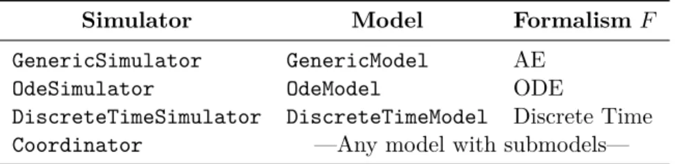
In this thesis, we follow the definition of a model introduced in (Defontaine, 2006): Definition 2.1 (Formalization of a model). A model M is a tuple denoted M (F, I, O, E, P) where I, O and E denote the input, output and state3variable sets, P denotes the parameter set of the model, and F is the formalism in which the model is described, which implicitly includes the definition of the corresponding output, transition or derivatives functions, when necessary.
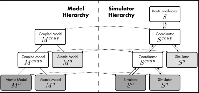
To account for models that represent a system as a set of components and their interac-tions (system specification level 4), we will complement the definition above with the formalization of two kind of models: atomic and coupled.
Definition 2.2 (Atomic and coupled models). An atomic model Ma is a model exactly as described in definition 2.1, whose dynamics are explained without any sub-components. A coupled model Mc(F, I, O, E, P, {Mi}) is a model composed of a set of components ({Mi}), i.e.
sub-models, which can be either atomic or coupled as well.
These definitions and their enclosed elements will be used and referenced throughout this manuscript, specially during the presentation of the contribution to formalism and multi-resolution modeling in chapters 3 and 4.
2.2.3 Simulation
According to the diagram of the modeling and simulation framework illustrated previously in fig. 2.3, when the system has been described, resulting in a complete model, an analysis should be performed in order to better understand the effect of the model parameters. However, these analyses use mostly the calculated outputs of the model, which are only known after a simulation. For this reason, it is more practical to explain the simulation process at this point.
2.2. General modeling and simulation framework 15
Figure 2.5– Mapping between experiment and simulation.
Simulations and models present a parallelism between the real model and experimentation, as illustrated in fig. 2.5. Accordingly, the term in silico is often used to refer to an experiment based on a computer simulation, in the same way the terms in vivo and in vitro experimentation are used in biology or physiology to refer to experiments performed in living organisms and isolated from their natural biological environment. In general, a simulation is the process that interprets the model definition to generate its output. This means that the simulation process must know the trajectories for each of its input variables, the values of each parameter, the initial values of internal states, and the specific definitions of each function according to the model formalism.
The simulation process tackles two distinct problems: i) the interpretation of the model specification under its formalism F , and ii) the simultaneous simulation of all the sub-systems defined within the model, when the model is composed of several components, as explained in the last level of system specification.The first problem is relevant to the formalism definition; along with the set of rules, relations and equations defined by a formalism, there is a set of devices or algorithms that permit to calculate the model dynamics. Therefore, the simulation process must use the corresponding algorithms to calculate the evolution of the model variables over time. For example, a model based on ordinary differential equations are simulated using a family of numerical integration methods that have been developed to provide a given accuracy (i.e. Euler method, the trapezoidal rule, or the Runge-Kutta methods). Hence, a simulator for models defined as a set of differential equations uses numerical methods specifically adapted to this particular formalism. In this example, it was mentioned that the solution to the model equations depend on a given accuracy. Indeed, the process of simulation is often an approximation that depends on an additional set of parameters, the simulation parameters, which affect the method that solves the dynamics of the model.
Continuing with the notation introduced in definitions 2.1 and 2.2, in this thesis we will consider the following formalization:
Definition 2.3 (Formalization of simulator and simulation). A simulator is represented by a process Sh(Mh, PS, F ) that calculates the evolution of a model Mh defined with formalism
16 Chapter 2. Modeling and Simulation
PS = [Psim, I, E0, P ] is a vector that defines the values for the simulation parameters (Psim), input
trajectories (I), initial conditions (E0) and the parameter (P ) of the model. A simulation, i.e
the execution of the process S, produces the outputs of the model, denoted O = Sh(Mh, P S, F ).
2.2.3.1 Multi-formalism simulation
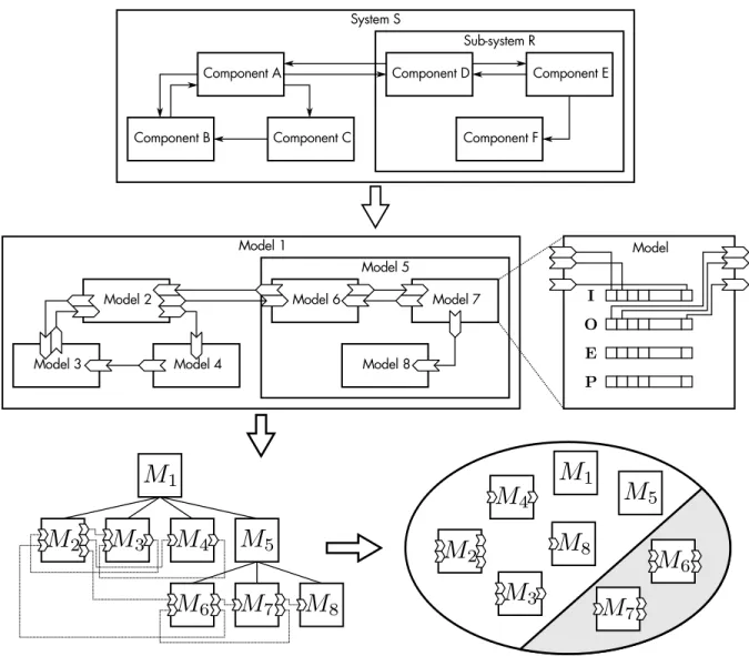
One of the major challenges concerning the simulation of complex models, usually defined at level 4 (coupled models Mcoup), arises when the model components (its atomic or coupled sub-models) are defined with different mathematical formalisms. The modeling of systems with different formalisms is termed multi-formalism modeling.
From the extensive studies of (De Lara et al., 2002; Vangheluwe, 2001; Zeigler et al., 2000), two main multi-formalism approaches have emerged: formalism transformation and co-simulation. An additional alternative, the meta-formalism approach, is often mentioned in the literature (Quesnel et al., 2009; Vangheluwe, 2000), but this case can be considered as a formalism transformation technique.
Formalism transformation: Based on the existence of morphisms between formalisms, this approach proposes that each component of the system must be transformed to a single formalism FU, for which a simulator is available. The formalism transformation approach has been one of
the cornerstones of (Zeigler et al., 2000), who defined a universal formalism, the Discrete Event System Specification (DEVS), that permits the coupling of differential equations with discrete-time and event systems. Other candidates include the hybrid differential algebraic equations (hybrid DAE, Vangheluwe, 2000) or the heterogeneous flow system specification (HFSS, Barros, 2003). Vangheluwe developed further this approach, whose contributions are summarized in the formalism transformation graph (FTG, cf. fig. 4.1): an exhaustive compilation of formalisms and their possible transformations to either DEVS or to difference equations.
The advantage of the formalism transformation approach is the fact that it only needs one simulator. More importantly, the usage of a common formalism does not require the definition of a particular coupling interface between models. However, this method lacks in practicality because it is difficult to design morphisms between formalisms and a transformed model is more difficult to interpret (Defontaine et al., 2004).
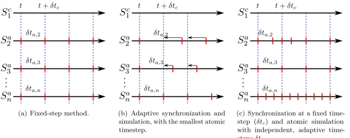
Co-simulation Based on the existence of formalism-specific simulators, this approach suggests that a system can be solved with several coordinated simulators. Avoiding the cumbersome and time-consuming task of formalism transformation, the co-simulation approach proposes that each model shall maintain its original formalism, and each model will be associated with a simulator specialized in this formalism. Consequently, each model is simulated in an independent, distributed fashion, yet the co-simulation must perform a precise inter-component coupling of input and output variables. However, this coupling of input and output variables in the trajectory level is not a straightforward task. Component coupling must contemplate two cases: i) when two connected models are simulated with a different temporal scale, and ii) when the outputs of a
2.2. General modeling and simulation framework 17
Figure 2.6– Formalism Transformation Graph (FTG), introduced by (Vangheluwe, 2001): solid lines represent an existing morphism that transforms one formalism to another. Gray dashed lines indicate the availability of a simulator for a formalism.
model cannot be directly set as an input of another model because they are expressed in different spatial references or even different mathematical structures. Nevertheless, the co-simulation approach is specially interesting because each model maintains its description, which permits the construction of complex models as a combination of the modeling efforts of different research fields. This combination aspect is interesting when applied to physiological modeling problems, in particular for multi-factorial physiological systems, where the dynamics of the system can only be explained if one considers its internal sub-systems and their intricate interactions.
Presently, multi-formalism simulation with a co-simulation approach is a field still in open research. The management of model coupling has been studied from a temporal-synchronization viewpoint (Hernández et al., 2009) and applied in several multi-factorial physiology appli-cations (Defontaine et al., 2004; Le Rolle et al., 2011; Thomas et al., 2008). From the viewpoint of component coupling, (Hernández et al., 2011) considers that the input/output pairing must be studied with an appropriate parameter analysis, e.g. a sensitivity analysis, in order to determine which variables should be considered in this coupling, and to evaluate the impact of such model integration. The modeling contribution of this work can be placed in this domain and it will be explained in detail in chapter 3.
2.2.4 Parameter analysis
As formalized in definition 2.3, the output of the model M are calculated through a simu-lation S and they depend on the value of the parameters (P ) that have been identified during
18 Chapter 2. Modeling and Simulation
the system description. Parameters are interesting to modelers and experimenters because, like the model itself, they represent a simplification of a particular element of the real world system. The next logical step of the modeling and simulation process would be to assign meaningful parameter values to the model. This enterprise can be as easy as observing the system and taking measures of some of its observable elements (e.g. measuring length, weight, volume, pressure, etc.). However, parameters are often impossible to observe or difficult to measure accurately; there is always an error associated with the parameter value. Moreover, model parameters may also represent an abstract object which is not physically measurable. Therefore, it is extremely important to acquire knowledge on the relation between the parameters and the outputs of the model.
Parameter analysis is the process that provides insight into the relation between parameters and outputs. It can consist in deductions from the mathematical equations that define the model. Yet, some relations are not evident and can be hidden within the complexity and interaction of different internal structures. Parameter analysis encompasses two different activities: i) the characterization of the effect of a parameter on the model dynamics, particularly its outputs, and ii) the identification or estimation of meaningful parameter values to the model. These two activities are conceptually independent, yet they are related since they can benefit from the information obtained from each other.
The effect of the system parameters, or more specifically the effect of a change of a parameter over the outputs can be identified when the equations of the model are simple enough to either deduce this or identify some of its properties. For instance, it is important to determine if the model is time-invariant, i.e. when the output of a system does not change with time, or if it is a linear model, i.e. when the output function satisfies the property of superposition (Karniel et al., 1999). Unfortunately, these properties are not easy to verify when the model comprises complex sub-systems and relations, when the model formalism does not admit this analysis, or when the parameters are numerous and highly interconnected. Nevertheless, in this case we will still be interested in the understanding on the effect that changes of the model parameters or inputs have over the model outputs. Keeping with definitions 2.1 and 2.3, this analysis attempts to comprehend∂O/∂Pand ∂O/∂I. These questions can be addressed with sensitivity analysis, the
study of how the alterations of the output of a mathematical model can be apportioned to the alterations in the model inputs or parameters. A review of this field and its related techniques will be presented later in section 4.2.
The second activity included in parameter analysis consists in finding the most adapted set of parameter values that can reproduce a set of experimental data. This process can be formalized as follows: From the perspective of the real system, let Oobs stand for an experimental
observation of the output of the system under certain conditions. Likewise, in the abstraction of the model and simulation, let Osim denote the simulated observation of the same output of
a model M , as formalized in definition 2.3, when simulated using the same conditions. The parameter estimation process consists in the exploration of the parameter space P in order to minimize a function of distance between the model predictions Osim and the experimental data
2.2. General modeling and simulation framework 19
Figure 2.7–Validation and verification schemes, according to (Vangheluwe, 2001).
Oobs. In other words, the parameter estimation aims to find the optimal parameter values Popt
defined as:
Popt= argmin P ∈P
g�(Osim(P ), Oobs)
subject to h(Osim(P )) ,
(2.1)
where g� is an error function and h is a generalization for a constraint function that indicates if
P is a feasible solution.
The difficulty of parameter estimation resides in three aspects: i) the definition of the observable variables and their corresponding simulated outputs, ii) the definition of the error function g�, and iii) the choice of the optimization method that solves eq. (2.1). A summary of
the available approaches to the definition and selection of the two last elements will be presented in section 4.3.
2.2.5 Validation
Finally, the last stage in the modeling and simulation framework is the validation analysis. This phase, however, is not necessarily the final step of the framework because it can be performed as soon as the system has been specified or described, and the validation results can eventually lead the investigator to restart the whole process.
The validation of the modeling process can occur at different levels, depending on the concept of validity used and which elements of the framework are being compared. Additionally, the definition of validation is different among the modeling and simulation literature. In this section, a merged definition of the existing validation concepts will be presented.
Following the identification presented in (Vangheluwe, 2001), there are four different validation schemes, summarized in fig. 2.7: structural validation, conceptual validation, behavioral validation and simulation verification:
– Behavioral validation is the evaluation of the simulated model behavior with respect to the system observations. This activity is a synonym to the term replicative validity of (Zeigler
20 Chapter 2. Modeling and Simulation
et al., 2000), which can only be affirmed when the experimental data and model output agree within an acceptable tolerance.
– Structural validation is the evaluation of the structure of the model with respect to the structure observed in the system. This validation encompasses two distinct concepts for Zeigler et al.: structural and predictive validity. Structural validity refers to an agreement between the state of the system and the model, which requires the observation or inference of this internal information; a difficult task for the system, but potentially easy for the model. A predictive validity is achieved when the model can generate outputs for cases where the system has not been directly observed.
– Conceptual validation is the relation between the system and the model in a conceptual level (not the simulation); it evaluates the realism of the model description with respect to the system and the experimental frame.
– Verification refers to the consistency between the model description and the interpretation provided by the simulator. Since simulators are not designed for a particular model, but to a family of models in a certain formalism, the verification, or simulator correctness is related with the question of how faithfully a simulation correctly generates the model outputs. Verification also refers to the analysis of the computer program that represents the model; i.e. the evaluation to ensure that the model implementation is correct and does not contain errors introduced by the modeler or programmer.
Although the experimental frame is briefly mentioned in the validation schemes, it is very pertinent during the validation phase. All schemes presented below are to be considered in the context of the experimental frame, in particular the behavioral and structural validation. In consequence, a model taken away from its experimental frame cannot be considered valid or invalid. Moreover, the results of the validation can reshape the experimental frame: when the model does not show replicative validity in some cases can help determine scenarios of the experimental frame that are more complicated than expected. Conversely, a model that shows good predictive validity can enlarge the experimental frame and the potential applications of the model.
While the activities presented below help categorize the validation process, it does not mention the available techniques to reach these validity relations. An extensive description of these techniques are presented in (Balci, 1994, 2010), which range from informal and manual approaches, to dynamic and advanced testing approaches. The detailed description of these approaches falls out of the scope of this work. However, it is worth mentioning that the sensitivity analysis and parameter identification processes presented in section 4.2 are the main tools that help identify some validity issues of the model.
2.3
Modeling and simulation in physiology
The concepts and definitions described in the previous sections are completely generic and are thus obviously applicable to biological or physiological systems. Indeed, the central role