HAL Id: hal-00450794
https://hal.archives-ouvertes.fr/hal-00450794v3
Submitted on 9 Feb 2010
HAL is a multi-disciplinary open access
archive for the deposit and dissemination of sci-entific research documents, whether they are pub-lished or not. The documents may come from teaching and research institutions in France or abroad, or from public or private research centers.
L’archive ouverte pluridisciplinaire HAL, est destinée au dépôt et à la diffusion de documents scientifiques de niveau recherche, publiés ou non, émanant des établissements d’enseignement et de recherche français ou étrangers, des laboratoires publics ou privés.
through dipole coupling
Gabriel Turinici, Herschel Rabitz
To cite this version:
Gabriel Turinici, Herschel Rabitz. Multi-polarization quantum control of rotational motion through dipole coupling. Journal of Physics A: Mathematical and Theoretical, IOP Publishing, 2010, 43 (10), pp.105303. �hal-00450794v3�
motion through dipole coupling
Gabriel Turinici
E-mail: [email protected]
CEREMADE, Universit´e Paris Dauphine, Place du Marechal De Lattre De Tassigny, 75775 PARIS Cedex 16, France
Herschel Rabitz
E-mail: [email protected]
Department of Chemistry, Princeton University, Princeton, NJ 08544-1009, USA
Abstract. In this work we analyze the quantum controllability of rotational motion under the influence of an external laser field coupled through a permanent dipole moment. The analysis takes into consideration up to three polarization fields, but we also discuss the consequences for working with fewer polarized fields.
1. Introduction
The manipulation of quantum phenomena is receiving increasing attention with laboratory demonstrations, including for control of rotational motion [1, 2, 3, 4, 5, 6]. A fundamental issue underlying such experiments is a basic assessment of the possibility of attaining full control in any particular physical circumstance. An assessment of this type concerns the controllability of quantum systems, and studies exist [7, 8, 9, 10, 11] based on the spectrum of the system field free Hamiltonian along with the coupling interaction to the control field. However, the treatment when the spectrum has degeneracies remains incomplete with the existing approaches either attempting to lift the degeneracy [8] or considering special coupling operators [10]. In particular, neither treatment permits the fundamental analysis of controllability of pure molecular rotational motion. This work addresses this situation in the context of dipole coupling and obtains positive controllability results. In addition, the analysis takes into consideration multi-polarization fields. This paper is relevant to other (non)-sudden alignment / orientation works [12, 13, 14, 15] and can also be seen as a step towards extending the treatment to a general assessment of controllability of vibration-rotation states. An additional related topic is rotational control through non-resonant polarization interactions [16], which will be treated in a separate work.
2. Physical picture
Consider a linear rigid molecule described by the Hamiltonian H = B ˆJ2 where B is the rotational constant and ˆJ the is the angular momentum operator. The molecule’s rotational motion is subject to control through external interactions with an electric field −→ǫ(t), which couples to the molecule through the dipole operator −→d. The time dependent Schr¨odinger equation is
i~∂
∂t|ψ(θ, φ, t)i = (B ˆJ
2−−→ǫ(t) ·−→d) |ψ(θ, φ, t)i (1)
|ψ(0)i = |ψ0i , (2)
where θ and φ are the standard polar coordinates. We consider that the external field −→
ǫ(t) is multi-polarized i.e. any of its x, y, z components can be tuned independently as a function of time. See Section 4 for discussion of other situations.
For convenience we express the problem in spherical harmonics |Ym
J i, J ≥ 0 and
−J ≤ m ≤ J as the eigenbasis of the operator H = B ˆJ2such that B ˆJ2|Ym
J i = EJ|YJmi,
EJ = BJ(J + 1). The difference between two consecutive eigenvalues EJ+1 − EJ =
2B(J + 1) increases with J. Thus, beyond some threshold value of J depending on the control field characteristics, this gap will lie outside of the available frequency range of the field in any practical situation. As such, we will truncate the set of spherical harmonics |YM
J i at a suitable value Jmax and consider control over the domain of states
Remark 1 The truncation is supported here by the convenient spectral properties of the operator B ˆJ2 having only discrete eigenvalues which become increasingly sparse as the energy increases. In particular, no accumulation of the discrete spectrum towards a continuous spectral region is present. However, the impact of truncation in other contexts is not always transparent for assessing controllability. For instance, any finite dimensional truncation of the linearly driven harmonic oscillator [10, 17] is controllable, but the infinite dimensional system is not. In that situation the gaps between consecutive eigenvalues are all equal, and a sufficiently long external control pulse can lead to excitation of states indefinitely high in the spectrum.
Remark 2 A circumstance may occur when the wavefunction is stimulated to populate eigenfunctions of increasing energy and even go to dissociation [6]; the field frequency increases indefinitely in order to address this increasing energy gap between two consecutive eigenvalues. This situation is beyond the treatment here that only considers bound states remaining within a given energy range.
The dipole interaction −→ǫ(t) ·−→d may be expressed as ǫx(t)x + ǫy(t)y + ǫz(t)z in
terms of space fixed cartesian coordinates −→x, −→y and −→z , where each of the components ǫx(t), ǫy(t), ǫz(t) of the field can be tuned independently.
The J = 1 spherical harmonics Y1±1 = ∓1 2 r 3 2π x± iy r , Y 0 1 = 1 2 r 3 π z r, (3)
may be written in the rotated frame −→x√+i−→y 2 ,
− →x−i−→y
√
2 and −→z. Choosing this latter frame
we obtain −→ǫ(t) · −→d = ǫ0(t)d10Y10 + ǫ+1(t)d11Y11 + ǫ−1(t)d1−1Y1−1. For convenience the
components d10, d11, d1−1 of −→d are assumed to be all nonzero and will be rescaled to 1
(this is equivalent to rescaling the components ǫ0, ǫ+1 and ǫ−1 of
−→
ǫ(t)) so that we obtain −→
ǫ(t) ·−→d = ǫ0(t)Y10+ ǫ+1(t)Y11+ ǫ−1(t)Y1−1.
Let Dk be the matrix of the spherical harmonic operator Y1k (k = −1, 0, 1). The
associated matrix elements may be written as [18]: (Dk)(Jm),(J′m′)= hYJm|Yk 1 |Y m′ J′ i = Z (YJm)∗(θ, φ)Y k 1 (θ, φ)Y m′ J′ (θ, φ) sin(θ)dθdφ = r 3(2J + 1)(2J′+ 1) 4π Ã J 1 J′ 0 0 0 ! Ã J 1 J′ m k m′ ! . (4)
where the real constants à J 1 J′ 0 0 0 ! and à J 1 J′ m k m′ !
are Wigner 3J-symbols (see [19] Chapter 2 for formulas and details). The non-zero elements satisfy the criteria m+ k + m′ = 0 and |J − J′| = 1. Thus, the only non-zero entries of the matrix D
−1
are between states |Ym
J i and |YJ+1−m+1i; we will say that D−1 couples states |YJmi and
|YJ+1−m+1i; similarly D0 only couples |YJmi and |YJ+1−mi and D1 only couples |YJmi and
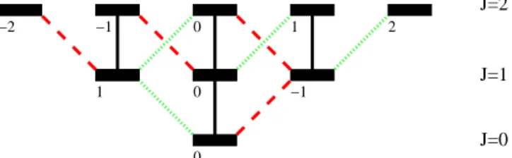
J=2 J=1 J=0 0 0 0 1 1 2 −2 −1 −1
Figure 1. The three matrices Dk, k = −1, 0, 1 coupling the eigenstates are each represented by a different line style (dotted, solid and dashed) for Jmax = 2. On the J-th line from bottom, the states are from left to right in order |Ym=−J
J i , ..., |Y m=J J i for even values of J and |Ym=J
J i , ..., |Y m=−J
J i for odd values of J. The m quantum number labelings are indicated in the figure. The coupling pattern above continues in a similar fashion for Jmax>2.
Denoting by Ψ(t) the coefficients of ψ(θ, φ, t) with respect to the spherical harmonic basis, the Schr¨odinger equation in matrix form is
(
i∂t∂Ψ(t) = (E − ǫ0(t)D0− ǫ−1(t)D−1− ǫ1(t)D1)Ψ(t)
Ψ(t = 0) = Ψ0.
(5) where E is the diagonal matrix with entries EJ for all dual indexes Jm with −J ≤ m ≤ J
and J ≤ Jmax.
3. Controllability assessment with three independently polarized field components
We desire to determine whether the system is controllable over all of its J and m states up to Jmax provided that all of the control field components ǫk(t) k = −1, 0, 1 can be
chosen independently. Intuitive arguments were given in [15] (pages 437-438) on why the answer to this question should be positive for all truncation values Jmax. The material
below provides a rigorous grounding for this claim.
Theorem 1 Let Jmax ≥ 1 and denote N = (Jmax + 1)2. Let E, Dk, k = −1, 0, 1 be
N × N matrices indexed by Jm with J = 0, ..., Jmax, |m| ≤ J where:
EJ m;J′m′ = δJ J′δmm′EJ (6) (D0)J m,J′m′ 6= 0 ⇔ |J − J′| = 1, m + m′ = 0 (7) (D1)J m,J′m′ 6= 0 ⇔ |J − J′| = 1, m + m′+ 1 = 0 (8) (D−1)J m,J′m′ 6= 0 ⇔ |J − J′| = 1, m + m′− 1 = 0. (9)
and recall that
EJ = J(J + 1). (10)
Then the system described by E, D−1, D0, D1 is controllable.
Proof. In view of the criterion in [7] we have to prove that the Lie algebra L generated by iE and iDk k= −1, 0, 1 is u(N ).
We label by e(ab) the N × N matrix whose entry at row a and column b is 1
and all others are zero and denote V(ab) = i¡e(ab)+ e(ba)¢, S(ab) = ¡e(ab)− e(ba)¢ and
∆a = i¡e(aa)− e(a+1;a+1)¢. Note that S(ab), V(ab), (a < b, a, b = 1, N ) and ∆a
(a = 1, ..., N − 1) form a basis for su(N ). We index by ξ ∈ Ξ (of cardinality K) the entries ξ = (ab) , a < b such that at least one matrix Dk has a non-zero entry
(Dk)ξ=(ab) 6= 0 and denote by ξ† the pair (ba).
We will index the matrices E and Dkwith a, b running from 1 to N : E = (E)Na,b=1,
Dk = (Dk)Na,b=1, k = −1, 0, 1 where we choose the order for (Jm) : (00) corresponds
to a = 1, (11) corresponds to a = 2, (10) to a = 3, (1 − 1) to a = 4, then (2−2), (2−1), (20), (21), (22), ... etc (see Fig 1). Note that (Jm) traverses from m = −J to m = J for even values of J and from m = J down to m = −J for odd values of J. For instance E44= E(1−1),(1−1) = 2. When there is no ambiguity we will use interchangeably
(1 −1) or 4, etc.
For k = −1, 0, 1 and ℓ ≥ 1 we compute adℓ
iEiDk = [iE, ..., [iE, iDk]...] =
(iℓ+1ωℓ
ab(Dk)ab)Na,b=1 (ωab = Eaa − Ebb) with the iterative commutators taken ℓ times.
Consider the basis vkJ = X
ξ=(ab),ωξ=EJ +1−EJ;a<b;(Dk)ξ6=0
(Dk)ξeξ , vJk† = X
ξ=(ab),ωξ=EJ +1−EJ;a<b;(Dk)ξ6=0
(Dk)∗ξ†eξ† ; J = 0, ..., Jmax (11) and note that adℓ
iEiDk =Pk,Jiℓ+1ωξℓvkJ + iℓ+1(−1)ℓ(ωξ)ℓvJk†. We obtain as in [20] that,
since ωξ are all different, adℓiEiDk generates any vector in the linear space
V ect X
ξ=(ab),ωξ=EJ +1−EJ;a<b;(Dk)ξ6=0
(Dk)ξSξ , X
ξ=(ab),ωξ=EJ +1−EJ;a<b;(Dk)ξ6=0
(Dk)∗ξ†Vξ† ; J = 0, ..., Jmax . (12) In particular, X
ξ=(ab),ωξ=EJ +1−EJ;a<b;(Dk)ξ6=0
(Dk)ξSξ and X
ξ=(ab),ωξ=EJ +1−EJ;a<b;(Dk)ξ6=0
(Dk)∗ξ†Vξ†
will belong to L, J = 0, ..., Jmax.
For J = 0 we obtain S(a=(00),b=(10)), S(a=(00),b=(1−1)), S(a=(00),b=(11)) ∈ L and the same
for V(a=(00),b=(1m)), m = −1, 0, 1. We recall now the relations
for a 6= b 6= c 6= a : [S(ab), S(bc)] = S(ac), [S(ab), V(bc)] = V(ac),
for a, b, a′, b′ all different : [S(ab), S(a′b′)] = 0, [S(ab), V(a′b′)] = 0,
and note that the commutators S(a=(00),b), X ξ=(b′c′),ω ξ=E2−E1;b′<c′;(Dk)ξ6=0 (Dk)ξSξ
contain only one term (Dk)(bc)S(ac) where c = (2c2) is the (level J = 2) state coupled
with state b = (1b2) (level J = 1) through the same matrix Dk that also couples
the state a (level J = 0) and b: (Dk)(ab) 6= 0 6= (Dk)(bc). Thus S(ac) ∈ L and, by
using the commutator of S(ab) and S(ac), we obtain that S(bc) is in L as well for any
ξ = (b = (1m), c = (2m′)) such that (Dk)ξ 6= 0 for some k = −1, 0, 1. It remains now
to iterate the above treatment for all levels J = 2, ..., Jmax to obtain that all Sξ and Vξ
coupled by some matrix k : (Dk)ξ 6= 0 are in L. We note that the graph [8, 9, 11] of
the system is connected and conclude that L = u(N ). ¤
Remark 3 The same conclusion as that of Thm. 1 holds if one replaces (10) by the more general condition
EJ+1− EJ 6= EJ′+1− EJ′,∀J 6= J′. (14)
Theorem 2 Consider a finite dimensional system where a set of states, indexed as
a= (Jm) with J = 0, ..., Jmax, m = 1, ..., mmax
J , mmax0 = 1, are such that
EJ m;J′m′ = δJ J′δmm′EJ (15)
EJ+1− EJ 6= EJ′+1− EJ′,∀J 6= J′. (16)
We also introduce the set of K external interactions with corresponding matrices Dk,
k = 1, ..., K where Dk only couples states (Jm) and (J′m′) such that |J − J′| = 1 and only one non-zero coupling exists for any (Jm):
(Dk)(Jm),(J′m′)6= 0 ⇒ |J − J′| = 1 (17) (Dk)(Jm),(J′m′)6= 0, (Dk)(Jm),(J′′m′′) 6= 0, J ≤ J′ ≤ J′′ ⇒ J′ = J′′, m′ = m′′(18)
We also suppose that the graph [8, 9, 11] of the system is connected. Then the system described by EJ, Dk (J = 0, ..., Jmax, k = 1, ..., K) is controllable.
Proof. Under the assumptions above, the proof follows exactly the same path as the one of the Thm. 1.¤
Remark 4 The transition energy condition in Eqns. (14) and (16) is consistent with the rotation of a linear rigid molecule. In addition the further flexibility encompasses broader circumstances including the possibility of hindered rotation of a molecule residing in a trapped nanoscale environment. Moreover, when hypothesis (15) is not satisfied because the system is not degenerate previous results apply [8, 9, 10, 11].
Remark 5 The results above can be extended to the case of a symmetric top molecule; in such a circumstance [18] the energy levels are described by three quantum numbers
EJ Km with |m| ≤ J, |K| ≤ J and
EJ Km= C1J(J + 1) + C2K2, (19)
for some constants C1 and C2. If the initial state is in the ground state, or any other state with K = 0 the coupling operators have the same structure as in Thm. 1 and thus any linear combination of eigenstates with quantum numbers J, K = 0, m can be reached (same result directly applies). A more detailed analysis of symmetric top molecules will be presented in a future work.
4. Controllability for a locked combination of lasers
We consider here whether the positive result above is still true when ǫk(t), k = −1, 0, 1
are not chosen independently but with a locked linear dependence through coefficients αk such that
−→
ǫ(t) ·−→d = ǫ(t){α−1Y1−1+ α0Y10+ α1Y11}. Note that there may exist cases
that are not controllable for any given linear combination. One such example is :
E = 0 0 0 0 0 2 0 0 0 0 2 0 0 0 0 2 , −−→e(t) ·−→d = ǫ(t)µ, µ = 0 α−1 α0 α1 α−1 0 0 0 α0 0 0 0 α1 0 0 0 . (20)
This system is such that for all αk(k = −1, 0, 1 ) the Lie algebra generated by iE and iµ
is u(2), thus the system is not controllable with one laser field. However, Thm. 1 shows that it will become controllable provided that the three components ǫk(t), k = −1, 0, 1
can be chosen independently.
The following result describes this situation further.
Theorem 3 Let A,B1,...,BK be elements of a finite dimensional Lie algebra L. For α =
(α1, ..., αK) ∈ RK we denote Lα as the Lie algebra generated by A and Bα =PKk=1αkBk. Define the maximal dimension of Lα
d1A,B1,...,BK = max
α∈RKdimR(Lα). (21)
Then with probability one with respect to α, dim(Lα) = d1
A,B1,...,BK.
Remark 6 This theorem states that for fixed A, B1, ..., BK all choices of α give a Lie algebra Lα of maximal dimension with the possible exception of at most a null measure set. This dimension d1
A,B1,...,BK is specific to the choice of coupling operators Bk but
can be easily computed by the property above. On the other hand, recall that [21] when
A,B1, ..., BK are r ×r skew-hermitian matrices the system is generically controllable i.e., we have d1
A,B1,...,BK = r
2 for generic A, B1, ..., BK.
Proof. Consider the (countable) collection Cα = {ζα
1 = A, ζ2α = B, ζ3α = [A, Bα], ζ4α =
A and Bα. Now take a subset {ζiα1, ..., ζ α ir} of C α; the vectors ζα i1, ..., ζ α ir are linearly independent when the Gram determinant is non-null. Note that the Gram determinant is an analytic function of α; hence one of the following alternatives is true: either this function is identically null for all α (which is the case e.g., for {ζα
3, ζ4α} ) or it is
non-null everywhere with the possible exception of a zero measure set. Since the number of subsets {ζα
i1, ..., ζ
α ir} of C
α is countable, we can construct F ⊂ RK whose complement
RK\ F is of zero measure such that if ζiα 1, ..., ζ
α
ir are linearly independent for one value of α ∈ RK then they are linearly independent for all α′ ∈ F. Denote by α⋆ some value
such that dimR(Lα⋆) = d1A,B
1,...,BK; then there exists a set such that {ζ
α⋆ i1 , ..., ζ α⋆ id1 A,B1,...,BK } are linearly independent implying that {ζα⋆
i1 , ..., ζ
α⋆
id1
M
} are linearly independent for any α ∈ F; thus dimR(Lα) ≥ d1A,B1,...,BK for all α ∈ F and the conclusion follows by the maximality of d1
A,B1,...,BK.
We invoked Remark 6 and performed numerical tests by computing the Lie algebra generated by iE and iDα = iP1k=−1αkDk. The theorem was verified and we obtained
for any fixed Jmaxand randomly chosen values of α that the dimensions of the Lie algebra
are the same. We also observed that the Lie algebra generated by iE and iP1
k=−1αkDk
always had dimension (N − 2)2 which leads to the conjecture that generically in α (see
Thm 3) the Lie algebra generated by iE and iP1
k=−1αkDk is isomorphic to u(N − 2).
Recall that by Thm. 1 when three independent control intensities are allowed then this Lie algebra is u(N ). We have as yet no theoretical explanation of why this appears to be true. This observation shows, nevertheless, the extent to which a locked set of laser intensities is sufficient to obtain specific attainable control targets.
5. Controllability with two lasers
We consider in this section the situation when two laser fields are used i.e. one can independently shape the intensity along two vectors −→α and −→β: −→ǫ(t) · −→d = ǫα(t){α−1Y1−1 + α0Y10 + α1Y11} + ǫβ(t){β−1Y1−1 + β0Y10 + β1Y11}. Examples of such
situations are shaping along −→x and −→z directions, −→x and −→y directions or any other two independent vectors.
Theorem 4 Let A,B1,...,BK be elements of a finite dimensional Lie algebra L. We denote for α = (α1, ..., αK) ∈ RK and β = (β1, ..., βK) ∈ RK by Lα,β the Lie algebra generated by A, Bα =PK
k=1αkBk and Bβ =PKk=1βkBk. Define the maximal dimension of Lα
d2A,B1,...,BK = max
α∈RKdimR(Lα,β). (22)
Then with probability one with respect to α, β, dim(Lα,β) = d2
A,B1,...,BK. Proof. The proof is similar to that of Thm.3. ¤
This theorem states that all choices of α, β give the maximal Lie algebra dimension dim(Lα,β) = d2A,B1,...,BK with the possible exception of at most a null measure set. We will analyze in the following two particular cases.
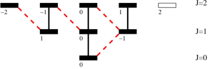
J=2 J=1 J=0 0 0 0 1 1 2 −2 −1 −1
Figure 2. The same conventions as in Fig. 1 are used except that we do not draw on the coupling by D−1. We note that the state |Ym=Jmax
Jmax i is not connected with the
others.
5.1. Field shaped in the −→z and −→x√+i−→y
2 directions
When the field is shaped in the −→z and −→x√+i−→y
2 directions we obtain, with the notation of
previous sections, that ǫ0(t) and ǫ1(t) are arbitrary and ǫ−1 is null. This is not a generic
case in the sense of Thm. 4 because the shaping directions are precisely related to the system structure. We note that since ǫ−1 = 0 the coupling realized by the operator D−1 (dotted in Fig. 1) disappears and the state |Ym=Jmax
Jmax i will not be reachable (see Fig. 2). This means that the population in state |Ym=Jmax
Jmax i cannot be changed by the two lasers and thus will be a conserved quantity.
Theorem 5 Consider the model of Thm.1 with ǫ−1 = 0. Let |ψIi and |ψFi be two states that have the same population in |Ym=Jmax
Jmax i i.e., |hψI, Y
m=Jmax
Jmax i|
2 = |hψ
F, YJm=Jmaxmaxi|2. Then |ψFi can be reached from |ψIi with controls ǫ0(t) and ǫ1(t).
Proof: The conclusion is a consequence of Thm. 2 for K = 2 and using all spherical harmonics |Ym
J i except |YJm=Jmaxmaxi. Thus we conclude that the Lie algebra has dimension N2 and by the independent system controllability criterion in [22, 23] we obtain the conclusion. ¤
A similar analysis applies when the field is shaped in the −→z and −→x√−i−→y
2 directions
with the modification that in this case the population of |Ym=−Jmax
Jmax i is conserved and the compatibility relation reads:
|hψI, YJmmax=−Jmaxi|
2 = |hψ
F, YJmmax=−Jmaxi|
2. (23)
5.2. Field shaped in the −→x√+i−→y 2 and
− →x−i−→y
√
2 directions
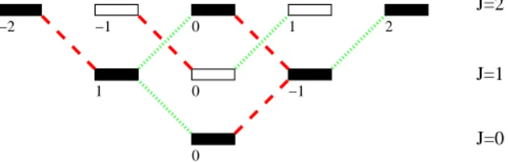
Using the same notation, now ǫ−1(t) and ǫ1(t) are arbitrary and ǫ0 is null. Thus, the
states are divided in two components cf. Fig. 3: X1 = {|Y00i , |Y1±1i , |Y2±2i , |Y20i , ...}
and X2 = {|Y10i , |Y2±1i , |Y3±2i , |Y30i , ...} with no coupling between the two components.
The conservation law reads X |Ym J i∈X1 |hψI, YJmi|2 = X |Ym J i∈X1 |hψF, YJmi|2. (24)
J=2 J=1 J=0 0 0 0 1 1 2 −2 −1 −1
Figure 3. The same conventions as in Fig. 1 are used except that we do not draw on the coupling by D0. We note that two connectivity sets appear: those connected with |Y0
0i (filled black rectangles) and those connected with |Y 0
1i (empty rectangles).
Theorem 6 Consider the model of the Thm.1 with ǫ−1 = 0. Let |ψIi and |ψFi be two states compatible in the sense of Eqn. (24). Then |ψFi can be reached from |ψIi with controls ǫ−1(t) and ǫ1(t).
Proof: The proof follows that of Thm. 2 except that the system has now two independent graphs instead of one, both satisfying the hypothesis of the theorem. The same computation alows one to generate the full Lie algebra for X1 (using that for
the graph containing the states X1 we have mmax0 = 1). Next, one works with the
second graph and constructs its associated algebra. The conclusion is obtained by the independent system controllability criterion in [22, 23]. ¤
6. Conclusions
This paper discussed the controllability properties of molecular rotation with multi-polarization fields that act through a permanent dipole moment. A first conclusion is that the degeneracy of the energy levels brings no additional restriction on the controllability. Positive results are found for the controllability of an arbitrary number of rotation eigenstates. We also discussed the situation of a symmetric top molecule when the magnetic quantum number m is zero.
The dependence of the controllability result on the the coupling operators is not surprising; however as in [9] the numeric values of the entries of the coupling matrices are not important as soon as they are non-null. Thus, we can say that the controllability depends only on the ”selection rules” i.e. on the fact that two states may, or may not, have a non-vanishing coupling through one of the external (laser) interactions.
The situation with one and two polarized fields was also examined based on the generic dimension of the Lie algebra. For the particular situations where the field is shaped in any combination of two of the three directions −→z, −→x√+i−→y
2 and
− →x−i−→y
√
2 we
showed that the system is still controllable provided that the target is consistent with the selection rules. Breaking those symmetries would require a third independently shaped pulse.
The specific situation with two fields depends on which dual polarization components are available: if one can shape the polarization in the −→z and −→x√+i−→y
directions everything can be controlled except the population of the state |Ym=Jmax
Jmax i (respectively |Ym=−Jmax
Jmax i for the −
→z and −→x√−i−→y
2 directions). If on the contrary the
field can be shaped in the −→x√+i−→y 2 and
− →x−i−→y
√
2 directions, then the initial and target
state have to be compatible in the sense of the selection rules. We note that in both cases with two polarization field components (in the list above) one only has a single compatibility constraint to satisfy. This is to be contrasted with the situation when only one polarization component is available : in this case there are many constraints on the target state (e.g., when only ǫ0is available the selection rules impose 2Jmax+1 constraints
because m is conserved). In summary, the most substantial increase in controllability (based on our analysis of these particular cases and on the general controllability result) is witnessed when replacing a linear polarized field by a field independently shaped in two directions.
Finally, it is important to place this work in the larger context of molecular, and more generally quantum system, controllability. A pertinent issue is whether any randomly chosen Hamiltonian (i.e., a particular physical system drawn from the stockroom) is likely to be controllable. Building on theoretical results [21], recent numerical work [24] argued that virtually any Hamiltonian-coupling operator (i.e., the dipole) expressed in the eigenbasis of the field free Hamiltonian H0 will generate a
connected graph (e.g., as in Fig. 1 versus that in Fig. 2). Although this statement is short of establishing controllability, it is a necessary criteria. Furthermore, to arrange a special relationship amongst the Hamiltonian’s matrix elements in order to violate controllability is a demand whose solution lies in the null space of all Hamiltonians [8, 11]. In particular we proved in this paper that this null space does not contain the degenerate Hamiltonian for rotational motion. Thus, although uncontrollable Hamiltonians can be designed, the chance of finding one in the laboratory is very small. This conclusion provides the basis to expect that suitable control fields will virtually always exist yielding high quality results.
Acknowledgments
G.T. acknowledges support from the French ANR C-QUID project, INRIA Rocquencourt (MicMac and OMQS projects) and PICS-NSF program ”Manipulation and identification of quantum phenomena”. H.R. acknowledges support from the DoE. References
[1] Richard S. Judson and H. Rabitz. Teaching lasers to control molecules. Phys. Rev. Lett, 68:1500, 1992.
[2] A. Assion, T. Baumert, M. Bergt, T. Brixner, B. Kiefer, V. Seyfried, M. Strehle, and G. Gerber. Control of chemical reactions by feedback-optimized phase-shaped femtosecond laser pulses.
Science, 282:919–922, 1998.
[3] T.C. Weinacht, J. Ahn, and P.H. Bucksbaum. Controlling the shape of a quantum wavefunction.
[4] R. Bartels, S. Backus, E. Zeek, L. Misoguti, G. Vdovin, I.P. Christov, M.M. Murnane, and H.C. Kapteyn. Shaped-pulse optimization of coherent emission of high-harmonic soft x-rays. Nature, 406:164–166, 2000.
[5] R. J. Levis, G.M. Menkir, and H. Rabitz. Selective bond dissociation and rearrangement with optimally tailored, strong-field laser pulses. Science, 292:709–713, 2001.
[6] D. M. Villeneuve, S. A. Aseyev, P. Dietrich, M. Spanner, M. Yu. Ivanov, and P. B. Corkum. Forced molecular rotation in an optical centrifuge. Phys. Rev. Lett., 85(3):542–545, Jul 2000.
[7] V. Ramakrishna, M.V. Salapaka, M. Dahleh, H. Rabitz, and A. Peirce. Controllability of molecular systems. Phys. Rev. A, 51 (2):960–966, 1995.
[8] Gabriel Turinici and Herschel Rabitz. Quantum wave function controllability. Chem. Phys., 267:1–9, 2001.
[9] Gabriel Turinici and Herschel Rabitz. Wavefunction controllability in quantum systems. J. Phys.A., 36:2565–2576, 2003.
[10] S. G. Schirmer, H. Fu, and A.I. Solomon. Complete controllability of quantum systems. Phys.
Rev. A, 63:063410, 2001.
[11] C. Altafini. Controllability of quantum mechanical systems by root space decomposition of su(N).
J.Math.Phys., 43(5):2051–2062, 2002.
[12] Henrik Stapelfeldt and Tamar Seideman. Colloquium: Aligning molecules with strong laser pulses.
Reviews of Modern Physics, 75(2):543, 2003.
[13] D. Sugny, A. Keller, O. Atabek, D. Daems, C. M. Dion, S. Gu´erin, and H. R. Jauslin. Reaching optimally oriented molecular states by laser kicks. Phys. Rev. A, 69(3):033402, Mar 2004. [14] A. Keller, C. M. Dion, and O. Atabek. Laser-induced molecular rotational dynamics: A
high-frequency Floquet approach. Phys. Rev. A, 61(2):023409, Jan 2000.
[15] R.S. Judson, K.K. Lehmann, H. Rabitz, and W. Warren. Optimal design of external fields for controlling molecular motion: application to rotation. J. Molec. Structure, 223:425–456, June 1990.
[16] R. S. Minns, R. Patel, J. R. R. Verlet, and H. H. Fielding. Optical control of the rotational angular momentum of a molecular Rydberg wave packet. Phys. Rev. Lett., 91(24):243601, Dec 2003. [17] Mazyar Mirrahimi and Pierre Rouchon. Controllability of quantum harmonic oscillators. IEEE
Trans. Automat. Control, 49(5):745–747, 2004.
[18] D.M. Brink and G.R. Satchler. Angular Momentum. Oxford University Press, 1994. [19] Richard Z. Zare. Angular Momentum. John Wiley & Sons, 1988.
[20] Gabriel Turinici and Herschel Rabitz. Optimally controlling the internal dynamics of a randomly orientated ensemble of molecules. Phys. Rev. A, 70:063412, 2004.
[21] Nik Weaver. On the universality of almost every quantum logic gate. Journal of Mathematical
Physics, 41(1):240–243, 2000.
[22] B. Li, G. Turinici, V. Ramakhrishna, and H. Rabitz. Optimal dynamic discrimination of similar molecules through quantum learning control. Journal of Physical Chemistry B, 106(33):8125– 8131, 2002.
[23] G. Turinici, V. Ramakhrishna, B. Li, and H. Rabitz. Optimal discrimination of multiple quantum systems: Controllability analysis. Journal of Physics A: Mathematical and General, 37:273–282, 2003.
[24] Rong Wu, Herschel Rabitz, Gabriel Turinici, and Ignacio Sola. Connectivity analysis of controlled quantum systems. Phys. Rev. A, 70(5):052507, Nov 2004.