Desalination of brackish groundwater in the United States : minimum energy requirements

Desalination of Brackish Groundwater in the United

States:

Minimum Energy Requirements

by

Yvana D. Ahdab

B.S., Johns Hopkins University (2015)

Submitted to the Department of Mechanical Engineering

in partial fulfillment of the requirements for the degree of

Master of Science in Mechanical Engineering

at the

MASSACHUSETTS INSTITUTE OF TECHNOLOGY

June 2017

@

Massachusetts Institute of Technology 2017. All rights reserved.

Author... ....

...

D....

...

Department of Mechanical Engineering

May 12, 2017

Certified by...

...

...

John H. Lienhard V

dul Latif Jameel Professor of Water

Thesis Supervisor

Accepted by...

JUN

21101

LIBRARIES

. . .. .

...

Rohan Abeyaratne

Chairman, Committee on Graduate Students

Desalination of Brackish Groundwater in the United

States:

Minimum Energy Requirements

by

Yvana D. Ahdab

B.S., Johns Hopkins University (2015)

Submitted to the Department of Mechanical Engineering

in partial fulfillment of the requirements for the degree of

Master of Science in Mechanical Engineering

at the

MASSACHUSETTS INSTITUTE OF TECHNOLOGY

June 2017

@

Massachusetts Institute of Technology 2017. All rights reserved.

Signature redacted

A uthor...

_...

_...

Department of Mechanical Engineering

May 12, 2017

Certified by

Signature redacted

John H. Lienhard V

ul Latif Jameel Professor of Water

Thesis Supervisor

Accepted by ...

JUN

2

1017

LIBRARIES

Signature redacted

Rohan Abeyaratne

Chairman, Committee on Graduate Students

Desalination of Brackish Groundwater in the United States:

Minimum Energy Requirements

by

Yvana D. Ahdab

Submitted to the Department of Mechanical Engineering on May 12, 2017, in partial fulfillment of the

requirements for the degree of

Master of Science in Mechanical Engineering

Abstract

Water scarcity around the globe has motivated rising interest in desalinating brack-ish groundwater to meet fresh water demand. Various organizations in the United States have collected more hydrological and chemical data from the growing num-ber of wells. Yet, only one national assessment of groundwater resource distribution and availability has been conducted in the United States since the 1960s, and no na-tional assessment has been conducted on the energy costs required to make brackish groundwater potable. Because the ionic composition of groundwater varies signifi-cantly from location to location, unlike seawater, conducting site-specific analyses of the resource across the U.S. is necessary. This thesis uses chemical and physical data from a U.S. Geological Survey dataset compiled in 2017, including samples from over

100,000 groundwater wells across the United States, to carry out a nationwide

investi-gation of brackish groundwater composition and minimum desalination energy costs. Beginning with a full Pitzer-Kim mixed electrolyte model, we develop a thermody-namic analysis of the least work of separation in order to compute the site-specific least work of separation required for groundwater desalination. Least work of separa-tion represents a baseline for specific energy consumpsepara-tion of real-world desalinasepara-tion systems. Then, we study the geographic distribution of least work of separation to determine areas with both low least work of separation and high water stress. These regions hold potential for desalination to decrease the disparity between high water demand and low water supply. We develop simplified equations for least work as a function of recovery ratio and the following parameters: total dissolved solids, specific conductance, ionic strength, and molality. Lastly, we examine the effects of ground-water composition on minimum energy costs, and the geographic distribution of total dissolved solids, well depth and major ions.

Thesis Supervisor: John H. Lienhard V Title: Abdul Latif Jameel Professor of Water

Acknowledgments

My deepest gratitude is extended to my advisor, Professor John Lienhard. His

guid-ance, technical expertise, and support have been invaluable. I would like to thank my former lab mate, Gregory P. Thiel, for his crucial contributions to this work. Acknowledgment is also given to my lab mates and friends in the Lienhard Research Group for valuable discussions and advice.

I would also like to thank the U.S. Geological Survey for providing the dataset necessary to carry out the analyses in this thesis and to the Center for Clean Water Energy at MIT and the King Fahd University of Petroleum and Minerals for funding the research reported in this thesis.

Finally, to my close friends (special shout-outs to the block of cheese club and the squad) and family, I am deeply grateful for your encouragement and confidence in me. Mom and dad, you in particular have felt my joy (and pain) throughout this process. I cannot express how appreciative I am today, and every day, to have your unwavering support.

Contents

1 Motivation and background 23

1.1 The water crisis in the United States . . . . 23

1.2 Water use in the United States . . . . 24

1.2.1 Water use from 1950 to 2010 . . . . 25

1.2.2 W ater use in 2010 . . . . 26

1.2.3 Water quality requirements based on water use . . . . 27

1.3 Desalination in the United States . . . . 29

1.4 Minimum energy requirements for brackish groundwater desalination to meet low salinity water demand in the United States . . . . 31

2 U.S. Geological Survey major-ions dataset 35 2.1 Coverage . . . . 35

2.2 Lim itations . . . . 36

3 Methodology 39 3.1 Derivation of least work of separation . . .. . . . 39

3.2 Calculations . . . . 42

3.2.1 Evaluation of activity coefficients for least work of separation using Pitzer mixed electrolyte model . . . . 42

3.2.2 Density, alkalinity, and correlation coefficient . . . . 47

4 Least work of separation 49 4.1 Geographic distribution . . . . 49

4.2 Correlation trends . . . . 54

4.2.1 Total dissolved solids . . . . 54

4.2.2 Specific conductance . . . . 56

4.2.3 M olality . . . . 58

4.2.4 Ionic strength . . . . 59

5 Chemical composition 63 5.1 M ajor ions . . . . 63

5.2 Effect of major ions on least work of separation . . . . 64

5.3 Geographic distribution of total dissolved solids, well depth, and major ions ... ... ... 67

5.3.1 Total dissolved solids and well depth . . . . 68

5.3.2 M ajor cations . . . . 72

5.3.3 M ajor anions . . . . 75

6 Conclusions 79 A Geochemical sources used in U.S. Geological Survey dataset 81 B Minimum least work of separation 83 C Principal aquifers in the United States 87 D Geographic distribution of additional groundwater composition char-acteristics: saturation index and pH 91 D.1 Saturation index . . . . 91

D.2 pH .. .. .... ... ... . ... . . . .. . . 95

E Maps of minimum least work of separation, desalination potential, total dissolved solids, and well depth 97 E.1 Minimum least work of separation . . . . 97

E.2 Desalination potential . . . . 101

E.4 Well depth ... ... 107

F Specific conductance 111

F.1 Effect of major ions on specific conductance . . . . 111

F.2 Conversion from specific conductance to total dissolved solids . . . . . 113 G Effect of major ions defined on a molar basis on least work of

List of Figures

1-1 Map of water-supply-sustainability risk index for 2050 across the U.S. The index relates water demand to population growth, increases in power generation, and climate change for the year 2050 (data from [3,

5]). . . . . 24

1-2 Trends in population growth and in total water, groundwater and sur-face water withdrawals from 1950 to 2010 in the United States (data

from [2]) . . . . 25

1-3 Trends in total water withdrawals and in water use from 1950 to 2010 in the United States (data from [2]). . . . . 26

1-4 Total water withdrawals in 2010 by water source and salinity (data

from [2]) . . . . 27

1-5 Total water withdrawals in 2010 by water use (data from [2]). .... 28

1-6 Number of municipal desalination reverse osmosis plants by feedwater type (data in [11]). Reverse osmosis is the most widely used form of

1-7 Least work of separation as a percentage of specific energy consump-tion for two brackish water reverse osmosis plants (BWRO), Winters and Fresno, and two seawater reverse osmosis plants (SWRO), Hadera and Al Ghalilah. The darker regions represent the additional energy generated by irreversibilites in RO systems, primarily resulting from the driving pressure drop across the membranes. Data on SEC, recov-ery ratio and feed and product salinities was obtained from DesalData

[15]. Seawater composition was acquired from WHO [13].

Characteris-tic brackish groundwater composition was acquired from USGS based on BWRO plant location [14]. . . . . 33

2-1 Total annual groundwater withdrawals per state in 2010 (data in [2]) versus number of samples per state in USGS major-ions dataset. Each dot corresponds to a state. Red labels are used to specify 16 of the 48 states in the contiguous U.S. . . . . 37

3-1 A control volume of a desalination system modeled as a black-box

separator for deriving least work of separation. . . . . 40

4-1 Map of minimum least work of separation (evaluated at 0% recovery) for 28,000 BGW samples with complete composition data. Each dot represents a groundwater sample. White areas indicate a lack of ion composition data. Additional least work of separation maps can be found in Appendix E. . . . . 50

4-2 Least work of separation as a function of recovery ratio ranging from

0%-90% and TDS for one seawater solution and three brackish

ground-water solutions with different compositions. The 500 mg/L solution contains the following major ions: Cl = 110 mg/L; Na = 110 mg/L; SO4 = 110 mg/L; and HCO3 = 110 mg/L. The 5,000 mg/L solution

contains the following major ions: Cl = 2,950 mg/L; Na = 1,840 mg/L;

and HCO3 = 362 mg/L. The 10,000 mg/L solution contains the fol-lowing major ions: Cl = 5,400 mg/L; Na = 3,000 mg/L; and SO4 = 800 m g/L . . . . . 51

4-3 Map of water stress levels across the continental United States for

28,000 BGW samples (data in [32]). Water stress is defined as: water stress 100 total annual water withdrawals. _{total annual renewable supply} A higher percentage indicates that more

water users are competing for a limited water supply. For example, in extremely high stress areas, more than 80% of water available to do-mestic, agricultural and industrial users is withdrawn annually. ... 52

4-4 Map of BGW samples that fall into two lowest least work of separation brackets from Fig. 4-1 and the two highest water stress brackets from Fig. 4-3. Each dot represents a BGW sample, and each color represents a pair of least work and water stress brackets. Clusters of dots suggest areas that hold high potential for desalination. Additional desalination potential maps can be found in Appendix E. . . . . 53

4-5 Minimum least work of separation as a function of TDS for 28,000 BGW samples with complete composition data. Each dot represents a BGW sample. The best-fit line and its equation, as well as the coefficient of determination, are included in red on the plot. This representation has two separate tails, or trends, occurring above and below the best fit line. . . . . 55

4-6 Minimum least work of separation as a function of specific conductance for 28,000 BGW samples with complete composition data. Each dot represents a BGW sample. The best-fit line and its equation, as well

as the coefficient of determination, are included in red on the plot. . 57

4-7 Minimum least work of separation as a function of molality for 28,000 BGW samples with complete composition data. Each dot represents a BGW sample. The best-fit line and its equation, as well as the coefficient of determination, are included in red on the plot. . . . . . 58

4-8 Minimum least work of separation as a function of ionic strength for

28,000 BGW samples with complete composition data. Each dot

rep-resents a BGW sample. The best-fit line and its equation, as well as the coefficient of determination, are included in red on the plot. . . . 60

5-1 Least work of separation for six single electrolyte solutions containing a

TDS of 1000 mg/L as a function of recovery ratio ranging from 0%-90%. 64

5-2 Minimum least work of separation as a function of TDS for 28,000 BGW with complete composition data. Each dot corresponds to a BGW sample and is colored based on its major cation, either calcium

or sodium, defined in Eq. (5.1). . . . . 65

5-3 Minimum least work of separation as a function of TDS for 28,000

BGW with complete composition data. Each dot corresponds to a BGW sample and is colored based on its major anion, chloride, sulfate or bicarbonate, defined in Eq. (5.1). . . . . 66

5-4 Minimum least work of separation as a function of TDS for 28,000 BGW with complete composition data. Each dot corresponds to a BGW sample and is colored based on its major anion, defined in Eq.

(5.1). Only chloride and sulfate are included in order to more clearly

5-5 (a) maps total dissolved solids ranging from 500-10,000 mg/L of 46,000 BGW samples across the U.S. Each dot corresponds to a groundwater sample, and each dot color corresponds to one of four TDS brackets, specified in (b). White areas indicate inadequate data. (b) shows the number of samples that fall into each of these brackets. . . . . 69 5-6 (a) maps well depth ranging from 0-150 meters of 46,000 BGW samples

across the U.S. Each dot corresponds to a groundwater sample, and each dot color corresponds to one of five well depth brackets, specified in (b). White areas indicate inadequate data. (b) also shows the

number of samples that fall into each of these brackets. . . . . 71 5-7 Number of BGW samples with calcium and sodium as major cations

in each state. Stacked chart includes data for 28,000 BGW samples with complete composition data. Each bar corresponds to a state on the continental U.S. Each color represents a major cation. . . . . 72 5-8 Groundwater samples with (a) calcium and (b) sodium concentrations

of greater than 50% total cation concentration are mapped for 28,000 BGW samples with complete composition data. Each dot represents a groundwater sample. White areas indicate a lack of ion composition data. . ... ... . ... .. .. 74

5-9 Number of BGW samples with chloride, sulfate or bicarbonate as major anion in each state. Stacked chart contains data for 28,000 BGW samples with complete composition data. Each bar corresponds to a state on the continental U.S. Each color represents a major anion. . 75 5-10 Groundwater samples with (a) chloride, (b) bicarbonate and (c)

sul-fate concentrations of greater than 50% total anion concentration are mapped for 28,000 BGW samples with complete composition data. Each dot represents a groundwater sample. White areas indicate a lack of ion composition data. . . . . 77 C-1 Map of 60 principal aquifers in the United States [3]. . . . . 88

C-2 Map of principal aquifers within the Southwestern Basins region in the

U .S . [3]. . . . .

88

the U .S. [31. . . . . 89

C-4 Map of principal aquifers within the Eastern Midcontinent in the U.S.

[3]. . . . . 89 C-5 Map of principal aquifers in the Coastal Plains region of the U.S. [3]. 90 D-1 Calcite (a) and gypsum (b) saturation index for 28,000 BGW samples. 92

D-2 Map of calcite saturation index for 28,000 BGW samples (a) SI <

-1, (b) -1 < SI < 0, and (c) SI > 0. Each dot corresponds to a groundwater sample. White areas indicate inadequate data. . . . . . 93 D-3 Map of gypsum saturation index for 28,000 BGW samples for (a) SI <

-1, (b) -1 < SI < 0, and (c) SI > 0. Each dot corresponds to a groundwater sample. White areas indicate inadequate data. . . . . . 94

D-4 Map of pH for 28,000 BGW samples for (a) pH < 7, (b) 7 < pH < 7.5,

(c) 7.5 < pH < 8, and (d) pH > 8. Each dot corresponds to a

ground-water sample. White areas indicate inadequate data. . . . . 95 D-5 pH for 28,000 BGW samples. . . . . 96

E-1 Map of minimum least work of separation from 0 - 0.01 kWh/in3. . .98

E-2 Map of minimum least work of separation from 0.01 - 0.02 kWh/ .3 9 8 E-3 Map of minimum least work of separation from 0.02 - 0.03 kWh/mn3 9 9

E-4 Map of minimum least work of separation from 0.03 -0.04 kWh/m3 9 9 E-5 Map of minimum least work of separation greater than 0.04 kWh/rn 3 1 0 0

E-6 Map of samples with minimum least work of separation from 0 - 0.01

kWh/in3 and in high water stress areas... . . ... ... ... 101 E-7 Map of samples with minimum least work of separation from 0 - 0.01

kWh/M3 and in extremely high water stress areas. . . . ... 101 E-8 Map of samples with minimum least work of separation from 0.01

E-9 Map of samples with minimum least work of separation from 0.01

-0.02 kWh/m3 and in extremely high water stress areas. . . . . 102

E-10 Map with major rivers and lakes near the groundwater samples that have low least work of separation and high water stress. Rivers may play a role in location of water demand, i.e., increased water stress, since there tends to be higher population densities near rivers. Rivers may also contribute to low salinity supply, i.e., low least work of sepa-ration, in surrounding areas due to freshwater intrusion. . . . . 103

E-11 Map of samples containing 500 - 1,000 mg/L of total dissolved solids. 104 E-12 Map of samples containing 1,000 - 3,000 mg/L of total dissolved solids. 104 E-13 Map of samples containing 3,000 - 5,000 mg/L of total dissolved solids. 105 E-14 Map of samples containing 5,000 -10,000 mg/L of total dissolved solids. 105 E-15 Map with major rivers and lakes shown along with total dissolved solids of the groundwater samples. Rivers may result in freshwater intrusion and therefore, lower TDS in surrounding areas . . . . . 106

E-16 Map of wells with depth from 0 - 25 meters. . . . . 107

E-17 Map of wells with depth from 25 - 50 meters. . . . . 107

E-18 Map of wells with depth from 50 - 150 meters. . . . . 108

E-19 Map of wells with depth from 150 - 250 meters. . . . . 108

E-20 Map of wells with depth greater than 250 meters. . . . . 109

F-1 Minimum least work of separation as a function of SC for 28,000 BGW with complete composition data. Each dot corresponds to a BGW sample and is colored based on its major cation, either calcium or sodium , defined in Eq. (5.1). . . . . 111

F-2 Minimum least work of separation as a function of SC for 28,000 BGW with complete composition data. Each dot corresponds to a BGW sample and is colored based on its major anion, chloride, bicarbonate or sulfate, defined in Eq. (5.1). . . . . 112

F-3 Minimum least work of separation as a function of SC for 28,000 BGW

with complete composition data. Each dot corresponds to a BGW sample and is colored based on its major anion, chloride or sulfate,

defined in Eq. (5.1). . . . . 112

G-1 Minimum least work of separation as a function of TDS for 28,000

BGW with complete composition data. Each dot corresponds to a BGW sample and is colored based on its major cation, either calcium

or sodium, defined in Eq. (G.1). . . . . 116 G-2 Minimum least work of separation as a function of TDS for 28,000

BGW with complete composition data. Each dot corresponds to a BGW sample and is colored based on its major anion, defined in Eq.

(G .1). . . . . 116 G-3 Minimum least work of separation as a function of TDS for 28,000

BGW with complete composition data. Each dot corresponds to a BGW sample and is colored based on its major anion, defined in Eq.

(G.1). Only chloride and sulfate are included in order to more clearly

List of Tables

1.1 Characteristic seawater and brackish water compositions (data in [13]).

Highlighted rows indicate primary constituents. . . . . 31

4.1 Least work of separation in kWh/m3 _{at 0%, 50%, 70%, and 90%} re-covery r for brackish and seawater solutions containing different total dissolved solids concentrations. . . . . 51

4.2 Correlation coefficient R of various physical and chemical water prop-erties with least work of separation. . . . . 54

4.3 Constants needed to evaluate f(r) for total dissolved solids. . . . . . 56

4.4 Constants needed to evaluate f(r) for specific conductance. . . . . 58

4.5 Constants needed to evaluate f(r) for molality. . . . . 59

4.6 Constants needed to evaluate f(r) for ionic strength. . . . . 61

A.1 Sixteen geochemical sources used by USGS to compile the major-ions dataset. . . . . 82

Nomenclature

Roman Symbols

A

a Activity

b Molality, mol/kg,,₀₁ ent

C Molarity, mol/L,,.,,,,t

e Faraday constant, C/mol

G Gibbs free energy, J

C

I Molal ionic strength, mol/kg

Kw Acid dissociation constant for H20

K2 Second acid dissociation constant for H2CO3

kb Boltzmann's constant, J/K

M Molecular weight, kg/mol

m Mass, kg

rh Mass flow rate, kg/s

NA Avogadro's constant, 1/mol

h Mole flow rate, kg/s

pH Potential of hydrogen

Q

R Correlation coefficient

R 2 Coefficient of determination

Rg Universal gas constant, J/mol-K

r Recovery ratio, mass basis, kg/kg

r Recovery ratio, mole basis, mol/mol

S Salinity, kgsoiute/kgsoiution

Sgen Entropy generation flow rate, J/s-K

W Work rate (power), J/s

x Mole fraction, kg/kg

z Valence of ion

Greek Symbols

CO

Er Permittivity of free space, F/m

ly Activity coefficient

Y Chemical potential, J/mol

v Stoichiometric coefficient

0 Molal osmotic coefficient Pw Density, kg/m3

Subscripts

f

least Reversible operation

p Product

s Electrolyte salt species

sep Separation w, H20 Water

Superscripts

min Minimum

o Standard state

Acronyms

Alk Alkalinity, eq/L

BGW Brackish groundwater

SC Specific conductance, pS/cm

Chapter 1

Motivation and background

1.1

The water crisis in the United States

The growth of the world's population has increased the global water demand, stressing the renewable fresh water supply. In 2015, the United Nations [1] estimated that a staggering 1.8 billion people, a fourth of the global population, do not have access to water safe enough for consumption. An even more staggering 2.4 billion people, more than one-third of the world's population, lack access to basic sanitation facilities. These water deficits are only expected to worsen with time due to explosive population growth and climate change [1]. Consequently, methods to improve the quality and supply of water have become more critical for both developed and developing nations. In tandem with the global water crisis, large parts of the United States are ex-pected to experience high to extreme risks in sustaining the necessary water supply

by 2050, as can be seen in Fig. 1-1. These high-risk areas primarily fall in high plains

and southwestern states and in portions of Florida and the Mississippi Valley. Many of these drier regions are landlocked, emphasizing the potential for groundwater to play an important role in addressing national water supply needs. Surface water has remained the dominant source of the national water supply since the 1950s [2j, despite a recent U.S. Geological Survey (USGS) revealing the large, untapped potential of groundwater as a water source [3]. Since most groundwater has salinity greater than

drinking water and many forms of irrigation.

Water-Supply Sustainability Risk Index for 2050

F- Moderate

High Extreme LZLow

Figure 1-1: Map of water-supply-sustainability risk index for 2050 across the U.S. The index relates water demand to population growth, increases in power generation, and climate change for the year 2050 (data from [3, 51).

1.2

Water use in the United States

Since 1950, the U.S. Geological Survey has conducted studies on water use in the United States every 5 years. Most recently, USGS published in 2014 a study on na-tional water use in 2010 [2]. Historical trends and 2010 trends in water withdrawals and water demand are explored. They show the potential for growth in saline ground-water use, particularly in the brackish groundground-water range. USGS defines freshground-water as containing less than 1,000 mg/L of total dissolved solids (TDS), saline water as containing greater than or equal to 1,000 mg/L of TDS, and brackish water, a subset

1.2.1

Water use from 1950 to 2010

Figure 1-2 includes population and total withdrawals by water source from 1950

to 2010. Population steadily increased, while surface water remained the primary

water source compared to groundwater. An upward trend in total water withdrawals

occurred from 1950 to 1980, after which withdrawals remained at relatively the same

magnitude until 2010. Total withdrawals in 2010 were 13% less than in 2005 [2].

Fresh surface water, fresh groundwater, and saline surface water withdrawals in 2010

decreased by 15%, 4%, and 24%, respectively, compared to in 2005

[2].

1800 350 p 1600 - Surface water ₃₀₀ CoC E 1400 - Groundwater 1) S -Population 250 o01200 E 1000 - 200 E CnC j 800 ₁₅₀ c. 600 ₆₁₀₀ 10 400 -200 50 0 0 1950 1955 1960 1965 1970 1975 1980 1985 1990 1995 2000 2005 2010 Year

Figure 1-2: Trends in population growth and in total water, groundwater and surface water withdrawals from 1950 to 2010 in the United States (data from

[2]).

The water supply in the U.S. is divided among the following categories: irrigation, thermoelectric power, public supply, domestic, livestock, industry, mining, and aqua-culture [2]. Figure 1-3 shows the breakdown of total withdrawals by each of these water uses. Irrigation and thermoelectric power require the largest amount of water, while rural, domestic, and livestock require the least amount of water. Thermoelectric power and irrigation withdrawals in 2010 were 20% and 9% less than in 2005, respec-tively [2]. Other sectors experienced similar reductions in their water use, specifically:

public supply (5%); self-supplied domestic (3%); self-supplied industrial (12%); and

livestock (7%). Only the mining (39%) and aquaculture (7%) sectors reported larger withdrawals in 2010 compared to 2005 [2].

90 1800 a =Public supply

800 Rural domestic and livestock 1600

7 rrigationE E 700 Thermoelectric power 1400 600 -- Total -1200 E 500 1000 Ca 400 800 600 30600 : 200 400 100 200 0 0 1950 1955 1960 1965 1970 1975 1980 1985 1990 1995 2000 2005 2010 Year

Figure 1-3: Trends in total water withdrawals and in water use from 1950 to 2010 in

the United States (data from [2]).

1.2.2

Water use in 2010

According to the 2010 USGS study [2], total water withdrawals that year amounted to over 1,340 million m3/day. Approximately 86% of total supply was derived from freshwater. Thermoelectric power, irrigation and public supply comprised 38%, 38% and 14%, respectively, of total freshwater withdrawals. The remaining 14% of total supply was saline, primarily seawater and brackish coastal water used for cooling purposes in thermoelectric power generation. In addition to withdrawals by salinity, we explore withdrawals by water source, shown in Fig. 1-4. Approximately 1,041 million m3/day, or 78% of total water supply, comes from surface water, while the remaining 22%, or 300 million m3/day, comes from groundwater. The majority of both surface water (84%) and groundwater (96%) is fresh. Only 4% of groundwater withdrawals contains over 1,000 mg/L of TDS. However, a 2017 USGS study [3] re-veals that the volume of brackish groundwater available is over 800 times the amount of saline groundwater used each year and over 35 times the amount of fresh ground-water used. As a result, brackish groundground-water is a relatively untapped source that may be capitalized on to meet the growing water demand nationwide.

Surface 1041 million msMay 78% Ground 300 million m3/ay Ground 22% Saline 12 million m3lday 4% Fresh 288 million m3May 96% Surface₁₆₆ mlon m3May 16% Fresh 871 million ms/day 84%

Figure 1-4: Total water withdrawals in 2010 by water source and salinity (data from

[2]).

The following 12 states accounted for over 50% of total withdrawals in the

coun-try: California, Texas, Idaho, Florida, Illinois, North Carolina, Arkansas, Colorado,

Michigan, New York, Alabama, and Ohio. California accounted for 11% of total

with-drawals and 10% of total freshwater withwith-drawals for all categories nationally. Texas

accounted for approximately 7% of total withdrawals for all categories, primarily for

thermoelectric power, irrigation, and public supply. The largest amount of saline

wa-ter withdrawals (18%) occurred in Florida, predominantly surface wawa-ter withdrawals

for thermoelectric power. Approximately 70% of total saline groundwater withdrawals

were in Oklahoma and Texas, mostly for mining purposes.

1.2.3

Water quality requirements based on water use

Figure 1-5 shows that thermoelectric power, irrigation and public supply comprised

90% of total water demand in 2010. Consequently, efforts to improve the national

Mining, Domestic,

Inustrial

Livestock

Pu

Oi

Aquaculture

trrigation

Thermoelectric

power

Figure 1-5: Total water withdrawals in 2010 by water use (data from

12]).

Thermoelectric power production has the highest water use in the United States and one of the highest worldwide due to its cooling requirements. It accounted for 45% of total water use in 2010 [2]. Water used to cool power-producing equipment does not have a low TDS condition. Consequently, both fresh and brackish groundwater are directly utilized in this application [2].

Irrigation of agricultural crops has the second largest water use, representing 38% of total water supply in 2010 [2]. Irrigation in California, Arkansas, Texas, and Nebraska accounted for the majority (65%) of fresh groundwater withdrawals, and required three times as much freshwater as the next largest groundwater use, public

supply [2]. Water quality limitations for irrigation result from dissolved solids

con-centration, the relative amounts of solutes, and specific constituents, which can be damaging to crops. First, high salinity water in the plant's root zone increases the osmotic pressure of the solution in soil and decreases the plant's water absorption rate. Reduced water absorption partially or entirely prevents plant growth, compro-mising plant yield and seed germination

[6].

mod-erately restricts water use for irrigation, while TDS greater than 2,000 mg/L of TDS severely limits water availability for irrigation [7]. Second, water sodicity, the amount of sodium present in water, affects soil permeability, which in turn jeopardizes the irri-gation process. Water with sodium concentration exceeding calcium concentration by a factor of three can lead to soil dispersion and structural breakdown. These impede the infiltration and free movement of water and air through the soil [7]. Problems associated with excessive sodium include poor seedling emergence, soil crusting, lack of aeration and plant and root diseases [8]. Finally, high concentrations of specific constituents, including boron, heavy metals, chloride or sodium, are toxic to specific crops and stunt their growth accordingly [6, 7].

Public supply (i.e., water withdrawn and delivered to homes, businesses and schools by privately operated or government-run facilities) fulfills the majority of the population's daily water needs. Drinking water falls into this category. Specific constituents in water that are toxic to humans (and livestock) include: arsenic, ura-nium, nitrate, boron, barium, fluoride, strontium, and manganese [3]. High dissolved solids concentration also limits water use for human consumption. The Environmen-tal Protection Agency (EPA) recommends that drinking water contain less than 500 mg/L of total dissolved solids [9].

1.3

Desalination in the United States

Using brackish groundwater, a largely untapped resource, can relieve growing wa-ter pressure in wawa-ter-stressed areas across the United States. For high-quality wawa-ter requirements, such as in irrigation and drinking water, desalination is one technique that can be employed to treat salty groundwater before use. In 2010, 649 desalination plants were active in the United States with a combined capacity of approximately

772,000 m3/day [3]. Of the total desalination capacity, 18% was for industry, 9% for power generation, 67% for municipal use and the remaining 6% for other purposes

[10]. A series of surveys performed between 1971 and 2010 identified 324 municipal

of these plants are inland groundwater facilities, primarily located in Florida, Cal-ifornia and Texas [11]. The majority of municipal desalination treats groundwater in the brackish salinity range [11]. Treated feedwater for municipal supply typically contains less than 3000 mg/L of TDS and rarely contains greater than 10,000 mg/L of TDS [3], largely due to increased desalination costs with increasing TDS. How-ever, technological advancements have decreased the cost and energy requirements of desalination, and desalination has therefore become a more feasible option for appli-cations requiring lower dissolved solids concentrations

[10].

U.S.

Figure 1-6: Number of municipal desalination reverse osmosis plants by feedwater type (data in

[111).

the U.S. [3].

1.4

Minimum energy requirements for brackish

ground-water desalination to meet low salinity ground-water

de-mand in the United States

Exploiting brackish groundwater (BGW), a widely available but minimally used re-source, can play a key role in addressing risks to sustaining the necessary water supply in the United States, particularly in inland areas. It can be directly used in applications that do not require a high-quality supply, or it can be indirectly used after desalination to provide an alternative water source in regions with limited or unavailable freshwater. Despite BGW potential to relieve mounting pressure on freshwater supplies, brackish groundwater has been studied far less than seawater as a water source. A 1965 study conducted by U.S. Geological Survey served as the primary source of information on the national distribution of brackish groundwater until USGS published an updated national assessment on the resource's distribution in 2017 [3]. Moreover, comprehensive assessments on BGW desalination energy costs are absent in the literature. Since ionic groundwater composition varies greatly from location to location, unlike seawater [12] (refer to Table 1.1), conducting a large-scale analysis of the resource's energy costs is crucial.

Constituent Normal Seawater Brackish Groundwater

Bicarbonate 140 385 Boric Acid 26 -Bromide 65 -Calcium 400 258 Chloride 18,980 870 Fluoride -Iodide <I -Iron - <1 Magnesium 1,262 90 Manganese -Nitrate -Phosphate - <I Potassium 380 9 Silica - 25 Silicate 1 25 Sodium 10,556 739-Strontium 13 3 Sulfite 2,649 1,011 Other

-Total Dissolved Solids 34,483 3,394

Table 1.1: Characteristic seawater and brackish water compositions (data in [131). Highlighted rows indicate primary constituents.

This thesis performs a national investigation of BGW characteristics and minimum desalination energy costs in the continental United States, using the U.S. Geological Survey's 2017 major-ions groundwater dataset [14]. In this thesis, we define brackish groundwater as containing 500 - 10,000 mg/L of total dissolved solids. First, the

site-specific least work of separation is calculated and mapped for approximately 28,000 BGW samples across the country. The least work of separation represents a baseline for specific energy consumption (SEC) of real-world desalination systems. Figure

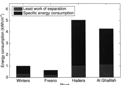
1-7 shows that SEC is usually 2-5 times greater than the least work of separation,

depending on system design aspects such as plant size and configuration. Areas with high water stress and low least work requirements are mapped to highlight regions with desalination potential. The least work of separation calculations are then used to develop simplified equations between least work and TDS, specific conductance, ionic strength and molality. Lastly, the thesis explores the impact of groundwater composition on the least work of separation, and the geographic distribution of TDS and well depth for 46,000 BGW samples and major ions for 28,000 BGW samples.

6 - Least work of separation Specific energy consumption

41--0 CP C: 02 CM C 0

A

Winters Fresno Hadera Al Ghalilah

Plant

Figure 1-7: Least work of separation as a percentage of specific energy consumption for two brackish water reverse osmosis plants (BWRO), Winters and Fresno, and two seawater reverse osmosis plants (SWRO), Hadera and Al Ghalilah. The darker regions represent the additional energy generated by irreversibilites in RO systems, primarily resulting from the driving pressure drop across the membranes. Data on

SEC, recovery ratio and feed and product salinities was obtained from DesalData [15]. Seawater composition was acquired from WHO [13]. Characteristic brackish

groundwater composition was acquired from USGS based on BWRO plant location

Chapter 2

U.S. Geological Survey major-ions

dataset

The U.S. Geological Survey (USGS) compiled a dataset of the major ions in ground-water in 2017 [14] to provide an updated summary of the occurrence of BGW and a more complete characterization of BGW resources. The dataset contains chemical, physical, and geographic properties of groundwater from 16 sources for approximately 124,000 groundwater samples across the continental U.S., Alaska, Hawaii, Puerto Rico, the U.S. Virgin Islands, Guam, and American Samoa. This paper uses brackish groundwater data from the continental U.S. only.

2.1

Coverage

The geochemical sources used to compile the major-ions dataset range from single publications to large datasets and from state studies to national assessments. Specific information on these sources can be found in Appendix A. Groundwater properties in the dataset include the concentrations of dissolved solids, major ions, trace ele-ments and radionuclides, pH, temperature, specific conductance, and density. Many of these properties are necessary to evaluate the least work of separation. Some sam-ples have missing density or bicarbonate and/or carbonate concentration data. In these cases, density was calculated using a well-established correlation for density,

temperature and salinity [16]. Alkalinity was converted to bicarbonate and carbon-ate concentrations according to methods outlined by Stumm and Morgan [171, using the Debye-Hiickel limiting law [18]. The dataset also contains a latitude and longi-tude pair for each sample, enabling geographic distribution analyses of groundwater characteristics.

Approximately 78,000 samples are freshwater (TDS < 500 mg/L) and 46,000 sam-ples are brackish water. Of the brackish samsam-ples, 28,000 have complete composition data, not diverging from electroneutrality by more than 5% 1. Groundwater samples are drawn from all 50 states. New Jersey, Delaware, Maryland, Texas, and North Dakota have the highest well/area densities (wells/km2_{) in the dataset, while}

Ken-tucky, Oregon, New Mexico, Alabama, and Vermont have the lowest in the dataset. North Dakota, South Dakota, Montana, Wyoming, and Nebraska have the highest well/population densities (wells/person) in the dataset, while Kentucky, Alabama, Georgia, Vermont, and Rhode Island have the lowest in the dataset.

2.2

Limitations

Although the dataset covers large areas across the country, it has some limitations.

USGS was unable to compile all available groundwater data for the nation,

particu-larly from local sources. The agency relied primarily on larger datasets available in a digital format from state organizations. In addition, well selection biases influence the type of groundwater data that is available. Well sites are not methodologically selected to characterize whole aquifers. Rather, they tend to be drilled in areas that have freshwater and/or a lower depth requirement to tap into the resource. This preference for freshwater and shallow wells results in a lack of comprehensive and consistent data. Consequently, the dataset does not represent a complete characteri-zation of BGW resources in the U.S.

The majority of samples have a TDS less than 500 mg/L, and there is an uneven

'The percent deviation from electroneutrality is calculated by summing over all of the cation

C and anion species A in the distributed solution, using the charge z of each species: pet err = 100 E4C (Z-C)1.(.-A)

distribution of wells across the 50 states, resulting in data gaps for many parts of the nation. The low correlation coefficient of 0.31 between state area and number of wells per state reflects that the occurrence of wells in a given area varies across states. This non-uniform well distribution may result partly from population density and total groundwater withdrawals in a given area. The correlation coefficients of number of wells per state, with state population and with total state groundwater withdrawals, are 0.53 and 0.60, respectively; these values indicate that number of wells in a state is related to these two parameters. Figure 2-1 shows the total groundwater withdrawals per state in 2010 versus the number of groundwater samples per state in the major-ions dataset. Texas and California have both the highest number of samples and total groundwater withdrawals, while Rhode Island and Vermont have the smallest number of samples and total groundwater withdrawals.

50 coCA

_L~

de

o

Figure 2-1: Total annual groundwater withdrawals per state in 2010 (data in

[2])

In order to fully characterize BGW resources, a larger amount of existing ground-water data must be compiled. New data that has a more extensive geographic reach

and less bias towards shallow and freshwater samples must be collected. Increased hydraulic analyses must be conducted.

Chapter 3

Methodology

The least work of separation is the benchmark energy consumption for any desali-nation system. It represents the minimum amount of work required to separate the supplied water into pure and brine streams leaving the desalination process, as determined for a thermodynamically ideal (reversible) process. The USGS data in combination with the mixed electrolyte Pitzer model [19, 20] is used to compute the difference in chemical potential [21] of these streams, which determines the least work of separation for each groundwater sample. In this thesis, the least work is calculated per unit of product produced (ri = 1 kg/s) and written as Wieast/mtp (kWh/M3).

3.1

Derivation of least work of separation

The least work of separation on a mass basis is derived from a control volume sur-rounding a black-box separator. The desalination system is modeled as a black-box separator with an inlet stream, the feed (f), and two outlet streams, the brine (b) and the product (p), as shown in Fig. 3-1. All streams have different salinities S.

A control volume is chosen far enough away from the separator that the inlet and

outlet streams are at ambient pressure and temperature, Te. The heat entering the system at environmental temperature is

Q,

Wsep

Q

Product

Feed Black Box

I

"nf, Sf Separator Brine

Tb, Sb > Sf

L---Figure 3-1: A control volume of a desalination system modeled as a black-box sepa-rator for deriving least work of separation.

Combining the first and second laws of thermodynamics on this control volume gives the rate of work for separation:

Wsep = Tlpgp + rnbgb - igf 9f + Te gen (3.1)

where g is the specific Gibbs free energy per kilogram of solution, rhi is the mass flow

rate of stream

j

Wleast = rnpgp + rnbgb - m5g9 (3.2)

Therefore, the difference between least work of separation and actual specific en-ergy consumption results from irreversibilities generated in real-world desalination systems. Entropy generation for thermal desalination systems primarily sources from heat transfer across a finite temperature difference, while entropy generation for mem-brane desalination systems mainly results from water transport through the high pressure drop across the membrane [22]. For a given salinity, water composition ef-fects do not substantially impact entropy generation [221. Conservation of mass for the mixture and the salts yields the least work of separation per mass flow rate of

product stream in terms of mass recovery ratio:

= (gp - gb) (gf - gb) (3.3)

MP r

where the mass recovery ratio is defined as the ratio of the mass flow rate of product stream to the mass flow rate of feed stream:

M =-(3.4)

rn f

We can gain more insight into the effect of physical properties on the least work of separation by rewriting Eq. (3.1) on a molar basis [21, 22J:

=east ( In aH_{2O,, +}

₍

2O In a

flH20,PRT alH2Qb asb

- ln aH2o + bs,f MH20 In as, (3-5)

i aHl2Q,b as,b

where M is molar mass, b is molality in mol/kg, subscript s represents all binary salt species in the mixture, a represents the activities of solutes and solvent in each stream, and the molar recovery ratio r is defined as the ratio of molar flow rate of water in product stream to molar flow rate of water in feed stream:

f = hH20,p

(3.6)

nH2o,f

Least work of separation is a function of feed and product composition, recovery ratio, and ambient pressure and temperature [21, 221. In this thesis, least work results are provided for a pure product (aH20,P = 1, b5,p = 1 in Eq. (3.5)) at atmospheric pressure

and evaluated at zero recovery. The USGS dataset includes the temperatures of each water sample, used in least work calculations. As recovery ratio approaches zero (i.e., infinitesimal extraction), least work of separation is minimized [21]:

n = lim Weast W1M t r-40

This is known as the minimum least work, and is the efficiency datum for drinking water desalination systems. This thermodynamic limit is equivalent to the removal of a drop of pure water from the ocean, which acts as a reservoir of chemical potential (analogous to a thermal reservoir in heat engine theory). Seawater from this reservoir is used as feedwater to the desalination system, and brine leaving the system is disposed into the same reservoir. Consequently, the feed and brine streams share the same chemical properties, resulting in identical Gibbs free energies [21]. The second term in Eqs. (3.3) and (3.5) becomes zero divided by zero. The mathematical proof in Appendix B shows that these terms limit to zero, so that Eqs. (3.3) and (3.5) reduce to the difference in Gibbs free energy of the product and brine streams:

Wmin_least

= (gp - 9b) _(3.7)

MP

For a sufficiently large BGW aquifer, brine disposal will not affect aquifer salinity, implying the aquifer acts as a reservoir of chemical potential in the same manner as the ocean. In such cases, the above physical argument holds for BGW desalination systems as well. However, the theoretical definition of minimum least work is gen-eral and does not require the actual presence of a disposal system for its validity. Thus, it remains a robust metric for describing the energy requirements to desalinate groundwater from any well.

3.2

Calculations

3.2.1

Evaluation of activity coefficients for least work of

sep-aration using Pitzer mixed electrolyte model

The Pitzer mixed electrolyte model [19, 23, 24 is used to calculate activities of solvent and solutes in each groundwater sample to determine the least work of separation.

The Gibbs free energy of a mixture is written as:

G = Znip (3.8)

where nr is the number of moles and pi is the chemical potential of species i. Chemical potential is:

pi = p' + RgTln(ai) (3.9)

where p4 is the chemical potential in the standard state, R9 is the universal gas

constant, T is the temperature, and ai is the activity of species i. The solute activity is defined on a molal scale as:

ai = yibi (3.10)

where bi is the molality of ion species i and N,i is the activity coefficient. The activity coefficient of an individual cation, M, is written as:

In -yM zMF + 1 ba(2BMa + ZOMa) a

+

S

c a

+

5 Z

a<a'

+ IZMI

5

C a n

For an individual anion, X, the equation is analogous to Eq. (3.11):

In Thx = zF + Eb,(2Bex + ZCex) C

+ E

+

> >

+

IzxI

E E

>3

The activity coefficient of an uncharged species N (e.g., aqueous C02) is given by:

In 7N = bc(2ANc) + ba (ANa) (3-13)

C a

The activity of water on a molal scale can be expressed as:

ln(aH2o) = MW(Z b-)q (3.14)

1000

Molal osmotic coefficient kb is computed from the expression:

(q-1) Emi = 2 [-AO I3/2

i 1 + 1. 2 -'f

+ >3bba(B + ZCa)

C a

+

c<c' a /

+ E babal (0a,1 + E bc1aa'c

a<a' \ c /

+ E

>3

>3 >3

n a n C

where z is the species charge, Z = EZ

Izilmi

X, and n represents uncharged (neutral) solutes. Summation over all i, c, a, and n

denotes a sum over all solutes, cations, anions, and neutral solutes, respectively. The summation notations c < c' and a < a' indicate that the sum should be carried out over all discernible cation pairs and anion pairs, respectively.

The following equations define the terms in the Pitzer equations for the activity and osmotic coefficients in aqueous solutions. The term F is based on an extended

Debye-Hiickel function [18]: __7 2

F=-AO

+

Z

beba

B'

+

b

,b,(

+ Z

(babaJb'ai,

(3.16)

It shows the characteristic first-order-square-root dependence on ionic strength result-ing from long-range electrostatic interactions. The parameter AO, which corresponds to the Debye-Hiickel limiting law, is written as:

AO = 1 e3

(27rNApH201

3 (1000,EkT) 1/2

where PH2o is the density of pure water, NA is Avogadro's number, kB is Boltzmann's

constant, and c is the relative permittivity of the solvent, which can be obtained from Uematsu and Franck [25]. The functions Bj, B8, B", and Cj represent the interactions between cations and anions:

BMx = 0( + /3 g(aMx v/) + /()g(12v/I) (3.18a)

B' =

0(l)g'(aMxVi)/I

0(2)g'(12v/Z)/I

B-X = 0( + 3(l exp (-amx Vi) + 0(2 exp (-12V'J) (3.18c)

CMX = 0 MX (3.18d)

2IzMzx 11/2

where aMX = 2.0 for 1-1 electrolytes and aMX = 1.4 for 2-2 and higher electrolytes. The parameters #(x are tabulated for a given ion pair. The parameter I#(X is related to complex formation and typically only has a non-zero value for 2-2 electrolytes. The

functions g(x) and g'(x) are given by:

g(x) = 2(1 - (1 + x)e-x)/x2 _(3.19a)

'()= 2

1

e

(3.19b)

9x W.2 2 ) _

The functions 'ij and @'V, represent interactions between like-charged pairs:

4i =

Oj

( EEI) (I)

(3.20b)

where Oij is the only adjustable variable for a given ion pair. The terms E9Oj (1)

and E_{6 (I) reflect excess free energy sourcing from electrostatic interactions between}

asymmetric electrolytes (i.e. ions with charge of same sign and different magnitude). They are dependent only on ionic strength and can be expressed as:

E ₉i(j) i ( J ij) - 1 - _(3.21a)

4122

E9 1 (I) ZZZJ (J1 (Xi,) - I

J

(3.21b)

1

1

X

Jo(x) - -- 1 - exp ( e- y2 _{dy (3.21c)}

4 xJ0 [ y

1 1 00X2

Ji(x) =

-

Xf1

-

+ e

exp

(--x

)

_dy

_(3.21d)

and xij is defined as:

xij = 6zizjA4v'Z (3.21e)

The integrals in Eqs. (3.21c) and (3.21d) can be evaluated numerically. In conclusion, the following parameters are adjustable: 3 to 4 per unlike-charged pair, 0(), 0(1,

CX; ne per