A decision-support model for managing the fuel inventory of a Panamanian generating company

A Decision-Support Model for Managing the Fuel Inventory

of a Panamanian Generating Company

by

Roberto Perez-Franco

Electromechanical Engineer, Panama Technological University, 2001

Submitted to the Engineering Systems Division in Partial Fulfillment of the Requirements for the Degree of

Master of Engineering in Logistics at the

Massachusetts Institute of Technology

May 7th 2004

(c) 2004 Roberto Perez-Franco, All rights reserved

The author hereby grants to M.I.T. permission to reproduce and distribute publicly paper and electronic copies of this thesis document in whole or in part.

Signature of Author

Engineering Systems Division May 9th, 2004

Certified by

Stephen Graves Abraham

J.

0 f I Thesis Supervisor Accepted by MASSACHUSETTS INSTMTTE OF TECHNOLOGY

JUL 2 7

2004

Director, Center tor I ransportation & Logistics Professor of Engineering Systems and of Civil and Environmental Engineering

A Decision-Support Model for Managing the Fuel Inventory

of a Panamanian Generating Company

by

Roberto Perez-Franco

Submitted to the Engineering Systems Division on May 7th 2004

in Partial Fulfillment of the Requirements for the Degree of

Master of Engineering in Logistics at the Massachusetts Institute of Technology

ABSTRACT

Bahia Las Minas Corp (BLM) is a fuel-powered generating company in the Panamanian power system. The purpose of this thesis is to design and evaluate a decision-support model for managing the fuel inventory of this company. First, we research BLM and its fuel replenishment methods. Then we define the problem, its objective function, assumptions, parameters and constraints. After identifying the most important given information (fuel price forecast, demand forecast, and current inventory levels), we define the equations that relate these inputs with the order sizes, and the availability and reserve constraints. Due to the large number of constraints, we devise a mechanism to calculate lower limits for the aggregate order sizes that prevent violations of the constraints beyond user-defined limits. We prepare a model in Excel for use with a single fuel type. This model takes stochastic forecasts of demand and fuel prices, and determines the best size for the weekly fuel order. After testing the model under several different scenarios, we conclude that it responds correctly to changes in price and demand. The complete discussion of these results can be found in the body of the thesis. Finally, we present some recommendations for BLM, both in relation to this replenishment problem and to its supply chain in general.

Thesis Supervisor: Stephen Graves

Title: Abraham

J.

to my loving wife, Monica, and my parents, Tito and Eka, optimal solution to the complex problem of my existence

Table of Contents

1.2.1. Brief history of BLM Corp, 9

1.2.2. Brief description of BLM's current generation capacity, 10 1.2.3. A word about BLM's future generation capacity, 11 1.3. Why optimize BLM's fuel inventory management? 12

1.4. Literature review, 13

1.4.1. On fuel inventory management for thermal generating plants, 13 1.4.2. On replenishment and inventory management in general, 14 1.4.3. On the economics and operation of power systems in general, 14

2. Understanding the Problem, 16 2.1. Problem Definition, 16 2.1.1. Objective, 16 2.1.2. Decision variables, 16 2.1.3. Constraints, 16 2.1.4. Assumptions, 17 2.1.5. Parameters, 19 2.2. Fuel demand, 22

2.2.1. Forecasting the required generation, 23

2.2.2. Translating generation into fuel consumption, 25 2.3. Fuel prices, 27

2.3.1. Fuel prices structure, 27 2.3.2. Fuel prices variability, 28

3. Building the model, 29

3.1. Equations, objective function and constraints, 29 3.1.1. Nomenclature, 29

3.1.2. Inputs, 32

3.1.3. General equations, 33

3.1.4. Weeks of relevance of the general equations, 34 3.1.5. Cost equations, 34

3.1.6. Objective function, 36 3.1.7. Original constraints, 36 3.1.8. Simplified constraints, 37

3.2. Implementing the model in Excel, 39 3.2.1. The spreadsheet, 40

3.2.2. The Macro, 46

3.2.3. Solver parameters and options, 49

4. Analysis of Results, 53

4.1. Using the model, 53

4.2. Example #1, 55 4.3. Example #2, 57 4.4. Example #3, 59 4.5. Example #4, 61 4.6. Example #5, 63 4.7. Example #6, 68 4.8. Example #7, 70 4.9. Example #8, 72 4.10. Example #9, 74 4.11. Unexpected results, 76

4.11.1. No added value in price forecast being stochastic, 76 4.11.2. Reserve violations are not constraining, 76

5. Conclusions and recommendations, 78 5.1. Conclusions, 78

5.2. Recommendations, 79

Appendix A -The Panamanian power system, 82

A. 1. Origin of the Panamanian power system, 82 A.2. Privatization of the Panamanian power system, 84 A.3. Current structure of the Panamanian power system, 85

A.3.1 Generation, 85 A.3.2 Distribution, 85 A.3.3 Retail Sales, 86 A.3.4 Transmission, 86 A.3.5 System operation, 86 A.3.6 Market operation, 87 A.3.7 Regulatory Institution, 87

Biographical Reference, 88

List of Figures

Figure 1 -Transformations to translate generation into fuel consumption, 25

Figure 2 - Screenshot of the whole spreadsheet, with labels over the four different areas, 40 Figure 3 - Screenshot of the Input-Output Area of the model, 41

Figure 4 - Screenshot of the Price-Related Area of the model, 43

Figure 5 - Screenshot of the extreme-left of the Demand-Related Area of the model, 43 Figure 6 - Screenshot of the center-left of the Demand-Related Area of the model, 44 Figure 7 - Screenshot of the center-right of the Demand-Related Area of the model, 45 Figure 8 - Screenshot of the extreme-right of the Demand-Related Area of the model, 45 Figure 9 - Screenshot of the Useful Metrics Area of the model, 46

Figure 10 - Excel Solver Parameters for the model - First six constraints are shown, 51 Figure 11 - Excel Solver Parameters for the model - Remaining constraints are shown, 51 Figure 12 - Excel Solver Options settings for the model, 52

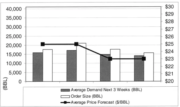
Figure 13 - Summary of the most important variables of Example #1, 55

Figure 14 - Graphical representation of demand, price and orders of Example #1, 55 Figure 15 - Summary of the most important variables of Example #2, 57

Figure 16 - Graphical representation of demand, price and orders of Example #2, 57 Figure 17 - Summary of the most important variables of Example #3, 59

Figure 18 - Graphical representation of demand, price and orders of Example #3, 59 Figure 19 - Summary of the most important variables of Example #4, 61

Figure 20 - Graphical representation of demand, price and orders of Example #4, 61 Figure 21 - Summary of the most important variables of Example #5, 63

Figure 22a - Graphical representation of demand, price and orders of Example #5, 63 Figure 22b - Total cost ($) versus the order size of Q2 (BBL), keeping Q1+Q2 constant, 65 Figure 23 - Summary of the most important variables of Example #6, 68

Figure 24 - Graphical representation of demand, price and orders of Example #6, 68 Figure 25 - Summary of the most important variables of Example #7, 70

Figure 26 - Graphical representation of demand, price and orders of Example #7, 70 Figure 27 - Summary of the most important variables of Example #8, 72

Figure 28 - Graphical representation of demand, price and orders of Example #8, 72 Figure 29 - Summary of the most important variables of Example #9, 74

Acknowledgements

Above all, I want to thank God for giving me this wonderful, undeserved opportunity to study among the best.

I want to thank my thesis advisor, Stephen Graves, who patiently guided me through the development of this project.

I also thank the staff of BLM Corp, who generously shared with me the information I required to prepare the model.

I am forever in debt with the Fulbright and Barsa scholarships, which supported my learning experience at MIT.

1. Introduction

1.1. Thesis overview

Bahia Las Minas Corp (BLM) is a generating company in the Panamanian power system. It runs a combined cycle powered by Marine Diesel and three steam turbines powered by Fuel Oil. In the future BLM expects to convert the steam turbines to coal. Every week, the managers of BLM decide on whether to place fuel orders from its supplier, and for how many barrels of each fuel type. These purchases represent tens of millions of dollars per year. Currently, there is no decision-support system to guide the decision-makers as to how many barrels of each type of fuel should be ordered at the time of placing the orders.

Our thesis is about designing a decision-support model for managing these weekly replenishment decisions. In order to avoid the need for new software, the model was designed to run in software with which BLM's staff is already familiar: Microsoft Excel 2002.

In Chapter 1, we introduce the reader to BLM Corp, review its history and its inventory management. We also explain briefly the purpose of a decision-support model for replenishment, and the importance it has for achieving a good inventory management, with high service level at the lowest cost.

In Chapter 2, we explore the replenishment problem, including the objective, variables, assumptions, parameters and constraints considered by the model. Among the variables presented in this section are two stochastic forecasts: fuel price and fuel demand.

In Chapter 3, we define the equations that describe the model, the objective function that is minimized, and the constraints that the model considers. Then we create the model,

by defining in an Excel spreadsheet the variables that are involved in the calculation and the

equations that relate these variables. The stochastic forecasts for fuel demand and fuel prices will also be included. We use the Excel Solver to find the order sizes that minimize the

relevant costs (storage cost, money cost and fuel cost), while respecting the constraints and considering the stochastic nature of the forecasts.

In Chapter 4, we analyze the performance of the model through nine examples. Finally, in Chapter 5 we summarize our findings and present some recommendations for BLM Corp, both in relation to this replenishment problem and to its supply chain in general.

1.2. Introduction to BLM Corp

In this section, we present an introduction to BLM Corp. A detailed introduction to the Panamanian power system, its origins, privatization and current structure, can be found in Appendix A.

1.2.1. Brief history of BLM Corp

When Panama's IRHE1 was privatized, one of the generating companies that were created was called EGEMINSA2_{. Later this name was changed to BLM Corp}3_{. The company} is named after Las Minas Bay and the port that is located in it, next to the generating units of the company. Fifty one percent of the stock of the company was purchased by Enron while 48.5% remained the property of the Panamanian government. Only 0.5% of the stock was purchased by employees. At the time of the privatization, nine generating units were

assigned to BLM:

1) Unit 1 (boiler and steam turbine.)

2) Unit 2 (boiler and steam turbine.)

3) Unit 3 (boiler and steam turbine.)

4) Unit 4 (boiler and steam turbine.)

5) Unit 5 (gas turbine.)

1 Institute of Hydraulic Resources and Electrification (Instituto de Recursos Hidriulicos y Electrificaci6n)

2 _{Empresa de Generaci6n Electrica Bahia Las Minas, S.A.} 3 Bahia Las Minas Corp

6) Unit 6 (gas turbine.) 7) Unit 7 (engines.)

8) Mount Hope (gas turbine.) 9) San Francisco (engines.)

Very soon, four of these units were dismantled, because of their obsolescence: Unit 1, Unit 7, Mount Hope and San Francisco. At the same time, BLM Corp inherited from IRHE the plans of a new generating complex. This plan included a new gas turbine (Unit 8) and a new steam turbine (Unit 9): the three gas turbines (Units 5, 6 and 8) would supply their exhaust gas to the new steam turbine (Unit 9) in order to operate the complex as a Combined Cycle. BLM Corp implemented this plan, and the Combined Cycle was operating

by 1999. In December 2000, lightning struck Unit 6 and put it out of service for six months.

1.2.2. Brief description of BLM's current generation capacity

Currently, BLM Corp encompasses seven generating units, which we can classify in two groups: the steam turbines and the combined cycle.

Steam turbines

There are three steam turbines (units 2, 3 and 4). Each has an original plate capacity of 40 MW. Currently, their gross capacity is around 35 MW. These units run on Fuel Oil No 6 (Bunker C). Running at full capacity, each steam unit requires around 1,300 barrels of No 6 per day. They burn Light Diesel during start-up.

Combined cycle

The combined cycle includes one steam turbine (unit 9) and three gas turbines (units 5,

6 and 8). Unit 5 has a plate capacity of 33 MW. Unit 6 has a plate capacity of 33 MW. Unit 8

has a plate capacity of 34 MW. Unit 9 has a plate capacity of 58 MW. The combined cycle has a plate capacity of 158 MW, although currently its gross capacity is around 147 MW. The gas turbines run on Marine Diesel No 2. For its use in BLM's turbines, Marine Diesel

includes 80% of Light Diesel and 20% of Fuel Oil No 6. The gas turbines burn Light Diesel during start-up. The complex can operate in six different configurations:

1) Unit 5 can operate as an independent gas turbine, with a gross capacity of 32 MW.

2) Unit 6 can operate as an independent gas turbine, with a gross capacity of 32 MW.

3) Unit 8 can operate as an independent gas turbine, with a gross capacity of 33 MW.

4) One gas turbine can operate with Unit 9 as a combined cycle, with a gross capacity of approximately 49 MW.

5) Two gas turbines can operate with Unit 9 as a combined cycle, with a gross capacity

of approximately 98 MW.

6) Three gas turbines can operate with Unit 9 as a combined cycle, with a gross capacity

of approximately 147 MW. Running at full capacity, the combined cycle requires around 4,500 barrels of No 2 per day.

Thus, the total plate capacity of BLM is 278 MW, which is 20% of the total 1.38 GW of installed capacity available for the Panamanian system, and 33% of the current maximum demand of the country (0.85 GW).

1.2.3. A word about BLM's future generation capacity

Since the beginning, BLM Corp has considered the use of less expensive fuels. One of the ideas the company considered at the beginning was to run the combined cycle on natural gas. However, since Panama has no wells of natural gas, it would have to be brought from abroad. Liquefied Natural Gas was too expensive. Enron had planned to invest $300 million in an underwater natural gas pipeline from Cartagena, Colombia to the Bahia Las Minas plant, 3 feet in diameter, almost 600 kilometers long. The pipeline would initially transport 70 million cubic feet (MCF) per day. However, an increase in the projected cost of gas rendered the project unprofitable for the investors, and it was scrapped.

The current plan is to build a new, 120 MW fluidized-bed boiler to burn pulverized coal. This boiler will supply steam to Units 2, 3 and 4. At a cost of 100 million dollars, this boiler should be ready by July 2006. The company estimates that using coal instead of Fuel Oil will cut the variable cost of these units by half, which will increase BLM's ability to compete in the Panamanian generation market.

The coal BLM plans to use, which would be brought from Colombia, has a sulfur content of 0.7%. This represents a gain from an environmental perspective, because the Fuel Oil currently in use has 3.0% content of sulfur. The new boiler will also be furnished with pollution-abatement technology. The terminal to receive coal in the Las Minas bay port was inaugurated in early February 2004. BLM has considered keeping the capacity to burn either coal or fuel oil in this boiler, which would allow the company to choose the fuel that is less expensive at any given time.

1.3. Why optimize BLM's fuel inventory management?

Generally speaking, the goal of inventory management optimization is to reduce the relevant costs, including purchase cost and holding cost, while providing the desired product availability.

For an electricity generating company, the goal of fuel inventory management is to balance the cost of purchasing fuel and holding it in inventory against the risk of not having enough fuel available to satisfy demand in real time. In the case of BLM, most uncertainty is associated with fuel demand, although fuel supply is not necessarily certain. BLM must keep fuel inventory at proper levels to avoid running out of fuel, without building excessive inventory levels.

Also, since fuel prices are not fixed, it is possible to take advantage of price changes. When fuel price is expected to increase substantially, it is desirable to build a stock of fuel

purchased at the present low prices, to avoid the purchase of more expensive fuel in the near future.

Thus, the purpose of optimizing BLM's fuel inventory management is to prevent unnecessary fuel purchases and inventory accumulation, to take advantage of variations in fuel prices, and to ensure the availability of fuel, both stored and ordered, to satisfy availability and reserve expectations, at the lowest possible total cost.

1.4. Literature review

1.4.1. On fuel inventory management for thermal generating plants

Some of the publications that discuss topics similar to that of our work include the following:

"A Utility Fuel Inventory Model", published by Peter A. Morris et al. in Operations

Research, Vol. 35, No. 2 (Mar.-Apr., 1987), 169-184. This paper discusses an inventory modeling system, called "The Utility Fuel Inventory Model, or UFIM, which was designed to help electric utilities set a long-term fuel inventory strategy that specifies the most cost-effective inventory levels to maintain during normal times (e.g. times when there are no disruptions). Morris's paper describes the model, its use and one of its first applications. He mentions that UFIM was used at that time by more than 50 utilities.

"A System Integration and Optimization Model for Fuel Management and Scheduling of

Power Generators", doctoral thesis of Babul Patel, presented in 1981 at the University of Nebraska. Patel examines the problem of scheduling power generators and develops a dynamic programming technique to obtain an optimal dispatch schedule. The final results of his analysis include weekly or monthly summaries of the unit's fuel inventory and fuel costs.

"Studies in fuel supply and air quality planning by electric utilities", doctoral thesis of Yung-Tang Shen, presented in 1996 at Ohio State University. Shen develops a

comprehensive linear programming model for air quality and fuel management, dealing with fuel purchases, consumption, inventory, and air quality control strategies. He considers, among other variables, inventory requirements and electricity demand. His objective was to minimize total fuel purchase, inventory, and air quality control costs over a given planning horizon.

1.4.2. On replenishment and inventory management in general

The literature on replenishment and inventory management is vast and specialized. Our model uses rather basic concepts. For the reader that is not familiar with the general concepts of inventory management and wants to acquire more knowledge on this area, we list the names of two books that will prove helpful.

The first is "Inventory Management and Production Planning and Scheduling" by Edward A. Silver, David F. Pyke and Rein Peterson. This book was repeatedly recommended to us during the MLOG program. It tries to close the gap between the theoretical advancements and the industrial applications of inventory management.

Another excellent book, which deals with Supply Chain Management as a whole, is "Supply Chain Management", by Sunil Chopra and Peter Meindl. The replenishment techniques described in this book for unique products with stochastic demand (Chapter 9) were very helpful for developing our model, since it considers stochastic variables.

1.4.3. On the economics and operation of power systems in general

Although power systems are not the core subject of our thesis, we realize that some of the readers of this document will be interested in learning more about them. There is a vast literature regarding the operation, economics and risk management of power systems. We want to recommend four of them.

As an introduction to the engineering and economic factors involved in operating and controlling power generation systems, our recommendation is "Power Generation,

Operation and Control" by Allen

J. Wood and Bruce F. Wollenberg. This book covers

For the reader interested in power market, we recommend two excellent books. The first is "Power System Economics", by Steven Stoft, which introduces key economic, engineering and market design concepts for power systems, and explores in more depth specific areas of interest in power markets. The second book is "Market Operations in Electric Power Systems", by Mohammad Shahidehpour, Hatim Yamin and Zuyi Li, which discusses market structure, operation, forecasting, scheduling, and risk management in electric power systems. It dedicates one whole chapter to one of the topics we mention in Appendix A: short-term load forecasting.

Readers interested in exploring the risk management techniques available to power companies are invited to read "Energy and Power Risk Management", by Alexander Eydeland and Krzysztof Wolyniec. Although not related to the core subject of this thesis, risk management techniques such as modeling, pricing and hedging, can complement our inventory management approach to protect generating companies from fuel prices volatility.

2. Understanding the Problem

2.1. Problem Definition

2.1.1. Objective

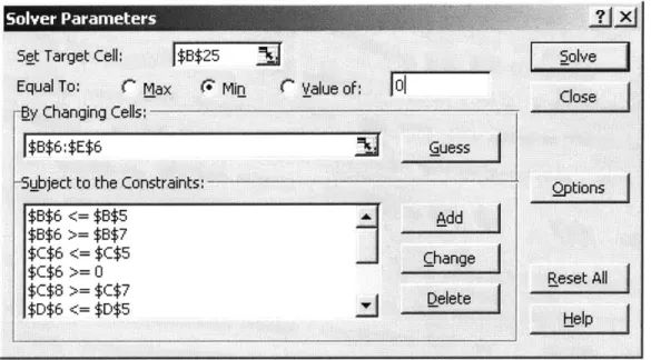
We can define the problem as follows: create in Excel an inventory optimization model for BLM that determines, for a single fuel type, the size of next week's fuel order, so that the purchase and holding costs are minimized considering a horizon of four weekly orders into the future, while respecting all constraints and assumptions.

As we stated before, the way we will create this model is by defining in an Excel spreadsheet the relevant variables (including the stochastic forecasts for fuel demand and fuel prices) and the equations that describe the model. We will not write our own optimization code. Instead, we will use Excel Solver to find the order sizes that minimize the relevant costs (storage cost, money cost and fuel cost), while respecting all constraints.

2.1.2. Decision variables

The decision variables are the only variables that can be adjusted by the model to minimize the objective function. These variables are the size of the weekly orders for the next four weeks, which are the relevant orders within the horizon of the model. The sizes of the orders are subject to the constraints of the model.

2.1.3. Constraints

While minimizing the objective function, the model should consider the following constraints:

1. For each week in the horizon of the model, order sizes cannot be negative.

2. For each week in the horizon of the model, order sizes cannot be larger than a maximum size specified by the user. The purpose of this upper cap is to account for the limitations in:

a. The financial capacity of BLM to purchase fuel.

b. The fuel availability of the supplier.

3. For each week in the horizon of the model, the probability of a stockout should

be no more than the maximum acceptable probability specified by the user. This assumption is based on the significant penalties of stockout.

4. For each week in the horizon of the model, the probability of fuel reserve levels falling below the expected reserve level should be no more than the maximum acceptable probability specified by the user. Fuel reserve is not a hard constraint (as proven by the fact that, in times of shortage, the reserve has been lower than the expected reserve levels), but it is considered a best-practice criterion that should be respected whenever possible.

a. Fuel reserve is defined as the sum of the fuel stored both in the local and external storages plus the fuel of orders that have already been placed (even if this fuel is not physically "in transit").

b. Expected reserve is defined as the fuel needed for the next 10 days of

forecasted generation.

If the model is asked to decide the order sizes so that there is no probability of availability or reserve violations, the model will make its replenishment decision based on the scenario with the greatest demand. This results in the model recommending very high order sizes, which is not desirable. Accepting a probability of violations greater than zero tempers these results. That is why the model will ask the user to provide values for the maximum accepted probabilities for violations of availability and reserve for each week.

Please notice that there are no constraints related to fuel prices.

2.1.4. Assumptions

1. The cost of placing an order is negligible. The rationale for this assumption is

that the only variable cost of placing an order is the cost of the bank transfer, which is negligible compared to the amount paid for the fuel itself. Other costs, such as those related to staff and fuel transportation, do not depend on the number of orders placed.

2. We assume that one order for each fuel type is placed every week, and that the size of each order is decided on Friday afternoon4. Of course, BLM can decide to place an order for 0 barrels (e.g. to place no order) on any week.

3. We assume that the first barrel of an order arrives one week later, and the last

barrel two weeks later, counting in both cases from the Friday the size of the order was decided.

4. Once an order is placed, it cannot be modified. This assumption is based on information we received from BLM describing its relationship with the supplier.

5. The shipping capacity of the supplier is not considered a constraint. The

receiving capacity of BLM is discussed in section 2.2.

6. The storage capacity of the supplier is not considered a constraint. The storage

capacity of BLM is discussed in section 2.2.

7. All orders of both Marine Diesel and Fuel Oil are delivered by truck.

8. There is no correlation between short-term variations in fuel price (e.g.

variations in price in the following four weeks) and variations in fuel consumption. This assumption is based on the experience of BLM staff, and is supported by the fact that in Panama, most thermal generating units receive their fuel from the same markets: the variations in fuel prices are felt almost equally by all generating companies. Also, the percent of hydroelectric

4 In real life, BLM places the orders any day of the week, but to keep the model simple, we assume that orders are placed only on Friday afternoon.

generation at any given time depends on long-term forecasts of fuel prices, but is not affected by variations of fuel prices in the short run. Therefore, short-term variations in fuel prices have no noticeable effect over unit commitment and

required generation.

9. At any given time, BLM knows the current fuel inventory levels. BLM has no

real-time reading of the fuel levels in its tanks. However, these levels are measured directly in the tanks once a month, and between the readings the levels in the tanks are estimated based on the actual generation and heat rate of the units, and the heating values of the fuel.

10. BLM decides on Friday the size of the order for each fuel type for next week

only. However, the planning horizon for the model includes the demand forecast for the next six weeks and the order sizes for the next four weeks. This planning horizon is a compromise between anticipated planning and forecast reliability:

a. On the one hand, using more than four weekly orders as decision variables would require using more than six weeks of demand forecast. This is not desirable, because forecasts for demand so far in the future are not reliable.

b. On the other hand, using less than four weekly orders as decision

variables would severely impair the model's ability to play with inventory levels for the company's benefit, i.e. to purchase excess fuel inventory at lower prices in the present to avoid purchasing fuel later at higher prices.

2.1.5. Parameters

Our model will consider the following parameters, which are presented here with the values of the current supplier. In the future, if these values change, they can be updated in the model.

1. Number of suppliers: Currently BLM has only one fuel supplier.

2. Demand: A stochastic fuel demand forecast is used as input to our model. By

stochastic demand forecast, we mean a forecast that has, for each one of the

following six weeks, fifty possible demand scenarios, each with a probability of 2%. This demand forecast is calculated by BLM based on a stochastic optimization run by the system operator (National Dispatch Center' or CND), in a computer program called SDDP. In section 2.2, we discuss how this demand forecast is prepared.

3. Fuel prices: A stochastic fuel price forecast is used as input to our model. By stochastic price forecast, we mean a forecast that has, for each of the following

four weeks, five possible price scenarios, each with a probability of 20%. This price forecast is calculated by BLM's staff. Later in this chapter, in section 2.3, we discuss the structure and variability of fuel prices. Fuel price information of BLM is confidential. As we mention in Chapter 4, the same results are achieved by using either a deterministic or a stochastic price forecast.

4. Local storage capacity: BLM has a local storage capacity of 50 thousand barrels of Fuel Oil and 50 thousand barrels of Marine Diesel. As a reference, consider that when the generating units of BLM are operating at full capacity, they require each day around 4 thousand barrels of Fuel Oil for all the three steam units and 4.5 thousand barrels of Marine Diesel for the Combined Cycle. However, very seldom are all units generating flat out. Local storage capacity is a sunk cost. This cost is not relevant for our calculations.

5. External storage capacity: Theoretically, it is possible for BLM to lease additional

storage capacity from its supplier, for a fee. Since BLM has never used this service before, there is no information about the exact cost of this service. For

the sake of our model, we have assumed a cost of $2/BBL-week, that is, two dollars per barrel stored per week stored, paid on the maximum amount of barrels stored each week (not on the average amount of barrels stored.) As we will explain later, for our model weeks start on Saturday.

6. Cost of money: The holding cost is composed of the cost of external storage

capacity and the cost of money. BLM informed us that its cost of money can be expressed as LIBOR6 plus a confidential constant. For our model, we estimated that the money cost is 25% per year, or 25%/(52 weeks/year) = 0.481% per week.

7. Order lead time: Order lead time depends on the size of the order. According to

BLM, for an order of 25 thousand barrels of one type of fuel, from 10 to 12 days elapse from the moment the size of the order is defined to the moment the tank trucks are received at the plant. This delay can be divided into three periods:

a. Three days elapse from the moment the size of the order is defined to the moment the bank emits the purchase order. This delay does not depend

on the size of the order.

b. Between 3 to 4 days elapse from the moment the purchase order is

emitted and the moment the supplier sends the first loaded tank truck. Part of this time is used to get a tax exemption for the fuel.

c. The rest of the delay depends on the size of the order. In the past, the average order of BLM has been of 25,000 BBL of each fuel. For an order of this size, 4-5 days elapse from the moment the first truck leaves the supplier's premises and the moment the last truck arrives at BLM's plant.

To account for the fact that orders can be larger than 25,000 barrels, and to compensate for any unforeseen authorization, processing or delivery delay, we will consider the

whole lead time to be two weeks (14 days) from the day the order is decided to the day the last tank truck arrives at BLM's plant.

8. Based on the structure of the delays, we make the following assumptions:

a. For the sake of calculating the cost of money, we assume that BLM takes financial responsibility of the fuel (e.g. must have separate funds for them) from a day after the amount of the order has been decided. Since the sizes of the orders are decided on Friday, BLM would pay the cost of money starting the following day, Saturday, which is the first day of the new week.

b. For the sake of calculating the cost of storage, we assume that BLM must

assume physical responsibility for the fuel starting one week after the day the supplier has cleared this fuel for delivery. Speaking in terms of days after the Friday the order size is determined: the fuel is BLM's responsibility 2 weeks after the order has been placed.

9. Receiving capacity: BLM can receive up to 30 tank trucks per day for each type

of fuel, each truck with an average of 202 BBL of fuel. This amounts to a maximum receiving capacity of 6,060 thousand barrels per day for each type of fuel. Since BLM's fuel consumption at full capacity is smaller than its receiving capacity, the receiving capacity is not a constraint for our decisions.

10. We assume that demand is uniform during the week. It is a known fact that

generation on Saturdays and Sundays is usually lower than on weekdays, but in order to keep our model reasonably simple we will neglect this difference.

2.2. Fuel demand

Forecasting the fuel consumption of BLM is a complex process, since it depends on a variable that is very hard to forecast: the required generation of BLM.

For our model, we do not attempt to prepare our own fuel consumption forecasts. Instead, we use the forecasts prepared every week by the system operator. Section 2.2.1 explains how the system operator forecasts the required generation of BLM's units. Section 2.2.2 explains how these generation forecasts are translated into fuel consumption forecasts.

2.2.1. Forecasting the required generation

As we mentioned in section 1.2.3., the required generation of BLM depends, generally speaking, on two factors: unit commitment and system-wide energy demand. System-wide energy demand occurs in real-time, and has been found to depend on several factors, including: 1) the amount of installed load in the system (nation-wide), 2) the time of the day, 3) the day of the week, 4) whether a day is a holiday, 5) the week of the year, and 6) weather (fresh, rainy days have lower demand than hot, sunny days). Unit commitment is determined by the system operator (CND), who decides to commit a unit depending on many factors, including but not limited to the following: 1) the availability of the generating unit, 2) the variable cost of all the available generating units in the system, 3) long-term weather forecast (in a rainy year hydroelectric units are used more than in dry years), 4) the long-term fuel prices forecast, 5) the expected demand for the day, the week, the month, and the next two years, 6) the start-up cost and operation restrictions of the generating unit, and 7) the stability and safety of the operation of the system.

Obviously, trying to forecast the required generation based on expected energy demand and optimal unit commitment is a very complex task and is beyond the scope of our model. Instead, we will use the forecasts prepared every week by the system operator, CND, with the help of all the stakeholders of the system. These forecasts are used to determine many things, including the operative planning of the system for the short and long terms. They are

highly regarded as accurate forecasts for the short-term operation, because they are prepared

with the active collaboration of all parties involved, including representatives of the staff of BLM Corp and all the other generating companies.

Every Thursday, before 10:00 AM, the generating, transmission and local distribution companies give CND large amounts of information regarding the status of their equipment, including scheduled maintenances and other relevant data. For example, LDCs give CND the energy demand forecasts for their networks; thermal generators give CND their generation variable cost for the week, based on the current fuel prices; weather experts forecast inflows to the reservoirs for the next two years; ETESA gives CND the information on scheduled transmission interruptions because of network maintenance.

With this information, and the use of specialized software called Stochastic Dual Dynamic Programming (SDDP), CND performs three analyses. Each one of these analyses provides as output a large amount of information, including a forecast of the generation that will be required from the units of BLM Corp. The three analyses are:

1) The Stochastic Run. This run uses 3 years of data. It considers reservoir inflows (the

amount of water that enters the reservoirs) stochastically, and prepares fifty hydrologic scenarios based on historic data from several decades. SDDP uses dynamic programming to determine the optimal prices ($/MWh) that should be assigned to the hydroelectric generating units in order to balance their generation, on an economic dispatch basis, with the generation of thermal units. This run provides us with a stochastic forecast of BLM's required generation for every week of the next three years, in GWh. The forecast is stochastic because it considers 50 possible weather scenarios, which translates into 50 possible generation scenarios for BLM, each with a probability of 2%. History teaches that

the forecasts of the first four weeks are very accurate.

2) The Week-Ahead7 _{Deterministic Run. CND prepares its operative policy using the}

optimized hydroelectric generation prices obtained from the first run. Considering both these prices and the thermal prices, CND performs a short-term analysis, hour by hour, to determine unit commitment for the next week (from Saturday to Friday). This unit

commitment will be used as reference in real-time for the economic dispatch of the system, constrained by safety and stability considerations. This run provides a deterministic forecast of the BLM's required generation for every hour of the next week, in MWh.

3) The Month-Ahead8 Deterministic Run. CND performs a third analysis, using a horizon of two years, with weekly steps, considering weather as a deterministic variable. In the words of Percy Garrido, BLM's senior analyst in charge of SDDP operation, the purpose of this run is to "provide a robust forecast of the next four weeks". The forecast is not considered accurate beyond the fourth week. This run provides us with a deterministic forecast of BLM's required generation for every week of the next month, in GWh.

Every Friday morning, representatives from all the stakeholders of the power system, including BLM, gather in an office at CND's headquarters and discuss the results of these three runs. As a result of this weekly meeting, any discrepancies and errors that are detected in the runs prepared on Thursday will be corrected by CND on Friday noon. Thus, every Friday afternoon all the companies (including BLM) have access to the final forecasts from the three runs of SDDP performed by CND and verified by the all parties.

2.2.2. Translating generation into fuel consumption

For the sake of inventory management, demand should be expressed in terms of fuel units (e.g. BBL), instead of electrical energy (e.g. MWh). It is possible to translate the forecast of required generation into one of fuel consumption. As a matter of fact, the SDDP software makes this automatically. Let us review the logic behind this transformation. The following figure illustrates the calculation process.

Generation Heat Rate , Energy Heating Value ,Fuel Consuption

(MWh) (MWh/MBTU) (MBTU) (MBTU/BBL) (BBL)

Figure 1 -Transformations to translate generation into fuel consumption.

Generation is given in Watts-hour or its multiples, such as MWh or GWh. For the purpose of fuel replenishment, it is useful to express fuel consumption in the units used in the purchase orders. In the case of liquid fuels, such as Fuel Oil and Marine Diesel, these units are either gallons or barrels (BBL). In the future, when coal is used in BLM, the consumption of this fuel will likely be expressed in tons.

Energy is the link between generation and fuel consumption. In the Panamanian power system, energy is commonly expressed in terms of MBTU (millions of BTU).

The variable that allows us to determine how much energy is needed to obtain a certain generation from a specific generating unit is known as Heat Rate, but is also called "Efficiency", and is expressed in terms of MBTU/MWh. Each generating unit of BLM, even each configuration of the Combined Cycle, has an efficiency curve, which expresses the efficiency of the unit at any given generation level.

The variable that allows us to determine how much energy is contained in a unit, i.e. barrel or ton, of a given fuel is the Heating Value, which can be either gross or net. In Panama, it is commonly expressed in MBTU/BBL.

Every week, CND inputs into SDDP the values of Heat Rate for every generating unit of the system, including the three steam units and all the configurations of the combined cycle of BLM. These values are updated every year or so, after efficiency tests made by third-party engineering firms. CND also inputs into SDDP the Heating Values for the specific fuel that every generating unit is using in a given week. This allows SDDP to translate, through simple calculations, the forecast of required generation into a forecast of fuel consumption. After the Stochastic Run, the SDDP software returns its fuel consumption forecast in a file called fuelcn.csv. This file contains, among other values, the two stochastic forecasts of fuel consumption for BLM: one for Fuel Oil and one for Marine Diesel. For each fuel, for each one of the following 52 weeks, SDDP forecasts 50 possible consumption scenarios (divided

in four blocks), each with a probability of 2%. These forecasts are expressed in thousand of gallons of consumption per week (not in barrels).

However, it is necessary to make an adjustment to this forecast before we use it in our model. SDDP calculates the forecast considering that the generating units operate all the time at the maximum efficiency point of their efficiency curves. However, in real life they sometimes operate at lower efficiency points that consume more fuel for the same generation output. BLM's Garrido has told us that by augmenting the forecasted values of consumption by 5% we can compensate for this deviation.

Our model uses this stochastic forecast, with the 5% efficiency adjustment and transformed to barrels, as input for its calculations. Note: blocks are not used individually.

2.3. Fuel prices

2.3.1. Fuel prices structure

Confidentiality prevents BLM from sharing with us the fuel prices of the contract with its current supplier.

However, they shared with us the structure of the formula that determines these prices: they are calculated as the monthly average of the prices of the fuel in the US Gulf according to Platt's Latin Wire, plus a fixed amount that was not disclosed. Unfortunately, the information contained in Platt's Latin Wires is available only to subscribers of this service and cannot be shared with non-subscribers.

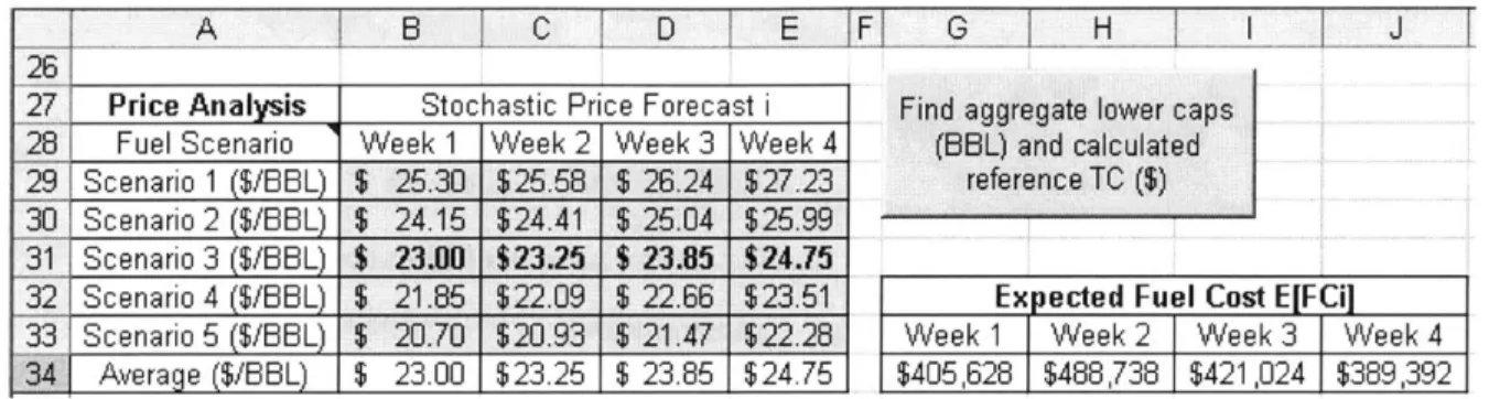
When the model is in use in the future, BLM will provide as an input a stochastic price forecast for each fuel type. By stochastic price forecast we mean a forecast that has, for each of the following four weeks, five possible price scenarios, each with a probability of 20%.

For the purposes of our thesis, we will use arbitrary fuel values between $23/BBL and $27/BBL, which, based on my experience in BLM, are typical values.

2.3.2. Fuel prices variability

To develop our model, we do not need to know the exact values of fuel prices. However, to be able to prepare examples to evaluate our model, it helps if we know the magnitude of variation that these fuel prices usually display. Based on our experience in BLM, and using as a reference publicly available WTI oil prices for the last 12 months, we have estimated that in the absence of high-profile world scale events, it is common for BLM to suffer changes of fuel price of 8% from one month to the next. To estimate how extraordinary events, such as the recent wars in Iraq and Afghanistan, can increase the price variations, we used data from February and March 2003 (near the beginning of the latest war in Iraq). Prices in these months show that the variability could reach values of up to 18% under these circumstances.

3. Building the model

In section 3.1 we define the equations that describe our model. In section 3.2 we simplify the constraints of the model by defining aggregate lower limits for the order sizes. In section 3.3 we describe the development of the Microsoft Excel model.

While you read this chapter, please keep in mind that the model we develop works with a single type of fuel, which can be either Fuel Oil or Marine Diesel. Therefore, BLM would have to run two copies of the model, one for each fuel. If the "barrels" labels are replaced with "tons" labels, the model can be used for coal, too.

3.1. Equations, objective function and constraints

3.1.1. Nomenclature

In this section we define the nomenclature that we will use later to write the equations that describe the problem, in three groups: 1) general nomenclature, 2) nomenclature of input variables, and 3) nomenclature of calculated variables. The text inside the parenthesis indicates the units this variable will have in our model.

As you read this section, keep in mind that the demand forecast has 50 stochastic scenarios and the price forecast has 5 stochastic scenarios.

3.1.1.1. Nomenclature - General nomenclature

" Weeks in the Panamanian power system start on Saturday and end on Friday. This type

of week is called "planning week" or " Titistic week", and is used in our model because it is used in the input data we receive from SDDP.

" n is an integer representing the number of weeks considered in the horizon of the

model. In our model, n is four (4) weeks.

* j is an integer that represents every given demand scenario, from 1 to 50, of the

stochastic demand forecast, each with a 2% probability.

* k is an integer that represents every given price scenario, from 1 to 5, of the stochastic price forecast, each with a 20% probability.

* Q is the amount of fuel purchased in the order of week i (BBL). The decision of the exact size of this amount is made on Friday of week i-1. According to our assumptions, this amount is part of BLM's fuel reserve since the first day of week i, but is physically in BLM's storage starting in the first day of week i+2. The sizes of the past two orders, Qi and Qo, are input variables that should be provided by BLM. On the other hand, the order sizes from weeks from Qi to Qn are decision variables, and are identified collectively in this thesis as Q.

3.1.1.2. Nomenclature - Input variables

* LC is the local fuel storage capacity of BLM (BBL). Storing fuel locally implies no relevant cost for our calculation, since there is no variable cost associated with it.

" Do is the fuel demand in week zero. This is a single value from the past provided by BLM

as input.

" Dij is the fuel demand in week i in demand scenario

j. These values originate in the 50

scenarios of CND's Stochastic Run of SDDP, and are later transformed to barrels and increased by 5% to be used as input values to the model. As we explained at the end of section 2.2.2, the 5% adjustment compensates for the fact that efficiency under real generation conditions is lower than the optimal efficiency used by SDDP for its forecast.

* CFii is the cost of the fuel in week i in price scenario k ($/BBL)

" CFi is the average cost of the fuel in week i for the five price scenarios ($/BBL)

" CE is the cost of leasing the external storage space for a week ($/BBL-week). We assume

the cost is charged to the maximum amount of fuel stored each week i.

* MQ is the maximum or upper cap to the value of Qi (BBL).

" MVAi is the maximum acceptable probability of violation of the availability constraint

(e.g. stockout) in week i, specified by the user (%). For our model, we assumed 20% for all weeks.

" MVRi is the maximum acceptable probability of violation of the expected reserve

constraint in week i, specified by the user (%). For our model, we assumed 20% for all weeks.

3.1.1.3. Nomenclature - Calculated variables

" TSij is the maximum amount of fuel that is stored both locally and externally in week i in

demand scenario

j

" LSij is BLM's maximum requirement for local fuel storage in week i in demand scenario j (BBL). This value occurs at the beginning of week i. The purpose of this variable is to simplify the calculation of ESij.

" ESij is BLM's maximum requirement for external fuel storage in week i in demand

scenario j (BBL). This value occurs at the beginning of week i.

" Aij is the minimum amount of fuel that is physically available for generation in week i in

demand scenario j (BBL). This value occurs at the end of week i. The minimum of fuel that is locally available is calculated accounting for the fact that as soon as 7 days after the order is placed, fuel is arriving at the plant in tank trucks.

" VAij is a variable created to know if the value of Aij is violating the "no stockout"

than zero. A violation is indicated by a value of VAij = 1, while no violation is represented by 0.

" Rij is the minimum reserve of fuel inventory in week i in demand scenario j (BBL). This value occurs at the end of week i. Fuel reserve is understood as the sum of the fuel stored both in the local and external storages plus the fuel of orders that have already been placed.

" ERij is the minimum expected fuel reserve that the regulations expect BLM to have,

equal to the forecasted demand of the next ten days (BBL).

* VRj is a variable created to know if the value Rij is violating the minimum expected reserve constraint ERj, e. g. that at any given time the fuel reserve Rij should be more than the minimum expected reserve ERj. A violation is indicated by a value of VRij = 1, while no violation is represented by 0.

" FC is the expected cost of fuel over the entire horizon of the model ($).

" SC is the expected cost of external storage over the entire horizon of the model ($).

" MC is the expected cost of money over the entire horizon of the model ($).

" TC is the sum of the expected relevant costs: simply the sum of FC, SC and MC ($).

3.1.2. Inputs

Let us define week 1 as the week for which we need to determine the order size. Our model is designed to be run on the last day of week 0 (Friday), to decide the size of order Qi. In this section we list the information that our model uses as input, which should be provided by BLM before running the model.

" LC: The local storage capacity, (BBL).

e _{CM: The cost of money per week, (%-week).}

"

Q1,

* TSo: The maximum amount of fuel that BLM had stored both locally and externally in week zero (BBL). In other words, it is how many barrels of fuel BLM had stored both locally and externally last Saturday (the first day of week 0).

" CFik for i={1,4} and k={1,51: the five stochastic forecasts of prices for the following four

weeks, starting in week 1 ($/BBL).

" Do: The demand of week zero (BBL). On Friday afternoon, this demand is known for the

last 6 days, and only the demand of the last day has to be estimated. Do is a single value.

* Dij for i={1,6} and j={1,50}: the demand forecast for the 50 stochastic scenarios of the next six (e.g. n+2) weeks, starting in week 1 (BBL).

" MQi for i=[1,4}: the upper cap to the value of Qi for i=[1,4} (BBL).

* MVAi for i={1,41: the maximum acceptable probability of availability violation (%).

" MVRi for i={1,41: the maximum acceptable probability of reserve violation (%).

3.1.3. General equations

The following equations define the variables of the model that are not given as input.

TSi

TS

+

Q-2

-,

LSU = Min(TS

, LC)

ES.. =TS.. - LS.

A.

=LS.. - D.

e1

As<

0

0,) otherwise

Ri, =

(TS

+

Q-

_+

Q,)-

Di

3

ERU

=Di

+-3Di+,

F1,

Ri. <ER.

V

j

0, otherwise

1 5

CF=-ZCF

5

3.1.4. Weeks of relevance of the general equations

The order amounts from Q to Q impact different variables in different time frames. This means, for example, that variables such as LSij are not relevant, while TSn.2,j is relevant.

The following is a list of the weeks for which calculating the variables is relevant, assuming we want the model to decide the sizes of orders

Qi

" TSij is relevant for i={1,6}. Notice that TSi1j is the same for every

j.

" ESij is relevant for i={3,61. " Aij is relevant for i={3,6}. " VAij is relevant for i=[3,6}. " Rij is relevant for i={1,4}. " ERj is relevant for i={1,4}. " VRij is relevant for i=[1,4}. " CFi is relevant for i={1,4}. 3.1.5. Cost equations

3.1.5.1. Cost of fuel (FC)

The following equation defines the average cost of fuel for the five price scenarios over the entire horizon of the model:

1

FC

Q

CFk

5

It is possible to simplify this expression by using the average cost of fuel for week i, CFi:

4

FC=Z

Q

-CF.

i:=1 3.1.5.2. Cost of the money (MC)

The following equation defines the cost of money over the entire horizon of the model:

1 4 5 1 5 5

MC =

-EE

CM -CF -

-

Ry

i=1

_j=1

It is possible to simplify this expression by using the average cost of fuel for week i, CFi:

4 (1 50

MC=CM 4CF.

_-.

_RJ}

i=1 I 50j=1

3.1.5.3. Cost of external storage (SC)

The following equation defines the cost of external storage over the entire horizon:

14 54

SC

=

CE-EYESi2,

50

The reason this equation uses i+2 instead of i is that the need to store the fuel purchased in week i will materialize two weeks later, in week i+2, when BLM receives the material

3.1.6. Objective function

The objective function that our model will minimize is the total relevant cost, TC, by changing the order quantities,

Q:

Minimize TC(Q)

=

FC + SC + MC

s. t. constraints

We do not state the constraints here directly, because their complexity makes them worthy of a separate discussion. The original statement of the constraints is presented in section 3.1.7, while a simplified statement is presented in section 3.1.8.

3.1.7. Original constraints

Here is the original statement of the constraints, based on the constraints presented verbally in section 2.1.3:

s.

t. 0!

Qi

! MQJ

V

i

1

MVA >

>--

VA,

Vi

50 =

1

MVRI

>---ZVRi

50

j=U

The first expression states that the order size for each week must be between 0 and the upper cap specified by the user for that week.

The second expression states that the probability of availability violation for each week should not be more than the maximum probability specified by the user for that week.

The third expression states that the probability of reserve violation for each week should not be more than the maximum probability specified by the user for that week.

Since i has 4 values and

j

If the model is asked to consider each one of the 408 individual constraints required by

the problem statement, the problem becomes too complex for Excel Solver. Tests with an early prototype of the model demonstrated that not even academic-strength Excel plug-ins for optimization could solve the problem stated like this.

Therefore, it was necessary to try a new approach to this issue, redefining the constraints in simpler terms. The simplification process and the new constraint statements are presented in the next section.

3.1.8. Simplified constraints

Analysis of the relationship between the demand scenarios and constraint violations demonstrated that the first violation of the availability or reserve constraints occurs in the scenario with the highest demand.

Subsequent violations of the constraints follow the same logic: the second violation to the constraints occurs in the demand scenario with the second highest demand, and so on.

Further analysis demonstrated that it is possible to find lower limits for the aggregate of the order sizes that will guarantee that the number of availability and reserve violations will not exceed the maximum allowed by the user. We claim that:

1) It is possible to find the minimum value of

Q

F1

3A LCl[Q-

]AL~lLl

A50

A LC,

o MVA,

--

jVAj

and MVRj

--

50

LVRjj

Our research has shown that the demand scenarios that include availability and reserve violations when Q = ALCi are those demand scenarios

j

2) It is possible to find the minimum value of the sum of Q+Q2 for which the number of availability and reserve violations in week 2 does not exceed the maximum allowed by the user. Let us call this minimum value ALC2. So:

2 1 50 1 50

-3ALCr

>Q >ALC2

--

IVA

j and MVR2

i=1

50j=1

5

5

For ALC2, violations occur in those demand scenarios

j

Dij+D2j+D3j+D4j. The value of ALC2 is calculated by the same Macro mentioned above.

3) It is possible to find the minimum value of the sum of Q+Q2+Q3 for which the

number of availability and reserve violations in week 3 does not exceed the maximum allowed by the user. Let us call this minimum value ALC3. So:

3 50 50

]ALC rQi

ALC

MVA,

-

VAj

and MVR

-VR!.

For ALC3, violations occur in those demand scenarios

j

Dij+D2j+D3j+D4j+D5j. The value of ALC3 is also calculated by the Macro.

4) It is possible to find the minimum value of the sum of Q+Q2+Q3+Q4 for which the number of availability and reserve violations in week 4 does not exceed the maximum allowed by the user. Let us call this minimum value ALC4. So: