Deep video-to-video transformations for accessibility applications

Deep Video-to-Video Transformations For

Accessibility Applications

by

Dalitso Hansini Banda

Submitted to the Department of Electrical Engineering and

Computer Science

in partial fulfillment of the requirements for the degree of

Master of Engineering in Electrical Engineering and Computer

Science

at the

MASSACHUSETTS INSTITUTE OF TECHNOLOGY

September 2018

c

○ Massachusetts Institute of Technology 2018. All rights reserved.

Author . . . .

Department of Electrical Engineering and Computer Science

August 08, 2018

Certified by . . . .

Boris Katz

Professor

Thesis Supervisor

Accepted by . . . .

Katrina LaCurts

Chair, Master or Engineering Theses Committee

Deep Video-to-Video Transformations For Accessibility

Applications

by

Dalitso Hansini Banda

Submitted to the Department of Electrical Engineering and Computer Science on August 08, 2018, in partial fulfillment of the

requirements for the degree of

Master of Engineering in Electrical Engineering and Computer Science

Abstract

We develop a class of visual assistive technologies that can learn visual transforms to improve accessibility as an alternative to traditional methods that mostly rely on extracted symbolic information.

In this thesis, we mainly focus on how we can apply this class of systems to ad-dress photosensitivity. People with photosensitivity may have seizures, migraines or other adverse reactions to certain visual stimuli such as flashing images and alternating patterns.

We develop deep learning models that learn to identify and transform video se-quences containing such stimuli whilst preserving video quality and content. Using descriptions of the adverse visual stimuli, we train models to learn transforms to remove such stimuli. We show that these deep learning models are able to gener-alize to real-world examples of images with these problematic stimuli.

From our experimental trials, human subjects rated video sequences transformed by our models as having significantly less problematic stimuli than their input. We extend these ideas; we show how these deep transformation networks can be applied in other visual assistive domains through demonstration of an application addressing the problem of emotion recognition in those with the Autism Spectrum Disorder.

Thesis Supervisor: Boris Katz Title: Professor

Acknowledgments

This work was funded, in part, by the Center for Brains, Minds and Machines, CBMM, National Science Foundation STC award 1231216. I would like to thank Professor Boris Katz and Dr Andrei Barbu for their mentorship and dedication. None of this would have been possible without their endless support. I would like to thank my fellow InfoLab students, Yen-Ling Kuo, Candace Ross, Battushig Myanganbayar, Cristina F Mata, David I Mayo and Gil Dekel for their support and friendship. I would like to thank Judy Brewer, the director of the Web Accessibility Initiative at the W3C for her assistance and insight. Lastly, I would also like to thank my friends and family for their encouragement.

Contents

3.2 Creating Unsafe Videos . . . 24

3.2.1 Corruption Algorithm . . . 25

3.2.2 Flash types . . . 26

4 Models 29 4.1 Detecting flashes . . . 29

4.1.1 The Detection Algorithm . . . 29

4.1.2 Detection Machine Learning Model . . . 31

4.1.3 Network Architecture . . . 31

4.1.4 Evaluation of Synthetic dataset, Detection Model and Al-gorithm . . . 32

4.2 Sanitizing Videos . . . 34 4.2.1 Inverse Pass . . . 34 4.2.2 Regression . . . 34 4.2.3 Models . . . 36 4.2.4 Issues . . . 38 4.2.5 Attention . . . 38

4.2.6 Generative Adversarial Networks . . . 40

4.2.7 Objective Loss . . . 41 4.2.8 Forward Pass . . . 44 4.3 Emotion Recognition . . . 46 4.3.1 Dataset . . . 46 4.3.2 Adversarial Model . . . 47 4.3.3 Attentive Model . . . 47 5 Implementation 53 6 Experimental Results 57 6.1 Human Evaluation . . . 59 6.1.1 Method . . . 59 6.1.2 Ablations . . . 62 7 Conclusion 65 A Schematics 67

List of Figures

4-1 The Detection Model Neural Network . . . 32 4-2 Detector network training and validation binary accuracy and

crossen-tropy loss . . . 33 4-3 Video reconstruction. Encoder-decoder networks used to

recon-struct videos without adverse stimuli. LSTM cells are placed in between the encoder and decoder modules. . . 34 4-4 A single LSTM unit. . . 35 4-5 Video reconstruction with simple elementwise multiplicative attention 40 4-6 The Unet encoder-decoder network modified to support additional

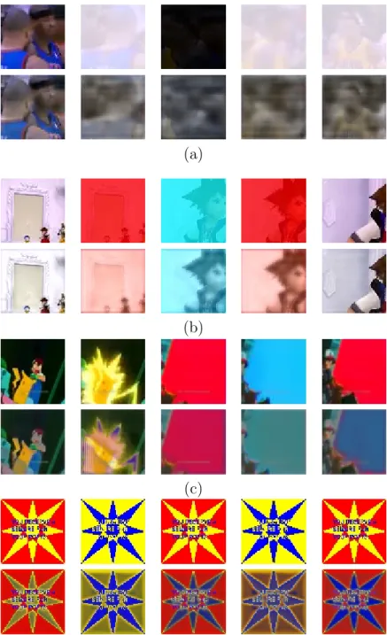
losses and convolution LSTM memory cells . . . 43 4-7 Five frames from 4 videos with their corresponding transformed

versions. Note that frames which are not involved in flashing are preserved while flashes are suppressed in such a way as to not sig-nificantly disturb the underlying contents. Videos (c) and (d) are not synthetic examples created by our generator, (c) having trig-gered hundreds of attacks in children [1] and (d) having been used to target a subject in a politically-motivated attack, causing serious and lasting bodily harm. . . 49 4-8 Conditional Generator for cGAN. 𝑍 refers to the conditional

pa-rameters used to generate the input 𝑉𝑖; ̃︀𝑍 is 64 dimensional latent

vector. . . 50 4-9 Emotion Recognition Discriminator Network . . . 50

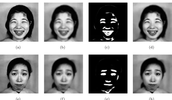
4-10 Output from the GAN generator model. Left: The input sad face to the network. Right: The face transformed to maximize the happy emotion. . . 51 4-11 Top: A highlighted happy face image. Bottom: A highlighted sad

face image. (a,e) are the original source images - 𝐼𝑠. (b,f) are their

blurred counterparts - 𝐼𝑏. (c,g) the learned masks by the sparse

generator model 𝐺* and (d,h) are the output image after applying the mask - 𝐼𝑜 . . . 51

5-1 Website Allowing User to Upload Videos to Demonstrate Network Transformations . . . 55

6-1 GUI for rating images . . . 59 6-2 Human-subject results when asked which video had more flashing

the original or the modified. Subjects overwhelmingly decided that the modified videos had far more flashing regardless of the method introducing that flashing. GANs introduced more subtle flashing of lower frequency. While we do want subjects to choose the generated videos are having more flashing, we do not expect, or desire, that subjects mark the modified videos as entirely consisting of flashes. In other words, the optimal results are not -1 and 1 for the prefer-ence values, because very often the flashes that are problematic are brief and have fairly low intensity. . . 60 6-3 Top: Flash frames output by a GAN. Bottom: Orginal frames. The

GAN learns to insert frames of alternating color into videos with no flashing. In cases where the flashing is of low intensity, the GAN modifies the video to make flashing more pronounced. . . 61

6-4 Comparing the networks on three types of inputs; conditions de-noted by X. The first condition, O, compares against original un-modified inputs where the priority is to keep the stimulus intact meaning we do not desire a preference either way. Similarly, for the next condition, −, where videos were modified to add flashing but with properties that put it below the threshold at which it is likely to cause harm. Finally, + where we see the networks undoing the transformation applied while producing higher quality output and where users prefer their output over the modified videos. Quality is measured as the likelihood of preferring the network output to the output of the condition that is being compared against. Subjects generally judge the quality of the two to be the same, meaning our networks preserve the structure of the videos. . . 62 6-5 Five frames of a black-white flashing video transformed by various

ablated models. Note that frames which are not involved in flashing are usually preserved by all models while attempts are made to suppress flashes in such a way as to not significantly degrade the underlying video content. . . 63

A-1 Unet TensorFlow Graph model. We modified the model to use convolutional LSTMs at its bottleneck. . . 68 A-2 Spatial Temporal TensorFlow Graph model. We modified the model

to use convolutional LSTMs instead of regular LSTMs and remove huber loss penalty. . . 69 A-3 Small convLSTM TensorFlow Graph model. The small network in

chapter 4. . . 70 A-4 Complete Unet TensorFlow graph model (L) and Companion

dis-criminator model (R). A very dense graph that proved challenging to train. . . 71

List of Tables

3.1 Comparison of PEAT and Detector Algorithm on synthetic dataset 27

6.1 Detector results for EpNetSTAE (STAE) trained as a GAN -STAEG - and EpNet-UNET (UNET) . . . 58

Chapter 1

Introduction

Human beings are heavily reliant on visual perception. Of the five senses, sight seems to be the most important. The way we visually perceive the environment greatly affects how we interact with our world. However, even with perfect eye-sight, there are several conditions that may limit visual perception. For example, some individuals with autism may have difficulty perceiving facial expressions. People with photosensitive epilepsy (PSE) may experience adverse reactions, such as seizures and migraines, to certain visual stimuli. Previous work in this domain of assistive technology has mainly focused on how to extract and communicate information from the visual world. Our approach here is to instead transform the visual world to make it more accessible via models that apply arbitrary video-to-video transformations. For this thesis we focus primarily on models with applica-tion in photosensitivity, in the context of photosensitive epilepsy; and secondarily emotion recognition, in the context of the autism spectrum disorder ( ASD), as concrete examples of how this approach can be used in various domains.

Photosensitive epilepsy is a condition that affects 1 in 4000. It is more common in females than males and has higher incidence in children aged 7-19. Those with the condition have adverse reactions to visual stimuli such as strobing lights, spatial oscillations and rapid changes in luminance. Adverse reactions to stimuli range from migraines to severe seizures. With the ever increasing usage of online video streaming, there is a need to detect and filter these problematic stimuli from video content. We develop a tool to create video sequences containing these problematic stimuli, in a way that is likely to arise in real-world videos. We then apply state of the art machine learning models to detect the problematic frames in the generated sequences. We develop more machine learning models to reproduce the video sequences with the problematic frames rendered innocuous.

We find that our machine learning modules are able to reproduce the videos with a substantial reduction in adverse stimuli, rendering most of the videos safe for those with photosensitive epilepsy.

This thesis is organized as follows: In chapters 1 and 2 we motivate and give a brief account of related work on transformative visual assitive technology, paying attention to photosensitivity as our primary application. In chapter 3 we describe some of the features of content that is likely to trigger seizures in photosensitive people and create a dataset of such content. Next, in chapter 4 we describe transformative models with applications in photosensitive epilepsy and autism spectrum disorder that we use to make content more accessible. In chapter 5 we describe how we implement our models and algorithms and explain the design of the codebase. In chapter 6 we report the experimental methods and results used to evaluate our project and conclude in chapter 7.

1.1

Photosensitive Epilepsy

On December 17, 1997 an episode of Pocket Monsters (Pokemon) aired on Japanese television. Approximately 700 people (mostly children) who watched the episode either experienced tonic-clonic seizures or seizure like symptoms related to photo-sensitive epilepsy [2]. Approximately 200 people were admitted to hospital. An official report [3] revealed that around 10% of viewers of the episode experienced various symptoms such as convulsions, loss of consciousness, migraines e.t.c. More than half the seizures were in people who had no previous record of photosensi-tive epilepsy (PSE), thereby highlighting the latent nature of this form of epilepsy. Several studies have shown that a 4 second sequence of frames alternating between long-wavelength red colors and short-wavelength cyan blue colors were likely the offending frames [4]. This is one example that highlights the dangers that video content can pose to people with PSE. Such stimuli have even been used in attacks, defacing the American Epilepsy Foundation website with videos that are crafted to trigger seizures, and in several cases have been involved in politically-motivated attacks against reporters [5, 6] resulting in seizures.

In addition to the Pocket Monsters case, there have been other notable incidents. In the 1980’s, the TV show Captain Powers induced a seizure in a viewer in the US. In 1993 a TV advertisement for Golden Pot noodles was blamed for triggering 3 seizures in viewers in the United Kingdom. [7]. The advertisement had frames with rapid changes in contrast. In 2012, an Olympics Games promotional

video was blamed for triggering seizures in 4 people. More recently, in July 2018, Incredibles 2, the highest-grossing animated feature movie of all time in North America, caused public outcry after it was reported to have caused seizures due to flashing and strobe lights. The Epilepsy Foundation issued a caution to viewers and asked Disney Pixar (the producers of the movie) to post epilepsy warnings on digital properties [8]. Incidents such as these have led to the formation of national guidelines to prevent TV-induced seizures in the United Kingdom and Japan. In the UK the Independent Television Commission (ITC), which now has its duties subsumed by Ofcom [9], developed guidelines to address photosensitive content [10] . The International Telecommunications Union (ITU), which is an agency of the United Nations, also developed a set of guidelines for worldwide content. Similarly, the World Wide Web consortium has guidelines to prevent content that can induce seizures. These are addressed in the Web Content Accessibility Guidelines 2.0 (WCAG 2.0) [11]. In many cases, the guidelines have had several revisions to make them less restrictive and more up to date with scientific knowledge.

The rise of machine learning inference methods over the past decade has produced impressive results in computer vision. Neural Networks, in particular, have proven superior to other methods in tasks such as image object detection and semantic image segmentation. Convolutional neural networks and long short-term memory cells have also proven very effective at extracting high level features from spatial-temporal sequences [12]. We apply this machinery to detect video sequences with problematic stimuli, and render them safe for viewing for those with PSE.

We propose a method to automatically learn filters that are robust with respect to different kinds of patterns, frequencies, and sizes in the field of view. We show three methods to train such video-to-video transformations without specifying or engineering what the transformation should be. First, using an oracle which can take videos and insert harmful stimuli. Second, using a Generative Adversarial Network (GAN) that learns to insert harmful stimuli. And third, using a model for the human visual system which can predict which stimuli are harmful. In each case, a neural network takes as input a short video and learns to transform it into an innocuous video. In the first two cases, the network is trained on videos taken from YouTube, likely not to be particularly problematic, and asked to recover those original videos after they have been augmented to contain problematic stimuli. In the third case, we take as input problematic stimuli and learn to transform them into stimuli that the model for the visual system will consider acceptable. These three methods can be combined together. Critically, they do not specify the transformation, merely the goal of the network in a way that is agnostic about how

it should be achieved. This means the video-to-video network is not tuned in any way to flash mitigation or photosensitive epilepsy. Providing different objective functions can lead to novel kinds of transformations that can help with other accessibility issues.

1.2

Autism

In addition to PSE, we also demonstrate some of the application of these learned transformations in face perception for individuals with some forms of the autism spectrum disorder. Autism spectrum disorder (ASD) is a broad grouping of neu-rodevelopmental disorders that result in deficits in social communication and social interaction, and in restricted repetitive patterns of behavior, interests, and activ-ities [13]. Aspects of face processing and learning have shown disruptions at all stages of development in ASD [14]. Those with this condition risk reduced use of facial information and this may result in an inability to effectively communicate and interact with one’s peers. Unlike PSE, in the case of ASD face perception, the impairment is the result of a deeper neural mechanism and has little to do with the quantitative properties of the visual environment.

Preliminary results from the Stanford Autism Glass Project [15] indicate that highlighting the facial expressions of others can be extremely useful for those with Autism.

We use a neural network adapted from [16] that detects emotions in faces as a proxy for the human visual system. We use this proxy to transform the face images to more strongly convey their emotional content to the visual system.

Chapter 2

Related Work

2.1

Related work

There has been a considerable amount of interest in deep learning sequence-to-sequence models over the past few years. Sequence-to-sequence-to-sequence models have been applied to text, audio and video problems with good results.

For example, sequence-to-sequence models have successfully been used to caption videos [17, 18] and for other video-to-text transformations. Models such as in [19, 20] have been used to recognize actions in videos. Sequence-to-sequence mod-els have been used to increase video resolution by capturing relevant contextual information to interpolate image details. Similarly, they have been applied in the task of coherently fusing multiple video sources without human supervision. Analogously, audio-to-audio transformations have been used to increase audio res-olution [21]. Hall et al. [22] create a model that learns to synthesize speech from text. In robotics, related networks have been used to procedurally generate ob-jects from images to allow robots to learn in simulation and reduce the need for real world training images [23].

More commonly, deep models have been used on image-to-image transformation tasks, and have produced very impressive results. Recent results in style transfer networks show how networks can learn features of style on content separately and can be used to transfer image style from on image to another. Network such as Unet [24], and Segnet [25] have been applied to image segmentation tasks that involve transforming and labelling different segments of the image scene. Con-ditional Generative Adversarial Networks (cGANs) have been used effectively on

tasks such as synthesizing photos from label maps, objects from edge maps, or colorizing photos. Furthermore, methods such as Cycle Generative Adversarial Networks (CycleGANs) have shown how arbitrary image-to-image transforms can be learned in many different domains through the use of adversarial training meth-ods.

Specifically for video-to-video transformations, deep models have been applied in tasks such as optical flow prediction and next frame prediction. In optical flow tasks, the model learns to transform the video frames into flow fields [26]. This is done primarily by inferring future frames generally [12, 27], and in some cases by learning the physics of video scene [28].

Generative models have been widely applied in these tasks as the forward version of these tasks is often simpler and more well defined than the inverse version which can sometimes be ill posed and undefined.

Kulkarni et al. [29] demonstrate how a neural network can recognize faces and disentangle their parameters by learning to de-render and re-render images. Ro-maszko et al. [30] reconstruct 3D scenes from single images using a similar ap-proach. Narayanaswamy et al. [31] reconstruct 3D scenes with occlusion from single images using priors from physics including notions such as stable sup-port. Yuille and Kersten [32] discuss the neural and cognitive plausibility of such analysis-by-synthesis models. The general idea is that analyzing a stimulus re-quires reasoning about the process through which it was created, and that the creation is easier than the analysis, has a long history in both language [33] and vision [34].

These new techniques have not yet been fully explored for their applications to accessibility. Leo et al. [35] provide a thorough and recent review of computer vision for accessibility. A few hand-crafted video-to-video transformations have been considered in the past. Farringdon and Oni [36] record which objects were seen in prior interactions and attempt to cue a user that they have seen those objects before thereby enhancing their memory. Damen et al. [37] build on the prior work and highlight important objects allowing users to discover on their own which objects are useful for which tasks. Betancourt et al. [38] review a rich first-person view literature, focusing on wearable devices that can help with many tasks from navigation to gesture recognition.

Photosensitivity has been recognized as an important concern to broadcast TV for several decades. This led to guidelines limiting the amount of acceptable

flashing [4]. Several tools have been created to detect segments of a video which might be problematic [39–41]. Signal processing has been used to create filters that can eliminate some forms of flashing [42]. Such filters are difficult to create as making problematic stimuli is much easier than detecting them and in turn much easier than repairing them.

Certain types of blue-tinted lenses that filter out short wavelength light have been found to be effective at increasing the threshold at which a stimulus is problem-atic [43]. In this paper, we present the first learned and general-purpose video-to-video transformation to attenuate such stimuli that a user could run on their laptop, phone, television, or in the future, AR glasses, at all times to be passively protected. Moreover, such a transformation can be tuned to individual users, filtering more aggressively for some at the expense of lower visual fidelity when filtering is required.

As was pointed out in the extensive review by Leo et al. [35], computer vision has so far been used to replace particular human abilities by developing algorithms that perform those same tasks and provide users with symbolic information about the environment. For example, commercial systems such as OrCam primarily extract text features, object properties, and face identities from videos and present them in an interactive manner to a user. A few notable exceptions exist. For example, approaches which convert depth maps into auditory cues in order to aid navigation [44]. While not explicitly a video-to-video transformation, Rello and Baeza-Yates [45] present fonts that help those with dyslexia. They do not use computer vision methods but in every other sense they manipulate a visual stimulus to make it more accessible.

This is a significant limitation in the space of assistive technologies that have been considered; many people who could benefit from such technologies, for example the visually impaired, retain part of a sense which can then be augmented. More-over, extracting symbolic information loses part of the richness and texture of the environment in a sense gating perception entirely through the choices of the computer vision system thus depriving users of direct access to the environment. We are not the first to note this or to note that it can be a serious problem in trying to understand one’s surroundings and perform different tasks. In robotics, precisely this problem led to end-to-end learning which has shown that such sym-bolic intermediate representations are very limiting and removing those limitations provides powerful new capabilities. For example, deep reinforcement learning can now learn to play games [46] without human annotations and other work has

shown how robots, again without human annotations, can learn end-to-end poli-cies to carry out different tasks [47]. This would not be possible with the symbolic extract-information-and-use-it approaches. The lessons learned in robotics apply equally in human interactions, and rather than focusing all of our efforts on ex-tracting information and replacing human senses, we believe we should also work on augmenting them. To do so, it is important to learn how one can augment these senses because the transformations that must be performed on a visual or auditory stimulus may not be self-evident. To our knowledge, this is the first work that learns an arbitrary transformation that makes a video accessible for a user.

Chapter 3

Dataset

3.1

Features of Unsafe Videos

There are some differences between the various guidelines on what content is con-sidered unsafe for those with PSE, but there is some consensus, supported by conclusive research evidence, that the following features increase the risk of pho-toic induced seizures particularly if the effect is visible across a substantial portion of the viewer’s field of view (generally > 25% of the screen for standard display sizes). For simplicity, throughout the rest of the paper we will refer to these fea-tures as "flashes" and videos that contain these feafea-tures and are likely to elicit seizures as "unsafe".

1. Saturated red transitions: Red colored flicker at wavelengths of 660-720nm is more likely to provoke seizures than blue or white light of the same intensity [48]. 660-720 nm wavelengths correspond to colors with a red value of close to 255 in the RGB color space. In the PokÃľmon example, it was identified that a sequence of rapid transitions to saturated red color was the major source of seizures. Research by Harding et. al. revealed that color has a major effect on provoking electroencephalogram (EEG) abnormalities [2] which are related to seizure inducing brain activity.

2. Opposing changes in luminance: In the ITU and W3C guidelines, op-posing changes in luminance are restricted. In the W3C guidelines, changes in luminance of more than 10% at more than 3Hz are prohibited. Similarly, in the ITU guideline changes of more than 20𝑐𝑑/𝑚2 _{are prohibited.}

3. High frequency flashes: Flashes at higher than 3Hz have been shown to elicit seizures at a much higher rate than low frequency flashes. The ITU guideline prohibits flashing at greater than 3Hz as does the W3C guideline. Experimental research by Takahashi and Tsukahara [49] found that flicker frequencies in the range 15-20Hz were most effective in eliciting general-ized photoparoxysmal response (PPR) [49] with red flicker stimuli having a greater effect. For our research, we used a threshold of 3Hz to demarcate be-tween high and low frequencies as done in the guidelines. In their research, Fisher et al. [48] showed that flash rates are second only to brightness in their influence over photic or pattern-induced seizures (PPISs) [48]

4. Patterns and Spatial frequency: Some spatial frequencies or patterns, such as alternating parallel lines or stripes, are more likely to provoke PPISs [48]. Work by Binie et. el. shows that grating patterns with alternating changes in direction or phase can be more likely to trigger PPISs. Drifting patterns with 2-4 cycles per degree of view from typical viewing distance can increase the likelihood of PPISs. In their proposal for reviewed ITU guidelines, Wilkins et al. [7] state that potentially harmful patterns are composed of more than five light-dark alternating stripes with the lightest stripe having a luminance of greater than 50𝑐𝑑/𝑚2

5. Area: The area of viewing angle affected by the features above also has an impact on whether the content is likely to elicit PPISs. In most cases an affected area of less than 25% of the screen on a standard television, desktop or laptop is unlikely to provoke seizures. In the W3C and ITU guidelines, flashes that cover less than 25% of the screen are considered safe. Fisher et al. [48] also found that flashes lasting less than half a second are generally safe and unlikely to invoke PPISs.

3.2

Creating Unsafe Videos

Although there is understanding and agreement in the scientific community that the above features make content unsafe, there is no publicly accessible dataset with examples of such content for obvious ethical and safety reasons. In our effort to run machine learning models of such data, we had to synthetically generate a dataset by corrupting videos with flashes.

We downloaded 20,000 random video clips in mp4 format and of resolution higher than 200 x 200 at 30 frames per second of varied duration. Each of these videos was then split into 100-frame chunks thus creating a dataset of 200,412 100 frame chunks. We then pass the chunks through a corruption algorithm defined below.

3.2.1

Corruption Algorithm

This algorithm attempts to corrupt the chunks by adding flashing to a subset of the frames whilst still preserving much of the video content. It aims to generate flashing that can be perceived to arise from natural sources, such as the sun or bright flashing lights, or perturbations in the color space, thus keeping edges intact.

1. For each chunk, we randomly select a duration (seconds) of the flashing from a uniform distribution 𝑑 ∼ 𝑈 (1, 3) and also uniformly select a starting frame for the flash. The effect of provoking PPISs is probabilistic so PPIS frequency increases with prolonged exposure. We determined it is sufficient to keep the duration from 1s to 3s as that is sufficient to elicit PRP and temporal locality in videos makes it unlikely that our machine learning modules would learn useful features for handling the current frame beyond a 3 second window. 2. For each chunk, with 2

6 probability we flag it as a low frequency flash or else flag it as high frequency. The low frequency flashes serve as false positives for our training set where the flash frequency (𝑓 Hz) is drawn uniformly 𝑓 ∼ 𝑈 (1, 3). In the case of high frequency flashes we draw 𝑓 from a trun-cated normal distribution bounded from 15-25Hz and centered at 20Hz i.e 𝑓 sin 𝑁 (𝜇 = 20, 𝜎 = 3, 𝑎 = 15, 𝑏 = 25). In most cases high frequency flashes were rendered at a fixed rate of 15-20Hz regardless of 𝑓 due to limitations imposed by the frame rate. For example, if you alternate between black and white frames at 30FPS, the maximum cycles you can complete in 1 second is 15.

3. Given the values of 𝑑 and 𝑓 we randomly uniformly select a flash type to apply. The flash types are red blue transitions, black white flashes, HSV perturbations, and wavelength distribution shifts. The flash types are detailed in the next section.

3.2.2

Flash types

∙ Red Blue transitions: We modeled these types of flashes closely on the red blue transitions in the PokÃľmon example. In the PokÃľmon example, the offending frames were a sequence of frames with wavelengths alternating from 625nm to 452nm to 704nm [2] with peaks at 625nm and 704nm. To generate similar flashing, we first pick a base color 𝑏 uniformly from 554-700nm 𝑏 ∼ 𝑈 (554, 700) and then produce an alternating sequence of frames with b, b-173nm, b+79nm wavelengths, with the given frequency 𝑓 , after first applying algorithm [50] to convert wavelength to RGB color values. We then sample an alpha value 𝛼 ∼ 𝑁 (𝜇 = 200, 𝜎 = 10) and blend in the flash frames onto the video frames using alpha compositing.

∙ Black-White flashes: This is a type of flashing caused by rapidly alter-nating between light and dark frames to create huge changes in luminance. We simply generate a sequence of alternating frames with white (RGB: 255,255,255) and black (RGB: 0,0,0) at the desired frequency (𝑓 ), then we generate 𝛼 using the same parameters as above and blend in the frames. ∙ HSV perturbations: In this method, we generate flash frames by

modify-ing their values in the HSV color-space. In this way we can simultaneously vary color and brightness values. To generate these flashes we choose the difference between successive flash frames from Gaussian distributions. ∆𝐻 ∼ 𝑁 (𝜇 = 40, 𝜎 = 5)

∆𝑆 ∼ 𝑁 (𝜇 = 30, 𝜎 = 20) ∆𝑉 ∼ 𝑁 (𝜇 = 200, 𝜎 = 50)

∆𝑉 is given a much higher mean because changes in brightness are more effective at provoking PPISs. Unlike previous methods, no alpha compositing is needed as we simply can apply the differentials to alternating frames. The resulting flash frames are more "psychedelic" and closer to many unsafe GIF images that are formed from artificial mixing of bright colors.

∙ Wavelength Distribution shifts: This procedure is a generalized form of the Red Blue flashes we generated above. Rather than fix the peaks as in the Red Blue transitions case, we instead uniformly sample the starting peak 𝑝 ∼ 𝑈 (380𝑛𝑚, 780𝑛𝑚) and then sample the distance to the second peak ∆𝜆 ∼ 𝑁 (𝜇 = 200𝑛𝑚, 𝜎 = 30). Using [50] we convert the peaks to RGB values. This gives two peaks which we use to shift our image distribution

Flash Type Detector PEAT Conv-LSTM Type Freq Status Red3c Red Lum Status Red Lum Status

01 BW L P 6 - - P - - P 02 RB H F 36 37 13 F 34 42 F 03 RB H F 7 27 30 F 44 45 F 04 BW H F 24 - 57 F - 78 F 05 Wav H F 65 32 37 F 66 64 F 06 BW H F 0 R 60 F - 71 F 07 Wav H F 60 61 19 F 58 81 F 08 HSV L P - - - P - - P 09 HSV L P - - - P - - P 10 HSV H F - - 30 F - 75 F 11 RB H F 48 61 39 F 58 61 F 12 Wav L P 10 6 - P - - P 13 BW H F - - 88 F - 88 F 14 BW H F 19 - 49 F - 68 F 15 Wav L P 53 - - P - - P 16 BW H F 52 - 69 F - 64 F 17 BW H F - - 39 F - 46 F 18 Wav H F 96 53 44 F 78 87 F 19 Wav H F 52 42 25 F 37 47 F 20 HSV L P - - - P - - P

Table 3.1: Comparison of PEAT and Detector Algorithm on synthetic dataset

across for successive frames. Again, unlike Red Blue transition we do not use alpha compositing but instead we shift the entire distribution of the frames to be centered on the peaks. This gives flashing where successive frames vary significantly in deep colors.

Tuning

By structuring the corruption algorithm and flash types in this way, we can easily adjust hyperameters to personalize networks towards individual needs. For exam-ple, for individuals sensitive to only extreme forms of adverse stimuli we can use the hyperparameters to reduce 𝜎 and shift 𝜇 towards extreme values. That way, we bias the dataset to only report more extreme flashing images as positive.

Chapter 4

Models

4.1

Detecting flashes

There have been a few attempts to develop flash detection algorithms. The most well known are the Harding FPA tool and the Photosensitive Epilepsy Analysis Tool (PEAT) [51].The Harding FPA tool is a proprietary commercially available tool to analyze seizure risk. PEAT is a freely downloadable tool developed by the University of Maryland. In this section, we describe two methods of detecting flashes in videos. The first is an algorithmic approach that scans the video sequence and analyzes pixel level trends. This works in similar fashion to PEAT. The second is a machine learning model that is trained on the synthetic dataset to learn features of flashing content.

4.1.1

The Detection Algorithm

We use algorithms as described in [52]. A summarized outline of the algorithm is given below:

The first part of the algorithm deals with detecting luminance flashes. To do this we first convert the frames to luminance color space. Then For every frame:

1. Calculate the luminance difference from the previous frame. 2. Compute histograms of positive and negative difference values

3. Scan the histogram bins from highest to lowest until the number of scanned elements is greater than 25% of the frame.

4. Compute the average of the frame by summing bins with a number of el-ements greater than 25% of the frame for both the positive and negative histograms. Take the average with maximum absolute value as the average of the frame.

5. Compare the signs of the previous and current frame. If the signs are equal, the values are added to an accumulator variable. Opposing signs indicate a change in trend and local extreme. We record the value of the local extreme. 6. Using a sliding window, we scan the frames, flagging frames that have more than three local extremes in a 1s window and have local extreme values beyond our threshold 𝐿𝑡ℎ = 20

The second part is detection of saturated red transitions. We use two methods to detect saturated reds transitions. In the first, we check if the mean RGB values of the frame are within bounds we predefined, then we check that the values are within close euclidean distance to 100% saturated red in the 𝑌 𝐶𝑏𝐶𝑟 color

space. 100% saturated red in RGB color space (255,0,0) translates to (76,85,255) in 𝑌 𝐶𝑏𝐶𝑟. For simplicity, we take colors that are within the bounds and with a

euclidean distance less than 90 from (76,85,255) to be saturated reds. If a frame has greater than 25% of its values as saturated reds and there is temporal transition to or from it, from a frame that does not satisfy the saturated red constraints, we flag a saturated red transition. This method is described in detail by Carreira et al. [52]. In the second method, we implement the detector based on specification in WCAG2.0 guideline 2.3. The steps are outlined below.

1. We convert the sequence from RGB to RGB relative luminance as defined

inhttps://www.w3.org/WAI/GL/wiki/Relative_luminance.

2. For each frame we record the change in (R-G-B)x320 as ∆𝐿 setting negative values to 0.

3. If a frame has 𝑅/(𝑅 + 𝐺 + 𝐵) > 0.8 and ∆𝐿 ≥ 20 for greater than 25% of its pixels we flag it for a transition.

4.1.2

Detection Machine Learning Model

Neural networks have proven effective in analysis of video sequences. In particular, convolutional neural networks (CNNs) have proven superior at tasks such as object detection, segmentation and recognition. In combination with long short term memory modules (LSTMs), CNNs can be used to gather image information across a video over longer time periods [53].

For our detection model, we use a neural network model with stacked convolutional layers and rectified linear unit (ReLU) activation, followed by stacked LSTM layers then a single densely connected unit with a binary output signaling whether or not the video has a flash. Our model is based on models discussed in [53] and work on similar models for self driving cars.

4.1.3

Network Architecture

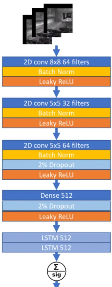
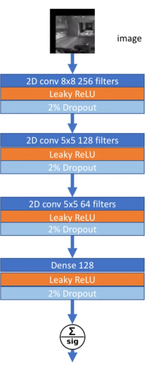
Illustrated in figure4-1, the network architecture consists of first a 8 x 8 time dis-tributed convolution with 64 filters followed by a leaky ReLU activation. We use leaky ReLU units throughout the model to allow for persistent back propagation through the model and prevent the dying ReLU problem. This is especially im-portant when this model is used as a discriminator model for a GAN [54]. Next, we have a 5 x 5 convolution with 32 filters and leaky ReLU activation, then a third time distributed 5 x 5 convolution with 64 filters. All convolutional layers are initialized using He Normal initialization [55]. Next we apply dropout [56] at a rate of 0.2 and Leaky ReLU activation. Dropout adds some noise tolerance to the network and acts as a form of regularization. This is followed by spatially dense fully connected units after which we have more dropout and ReLU activa-tion. To capture time dependent features, we flatten the network both spatially and temporally and connect two densely stacked LSTM layers of 512 units each. Finally, we connect a single dense fully connected unit at the output with sigmoid activation.

We train the network on the synthetic dataset using the binary cross entropy objective function with the Adam [57] optimizer and a learning rate of 10−3.

Figure 4-1: The Detection Model Neural Network

4.1.4

Evaluation of Synthetic dataset, Detection Model and

Algorithm

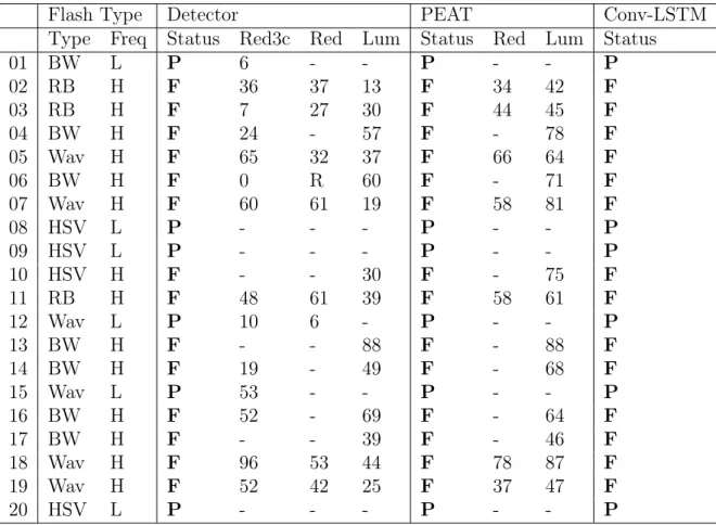
To evaluate our synthetic dataset, we randomly selected a set of 100-frame cor-rupted videos from the synthetic dataset and performed analysis with PEAT. For each video sequence PEAT outputs success if the video is safe and satisfies the W3C Web Content Accessibility Guidelines (WCAG) 2.0 for epileptic content, caution if the video is safe but close to violation, fail if the video violates WCAG 2.0. PEAT has three types of violations: Red flashes, Luminance flashes and Ex-tended flash warnings. In table3.1 we compare the PEAT results vs results from our detector algorithm. For each sample, we list the flash types: Black-White (BW), Red-Blue (RB) , HSV perturbation (HSV), Wavelength shift (Wav) ; and frequency: Low (L) , High (H). For the detector algorithm from 4.1.1 we show whether the sequence passed (P) or failed (F) the safety test. In the correspond-ing columns, we show the count of frames that have red transitions detected uscorrespond-ing our implementation of the detector using W3C WCAG2.0 guideline 2.3 (Red3c), the euclidean distance algorithm (Red) and luminance detector (Lum) from4.1.1. For simplicity, we only show values > 0 if more than 3 flash frames are detected

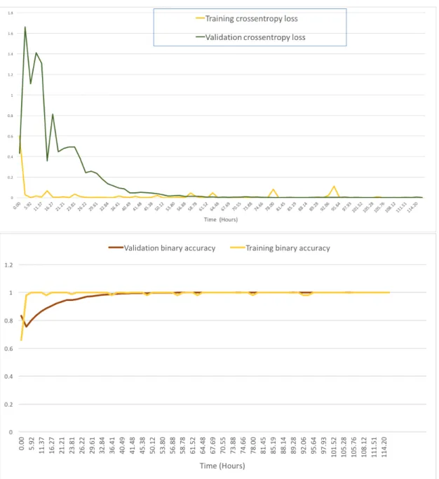
Figure 4-2: Detector network training and validation binary accuracy and crossentropy loss

in a 1s window. In the PEAT column, we show the corresponding count of Red transitions and Luminance flash frames as detected by PEAT and the pass/fail result for the entire sequence. In the final column, we show the status output from the convolutional LSTM neural network (Conv-LSTM) described in 4.1.3.

4.2

Sanitizing Videos

4.2.1

Inverse Pass

The problem of sanitizing videos can be defined as reconstructing an original video 𝑉𝑥 from the corrupted video 𝑉𝑐. Ideally, we want to output a reconstructed video

with as high resolution as the original with most of the flashless frames identical to the original. This is also referred to as the inverse pass, as the objective is to remove added stimuli from the input — a sequence-to-sequence transform.

4.2.2

Regression

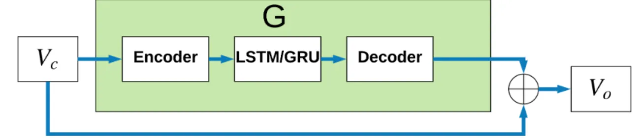
We can formulate this problem as a least squares regression problem where our model takes in as input 𝑉𝑐 and outputs a reconstructed output 𝑉𝑜. As is the case

in most regression problems, the objective is to minimize ||𝑉𝑜− 𝑉𝑥|| by using the

standard mean square error (MSE) as a loss function 𝐿𝑚𝑠𝑒.

Figure 4-3: Video reconstruction.

Encoder-decoder networks used to reconstruct videos without adverse stimuli. LSTM cells are placed in between the encoder and decoder modules.

We created several deep network models to test on this regression model. We drew inspiration of design of the models from [12] and [58]. Patraucean et al. [12] show that encoder-decoder networks in combination with LSTMs can be used to predict the next frame optical flow and are effective at capturing spatial and temporal features. Ronneberger et al. [58] describe the design of Unet. Unet is a widely used encoder-decoder network for segmentation and is also capable of capturing high resolution features by its use of skip connections between encoder and decoder layers. Our models have one major pathway that is used to learn a residual. Let 𝐺 represent this residual pathway. Then:

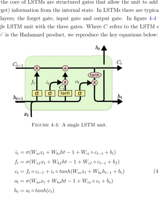
Traditional recurrent networks have trouble picking up long term dependencies. For our problem, adverse stimuli (flashes), may span substantial portions of the 100-frame sequence, as such long term dependencies are critical to resolving the subsequent frames after long periods of flashing. For example, if we have a sequence of black-white flashing spanning 40 frames on a 100 frame video, the brightness of the flashing frames maybe so severe that in order to restore the flashing frames we may have to look back more than 30 frames. LSTMs [59] have shown to be able to capture long term dependencies and have shown great results on sequence-to-sequence problems, music composition[60], handwriting recognition [61] and many others. At the core of LSTMs are structured gates that allow the unit to add or remove (forget) information from the internal state. In LSTMs there are typically three gate layers; the forget gate, input gate and output gate. In figure 4-4 we show a single LSTM unit with the three gates. Where 𝐶 refers to the LSTM cell state and ’∘’ is the Hadamard product, we reproduce the key equations below:

Figure 4-4: A single LSTM unit.

𝑖𝑡= 𝜎(𝑊𝑥𝑖𝑥𝑡+ 𝑊ℎ𝑖ℎ𝑡 − 1 + 𝑊𝑐𝑖∘ 𝑐𝑡−1+ 𝑏𝑖) 𝑓𝑡= 𝜎(𝑊𝑥𝑓𝑥𝑡+ 𝑊ℎ𝑓ℎ𝑡 − 1 + 𝑊𝑐𝑓 ∘ 𝑐𝑡−1+ 𝑏𝑓) 𝑐𝑡= 𝑓𝑡∘ 𝑐𝑡−1+ 𝑖𝑡∘ 𝑡𝑎𝑛ℎ(𝑊𝑥𝑐𝑥𝑡+ 𝑊ℎ𝑐ℎ𝑡−1+ 𝑏𝑐) 𝑜𝑡= 𝜎(𝑊𝑥𝑜𝑥𝑡+ 𝑊ℎ𝑜ℎ𝑡 − 1 + 𝑊𝑐𝑜∘ 𝑐𝑡+ 𝑏𝑜) ℎ𝑡= 𝑜𝑡∘ 𝑡𝑎𝑛ℎ(𝑐𝑡) (4.2)

We use convolutional LSTMs as defined in [62]. These are LSTM layers that make use of the convolutional operation to capture spatial information and thus reduce the number of parameters analogous to convolutional networks and fully connected networks. In the convlutional LSTM architecture, the cell outputs, its

hidden state and gates are instead 3D tensors where the last two dimensions are spatial (row and columns) [62]. The modified key equations from [62] for the convlutional LSTM are reproduced below where * is the convolutional operator:

𝑖𝑡= 𝜎(𝑊𝑥𝑖* 𝑥𝑡+ 𝑊ℎ𝑖* ℎ𝑡 − 1 + 𝑊𝑐𝑖∘ 𝑐𝑡−1+ 𝑏𝑖) 𝑓𝑡= 𝜎(𝑊𝑥𝑓 * 𝑥𝑡+ 𝑊ℎ𝑓 * ℎ𝑡 − 1 + 𝑊𝑐𝑓 ∘ 𝑐𝑡−1+ 𝑏𝑓) 𝑐𝑡= 𝑓𝑡∘ 𝑐𝑡−1+ 𝑖𝑡∘ 𝑡𝑎𝑛ℎ(𝑊𝑥𝑐* 𝑥𝑡+ 𝑊ℎ𝑐* ℎ𝑡−1+ 𝑏𝑐) 𝑜𝑡= 𝜎(𝑊𝑥𝑜* 𝑥𝑡+ 𝑊ℎ𝑜* ℎ𝑡 − 1 + 𝑊𝑐𝑜∘ 𝑐𝑡+ 𝑏𝑜) ℎ𝑡= 𝑜𝑡∘ 𝑡𝑎𝑛ℎ(𝑐𝑡) (4.3)

The design of convolutional LSTMs reduces the number of training parameters. However, due to the long term dependencies to be learned, training convolutional LSTMs is still considerably more difficult than 2D convolutional networks. Fur-thermore, in most machine learning frameworks, such as TensorFlow, the LSTM units are first unrolled in time, thus consuming considerable amounts of memory.

4.2.3

Models

Some of the models we experimented with are described below. The input to each model is the 100 frame 64x64 video corrupted video 𝑉𝑐 in RGB color space, scaled

and shifted to fit its values in [-1,1]. This transformation helps learning because of alternating gradients and because 0 is the default padding value. The target to the models is 𝑉𝑥 scaled in the same way. For most models, we generally use

small convolutional kernels with stride=1 to allow for greater depth and improved performance as shown in VGG [63]. Unless otherwise stated, we use Xavier Glorot initialization [64] for the convolutional layers.

∙ smLSTM: A relatively very small network. The first layer is a 4x4 con-volution with 4 filters activated by ReLU, followed by batch normalization [65]. In testing we found batch normalization generally accelerates learn-ing. In the next layer we include a 3x3 convolutional LSTM. We make this layer bidirectional by passing the sequence forwards and backwards in time. The final layer is a 3x3 convolutional layer with 3 filters (one of each color channel). This layer has no activation function and its output is the learned residual. Our motivation for this approach was to quickly test the types of flashing a simple network would be capable of handling. We quickly found

that this network was able to address flashing caused by saturated reds after only a few training steps

∙ STA: This network is largely based on the spatial temporal encoder in [12] used for optical flow generation. The first 4 layers are 32 filter convolutional layers with 3x3 kernels and ReLU activation. Next there is one layer of pooling to complete the encoder section. Following this, we insert two 32-filter convolutional LSTM layers, followed by two regular convolutions with large 15x15 kernels. After this we have a 2-filter 1x1 convolution and a 2-filter 3x3 convolution. Patraucean et al. [12] explain that they use large 15x15 kernels to "regress from the memory feature space to the space of flow vectors". We can relate our problem to that of optical flow by casting our problem as next frame prediction following the beginning of a flash. Therefore, the extracted optical flow features can similarly be effective for video sanitization. Unlike [12] we did not apply a Huber loss penalty. The encoder portion of this network is the inverse of the decoder. This network was relatively wide and deep. Our primary motivation for this approach was to see if a network of stacked layers was capable of video reconstruction in similar fashion to optical flow prediction. A subtle difference between this network and smLSTM is that we do not use bidirectional LSTMs, so next frame prediction is based on previous frames.

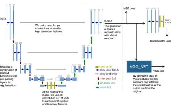
∙ Unet: The Unet architecture [58] has been widely successful on image seg-mentation tasks. Unet works by first encoding the input image to a lower spatial dimensional embedding, through a contracting path, then decod-ing that embedddecod-ing into a segmentation map. The central idea is that the network learns a lower dimensional embedding that captures the semantic details of the images. Unet makes use of dropout and spatial dimensional reduction for regularization. To capture high resolution features, Unet has many skip connections between the encoder layers and their corresponding decoder layers. This allows Unet to output very high resolution images even after contracting the spatial dimensions in the encoder step.

We took the official Unet [58] and modified it to include convolution LSTM units between the encoder and decoder. We stacked 4 convolutional LSTM layers with 64,32,32 and 64 filters respectively between the encoder and de-coder. All layers used small 3x3 kernels. Each LSTM layer was wrapped with a bidirectional feeder that feeds the LSTM both the forwards and backwards versions of the sequence. This network is significantly larger and deeper than

previous networks described. In figure 4-6 we give a schematic of the modi-fied unet network.

4.2.4

Issues

We found deeper models to be particularly difficult to train. Two main problems we faced were regression to mean and regression to identity. The heart of these problems lies in using MSE as an objective function. MSE is ill suited for this problem as it does not account for semantic details. Without properly capturing semantic details, there can be degradation in the autoencoder and loss of high resolution details. Unet mitigates this loss by using many skip connections; networks such as [12] impose a smoothness penalty across successive frames. In the first problem, regression to mean, we found that our deeper networks would address flashing by blurring in the surrounding flash frames. In some cases, the network would simply learn to apply a low luminance color haze across the sequence. This would address flashing and lead to a lower average squared error in RGB color space but would lead to a significantly modified sequence even if the input sequences had no flashing at all. In the next section, we explain some adjustments we make to the objective function that address this problem.

Another problem we faced was regression to the identity function; Because of sparsity in the flash frames, the identity function has a very low MSE. In this case, the network would simply learn the identity function. This regression to the identity function was particularly prevalent in our deeper models that lacked sufficient regularization. This prompted our initial decision to use small 100 frame-sequences at 30 FPS (3 second videos) to reduce the fraction of flash-free frames and avoid biasing the network towards identity.

4.2.5

Attention

Recent works such as [66], [67] and [68] show how attention models can successfully be used in conjunction with recurrent models for sequence-to-sequence transduc-tion and spatial transformatransduc-tion problems. In fact, in [66], the authors show how attentive mechanisms can be used entirely in place of recurrent networks. They also show how attention mechanism can be used to speed up training time and build models that are easily parallelizable and improve performance. Mnih et al.

[67] show how attention-based models can be better at dealing with clutter and scale better to large images [67].

Much of the earlier work on attention based models was inspired by human percep-tion. Humans do not process an entire scene at once, instead humans selectively choose portions of a scene to process at a time, paying particular attention to por-tions of interest, then gather information from across these different porpor-tions of the screen to process the scene. By combining this information over time humans build up an internal representation of the scene, guiding future eye movements and decision making [67]. In humans, this in turn reduces complexity and allows our perception to scale as we can ignore regions of less importance, or parts of the scene that contain visual clutter and instead devote more attention towards objects of interest in the scene.

We can reframe our transformation model as an attentive model that pays atten-tion to poratten-tions of the frames containing adverse stimuli and transforms them. In particular, we can perform soft attention in conjunction with our LSTM mem-ory cells and 2D convolutions to create models that perform attention and are differentiable. We apply similar ideas to this in section 4.3.

As defined in [66], an attention function can be described as mapping a query and a set of key-value pairs to an output, where the query, keys, values, and output are all vectors. The output is computed as a weighted sum of the values, where the weight assigned to each value is computed by a compatibility function of the query with the corresponding key. Thus, our transformative models as discussed above and illustrated in figure4-3 function as a form of additive attention by using 𝐺 to attend to parts of the image with flashing. Observe that for pixel 𝑝𝑖,𝑗 in 𝑉𝑐, the

network learns 𝐺(𝑉𝑐)𝑖,𝑗 = 0 if pixel 𝑝𝑖,𝑗 is not involved in flashing and 𝐺(𝑉𝑐)𝑖,𝑗 ̸= 0

if 𝑝𝑖,𝑗 belongs to a flashing region. In this sense, the attentive key value pairs

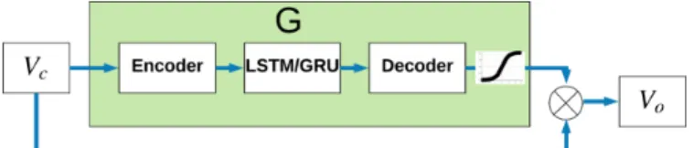
are from the image pixels and the generator learns to query the keys for flashing regions. Instead of additive attention we can also use element-wise multiplicative attention. In this case, we apply tanh activation on the output of the decoder and perform element-wise multiplication with the input to remove flashing regions. In this case the network learns 𝐺(𝑉𝑐)𝑖,𝑗 = 1 if 𝑝𝑖,𝑗 is flashing. The output of the model

is now:

Figure 4-5: Video reconstruction with simple elementwise multiplicative at-tention

In practice we find element-wise multiplication works better as the tanh activation keeps the decoder output in the range -1 to 1; this makes the network train faster and allows for regions not containing adverse stimuli to be easily ignored by setting tanh to the saturated region to output 1. Of course, this simple multiplication is very different from the more complex attentive mechanisms in literature and does not fit the definition of soft attention, but the underlying concept behind it is the same. In future, we can reconstruct our model to use a soft attention mechanism as defined in literature and would expect to see improved performance.

4.2.6

Generative Adversarial Networks

We can use Generative Adversarial Networks (GANs) [69] to generate sanitized videos from the corrupted versions. Works by [70] [71] have shown how GAN can be used to effectively fill in corrupted or missing sections of images. [72] show how discriminator generator Deep Convolutional GANs (DCGANs) can be used for super-resolution, denoising and debluring. The principal idea behind GANs is that a generative model can be trained by splitting it into two components: 1. The generator, such as the models in section4.2.3, whose job is to generate values. 2. The discriminator, such as the model in section 4.1.3, whose job is to classify the generated values. In GANs both components are set up in adversarial fashion such that each component is pushing the other for better performance.

The traditional GAN learns a mapping from a random distribution 𝑧 ∼ 𝑝𝑧 to a

target distribution 𝑥 ∼ 𝑝𝑑𝑎𝑡𝑎with the Generator (G) being the model to learn the

mapping 𝑔 : 𝑧 −→ 𝑥. The discriminator learns to distinguish between the real and generated images. By training the discriminator and generator in tandem the re-sulting generative distribution moves closer to the real distribution 𝑝𝑑𝑎𝑡𝑎. Formally,

D and G play an adversarial min-max game with value function 𝑉 (𝐺, 𝐷)[69] : 𝑚𝑖𝑛

The GAN training algorithm from [69] is: for number of training iterations do

for k steps do

Sample minibatch of 𝑚 input examples 𝑧 ∼ 𝑝𝑧

Sample minibatch of 𝑚 examples from target distribution 𝑥 ∼ 𝑝𝑑𝑎𝑡𝑎

Update the discriminator by stochastic gradient ascent where 𝜃𝑑 are the

discriminator parameters: ∇𝜃𝑑 1 𝑚 ∑︀𝑚 𝑖=1 [︃ 𝑙𝑜𝑔𝐷(𝑥(𝑖)_{+ 𝑙𝑜𝑔((1 − 𝐷(𝐺(𝑧}(𝑖)₎₎₎ ]︃ end

Sample minibatch of 𝑚 input examples 𝑧 ∼ 𝑝𝑧

Update the generator by stochastic gradient descent where 𝜃𝑔 are the

generator parameters: ∇𝜃𝑔 1 𝑚 ∑︀𝑚 𝑖=1𝑙𝑜𝑔((1 − 𝐷(𝐺(𝑧 (𝑖)₎₎₎ end

Algorithm 1: Training A GAN

A caveat of adversarial networks is that the training can be highly unstable, re-sulting in generators that produce nonsensical output [54,73]. In addition to mod-ifying the objective function, we use additional techniques from literature such as adding noise and flipping labels to attempt to improve stability of the networks. However, even with those additions the GANs were unstable and we are yet to develop a more principled approach to the training procedure. Improving stability of GANs is an ongoing area of research in the machine learning community.

4.2.7

Objective Loss

A major problem with using MSE of 𝑉𝑥 and 𝑉𝑜 (𝐿𝑚𝑠𝑒) as an objective loss function

is that the output may lack high frequency details. It may lead to a resulting video where flashing frames are smoothed out and lack detail. Wu et al. [74] show how GANs in combination with with perceptual loss can be used to improve results in image super-resolution. Minimizing perceptual loss leads to images that are more visually pleasing. We first experiment with incorporating perceptual loss in our regression model from4.2.2. A common method of perceptual loss in image super-resolution is to use the higher level features of an imagenet pretrained VGG net as described in [75]. This works well for image-resolution as the features learned by VGG contain semantic representations of images. The VGG perceptual loss 𝐿𝑣𝑔𝑔 is defined as the MSE between the target and input at the output of the 5th

VGG-16 pooling layer. However, for our purposes VGG is not solely sufficient as the pretrained VGG does not learn temporal features. To further improve our model, we can also use a pretrained detector network from4.1.3as a discriminator network to the model and incorporate the discriminator output into the objective loss. In our setup, the output of the discriminator is the confidence of a detected flash. Its loss is the binary crossentropy 𝐿𝑑 from the target label 𝑡 (𝑡 = 1 if the

input video contains a flash) This is precisely what our generative model is trying to minimize. Let 𝐷 represent the function learned by that discriminator, and 𝑉 𝐺𝐺 the VGG-16 function up to the 5th pooling layer. We can define our total loss as a combination of the perceptual loss, discriminator crossentropy and MSE; given weights 𝛼, 𝛽, 𝛾

𝐿𝑑= (1 − 𝑡) · 𝐿𝑜𝑔𝐷(𝑉𝑜) + 𝑡 · 𝐿𝑜𝑔(1 − 𝐷(𝑉𝑜))

𝐿𝑣𝑔𝑔 = 𝑎𝑣𝑔(||𝑉 𝐺𝐺(𝑉𝑜) − 𝑉 𝐺𝐺(𝑉𝑥)||2)

𝐿𝑡𝑜𝑡𝑎𝑙= 𝛼 · 𝐿𝑚𝑠𝑒+ 𝛽 · 𝐿𝑑+ 𝛾 · 𝐿𝑣𝑔𝑔

(4.6)

This setup is similar to a DC-GAN, except in this case, the discriminator (D) is fully trained beforehand rather than in adversarial fashion. Thus, in this case 𝐿𝑑 would essentially function as the adversarial loss. The essential difference is

that in GANs we alternatively train the generator (G) and D rather than rely on pretrained weights. In our GAN setup G is simply one of the models from section 4.2.3. In figure 4-6 we show a modified version of the Unet architecture that supports these additional losses.

In Chapter 4-7(c) and (d) we show frames from videos which are known to have caused hundreds of hospital visits that could have been prevented with this ap-proach. Note that the transformed frames are significantly clearer and easier to understand.

As described in section 2.1, there are some existing specifications for what content is likely to trigger a seizure based on changes in luminance and other properties of the images. We used this information as a basis for developing the corruption algorithm for the dataset and for the hand detector algorithms in chapter 3. Sim-ilarly, we can construct an oracle based on these specifications that is capable of serving as a discriminator network. Of course, this oracle would be insufficient on its own to serve as a discriminator as it would have no trainable parameters and the generator would simply learn to fool the oracle with low luminance images or garbage. However, in collaboration with other loss functions and elements of trainable discriminators, the output from the oracle can be effective at guiding

Figure 4-6: The Unet encoder-decoder network modified to support additional losses and convolution LSTM memory cells

the model towards a more optimal solution more quickly. To construct this oracle we engineered parts of the hand detector to use differentiable tensor ops. This is essential as it allows back propagation through the oracle to the generator. We build two subnetworks: one to detect luminance flashes and another to detect saturated reds. Given an rgb-to-relative luminance weight matrix 𝑊𝑟2𝑙 as defined

in the W3C guidelines, we can use a series of tensor ops and convolutions to ap-proximate the count of flashing frames in a video 𝑥 where * is the convolution operator: 𝑊𝑟2𝑙 = [︁ 299.0 1000 587.0 1000 114.0 1000 ]︁

Result: Count of luminance flashing frames; 𝑥𝑙 ← 𝐴𝑣𝑒𝑟𝑎𝑔𝑒𝑃 𝑜𝑜𝑙(𝑥 · 𝑊𝑟2𝑙) 𝑥𝑝𝑜𝑠 ← 𝑅𝑒𝐿𝑈 (|∇𝑥𝑙| − 20) 𝑥𝑝𝑜𝑠 ← 2 · (𝜎(𝑥𝑝𝑜𝑠) −1 2) 𝑥𝑝𝑜𝑠 ← 𝑅𝑒𝐿𝑈 (𝑥𝑝𝑜𝑠) 𝑐𝑜𝑢𝑛𝑡 ← [[𝑥𝑝𝑜𝑠 * 𝑊𝑐𝑜𝑛𝑣 > 𝑡ℎ]]

Algorithm 2: Luminance Flash Detection Tensor Graph Ops.

𝑊𝑐𝑜𝑛𝑣 is a fixed 30-frame kernel to detect flashes analogous to the sobel filter for

𝑊𝑐𝑜𝑛𝑣 to all ones will simply count the number of positive differentials in a

30-frame window (1s) which in itself is a useful metric to count flashing 30-frames. 𝑡ℎ is the threshold bias for how much flashing frames to allow in the 1s window. Result: Count of saturated red frames;

𝑥𝑟 ← 𝑥 255.0 𝑥𝑟[< 0.0392] ← 𝑥𝑟[< 0.0392] 12.92 𝑥𝑟[> 0.0392] ←(︁𝑥𝑟[> 0.0392] + 0.055 1.055 )︁2 𝑅, 𝐺, 𝐵 ← 𝑠𝑝𝑙𝑖𝑡(𝑥𝑟) 𝑓 𝑟𝑎𝑐 ← 𝑅 𝑅 + 𝐺 + 𝐵 + 𝜖) 𝑥𝑟𝑒𝑑 ← 𝑟𝑒𝑑𝑢𝑐𝑒_𝑚𝑒𝑎𝑛(𝑥𝑟[𝑓 𝑟𝑎𝑐 > 0.8 & ∇𝑥𝑟 > 20]) 𝑐𝑜𝑢𝑛𝑡 ← [[𝑥𝑟𝑒𝑑 * 𝑊𝑐𝑜𝑛𝑣> 𝑡ℎ]]

Algorithm 3: Red Flash Detection Tensor Graph Ops.

We use a similar strategy to develop the oracle for saturated red detection, as shown in algorithm 3. We first convert the RGB image to sRGB space then to relative luminance space as defined in the W3C guidelines. Next, for each frame pixel we calculate its fraction of the red component and its gradient. We then select regions that have greater than 80% red component and have a gradient greater than 20. By passing another sliding window over these regions we can count how many saturated regions we have in a 1s window. This gives a reasonable estimate of the saturated red regions in a video.

We can then use these values to improve our discriminator loss. Where 𝐿𝑙𝑢𝑚 is

the average of the output counts from the oracle we modify our total loss from equation 4.6 to be:

𝐿𝑡𝑜𝑡𝑎𝑙 = 𝛼 · 𝐿𝑚𝑠𝑒+ 𝛽 · 𝐿𝑑+ 𝛾 · 𝐿𝑣𝑔𝑔+ 𝜁𝐿𝑙𝑢𝑚 (4.7)

In testing, we found that including this loss led to networks quickly learning to blur out flashing regions. Due to computational complexity, we rarely tested models that used all components of the loss function. In most cases we trained the model only using two losses i.e usually two of 𝛼 , 𝛽, 𝛾 , 𝜁 were set to 0.

4.2.8

Forward Pass

We apply these models to the forward pass in addition to the hand algorithm from chapter 3. By forward pass, we are referring to the process of synthesizing adverse

stimuli in the case of PSE. In the more general case, for assistive technology this would refer to the process of producing content with inaccessible components. For example, components of an audio recording could be suppressed to synthesize data that is inaccessible to those audibly impaired. Generally, the forward pass is easier to specify and implement as the conditions are typically well understood. For example, in the case of PSE it is well understood that likelihood of adverse flashing stimuli triggering a seizure is a function of its frequency, intensity, field of view and wavelength as described in chapter 3. For many problems of this nature, there is limited real-world data. The key point of the forward pass is that we are able to generate enough data to augment the real-world data, and that by being able to control how this data is generated we guide the behavior of models that train on this dataset.

To synthesize this data we can manually run the algorithm from chapter 3. We take care to insert stimuli both above and below the threshold at which they are problematic. We can also generate the data automatically using the models in section 4.2.3 as GANs. Specifically, we use conditional GAN networks [76, 77] to train a GAN over the already manually generated synthetic examples to generate more examples with adverse stimuli. Isola et al. [77] show how conditional GANs can be used for a variety of image-to-image generation tasks. In figure 4-8 we illustrate a conditional setup for the generative model of the adversarial network. This setup is similar to the traditional GAN generator except we introduce a conditional variable 𝑍 which we concatenate to the input to the generator. In similar fashion to [77] we only condition on the generator and do not directly add any noise to the input. Instead we introduce some noise by sampling a latent vector

̃︀

𝑍 from 𝑍. The input to the generator is the video 𝑉𝑖, and the parameters used

to generate its synthesized counterpart (which is the target of the model) are fed into 𝑍. These parameters include the type of flashing, its duration and frequency as specified in section 3.2.1. Using 64 unit dense layers we reparameterize 𝑍 to intermediate mean and variance vectors which we then use to normally sample

̃︀

𝑍. We apply KullbackâĂŞLeibler divergence from the normal distribution as a regularization penalty term to ̃︀𝑍. In figure 6-3we show examples of frames output for the cGAN. We observed that for video with low intensity flashing the network would amplify the flashing intensity and frequency. Like in [77], our trained model was very deterministic.

4.3

Emotion Recognition

Another example application of our image transformations, is the recognition of facial emotions as described in section 1.2 of Chapter 1. We develop image trans-formation networks able to recognize emotions and apply the desired transforma-tions.

Work by Levi and Hassner [78] has shown how convolutional neural networks can be effective at detecting faces and recognizing emotions from images. In [16], the authors describe models that are effective at recognizing emotion from images. These are networks that can perform inference very quickly and demonstrate the feasibility of implementing neural networks in real-time to detect human emotions [16]. In emotion recognition, humans are able to generally identify most emotions by looking only at few parts of the face (mostly the eyes and lips). An interesting fact is that the emotions happiness, sadness, fear, anger, disgust, contempt and surprise are universally recognizable regardless of one’s cultural background [16] [79]. Image transformation networks that are able to learn these features and either highlight or make them more salient would be beneficial for individuals with certain forms of autism as described in section 1.2. We attempt to create such networks. This general approach to learning could also be beneficial to those with low vision or other impairments that make emotion recognition challenging. In this application, neural networks serve more closely as a proxy for the human visual perception system. It has been shown that convolutional neural networks seem to approximate part of the human visual system [80].

4.3.1

Dataset

To develop our transformative models, we use images selected from the Japanese Female Facial Expression (JAFFE) database [81]. This database consists of grayscale images of Japanese female faces taken in laboratory conditions. Subjects were asked to display 7 facial emotions (6 basic emotions + 1 neutral). Each of the im-ages is then rated by a panel of 60 subjects. For most of our purposes we simply considered the happy and sad emotions. To expand the dataset, we applied sev-eral transformations such as random scalings, flips and rotations on the fly during training. This helps to reduce overfitting during training.