Deep Mining : scaling Bayesian auto-tuning of data science pipelines

(1)

Deep Mining: Scaling Bayesian Auto-tuning of Data

Science Pipelines

by

Alec W. Anderson

S.B., Massachusetts Institute of Technology (2017)

Submitted to the Department of Electrical Engineering and Computer

Science

in partial fulfillment of the requirements for the degree of

Master of Engineering in Electrical Engineering and Computer Science

at the

MASSACHUSETTS INSTITUTE OF TECHNOLOGY

September 2017

c

○ Massachusetts Institute of Technology 2017. All rights reserved.

Author . . . .

Department of Electrical Engineering and Computer Science

August 14, 2017

Certified by . . . .

Kalyan Veeramachaneni

Principal Research Scientist

Thesis Supervisor

Accepted by . . . .

Christopher J. Terman

Chairman, Masters of Engineering Thesis Committee

(2)

(3)

Deep Mining: Scaling Bayesian Auto-tuning of Data Science

Pipelines

by

Alec W. Anderson

Submitted to the Department of Electrical Engineering and Computer Science on August 14, 2017, in partial fulfillment of the

requirements for the degree of

Master of Engineering in Electrical Engineering and Computer Science

Abstract

Within the automated machine learning movement, hyperparameter optimization has emerged as a particular focus. Researchers have introduced various search algorithms and open-source systems in order to automatically explore the hyperparameter space of machine learning methods. While these approaches have been effective, they also display significant shortcomings that limit their applicability to realistic data science pipelines and datasets.

In this thesis, we propose an alternative theoretical and implementational ap-proach by incorporating sampling techniques and building an end-to-end automation system, Deep Mining. We explore the application of the Bag of Little Bootstraps to the scoring statistics of pipelines, describe substantial asymptotic complexity improve-ments from its use, and empirically demonstrate its suitability for machine learning applications. The Deep Mining system combines a standardized approach to pipeline composition, a parallelized system for pipeline computation, and clear abstractions for incorporating realistic datasets and methods to provide hyperparameter optimization at scale.

Thesis Supervisor: Kalyan Veeramachaneni Title: Principal Research Scientist

(4)

(5)

Acknowledgments

I would like to thank my adviser, Kalyan Veeramachaneni. His feedback and ideas made this work possible, and his vision and passion guided me throughout this work.

I’d also like to thank my DAI labmates and the Feature Labs team for their helpful feedback and company.

I’d like to thank my friends for all of their support over the last four years and for making my MIT experience very special. The ideas and support you gave me

continued to push me, and I couldn’t have done it without you.

Finally, I’d like to thank my mom, my dad, and my brother. Words can’t express

(6)

(7)

8.1.5 Custom Pipeline Example . . . 83 9 Experimental Results 87 9.1 Datasets . . . 87 9.1.1 Handwritten Digits . . . 87 9.1.2 Sentiment Analysis . . . 88 9.2 Pipelines . . . 88 9.3 Methodology . . . 90 9.4 Evaluation . . . 90 9.4.1 MNIST Dataset . . . 91 9.4.2 Text Dataset . . . 91 9.5 Results . . . 91 9.6 Discussion . . . 94 10 Conclusion 97 10.1 Future Work . . . 97

A Comments on Apache Spark 99

(10)

(11)

List of Figures

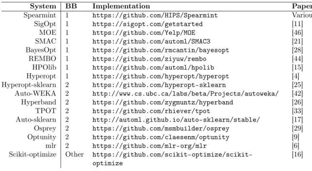
1-1 End-to-end pipeline to build a predictive model. It includes the

pre-processing and feature extraction steps along with the modeling steps. 17

2-1 Illustration of the first common abstraction approach. The optimiza-tion algorithm gives hyperparameter sets to and gets performance

met-rics from the pipeline, which it treats as a black box. . . 29

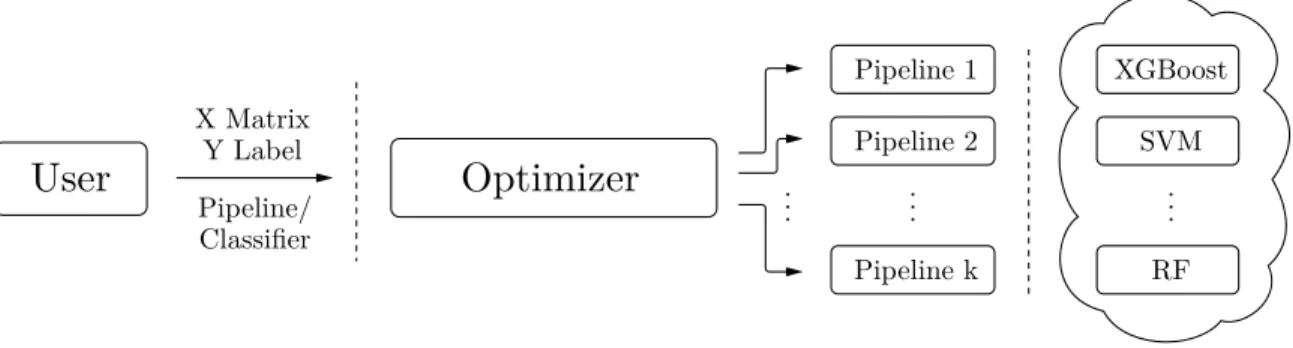
2-2 Illustration of the second common abstraction approach. The user

provides data in a matrix format (either 𝑋, 𝑌 , or 𝑋 and 𝑌 in a cross

validation split). The optimizer chooses a pipeline from within its implemented machine learning algorithms, and returns a classifier or

pipeline with the highest score to the user. . . 29

(12)

3-2 Illustration of the Deep Mining system’s functionality. The user spec-ifies a pipeline using the provided framework, providing

hyperparam-eter ranges and the necessary pipeline steps to the pipeline construc-tor and execuconstruc-tor. The user also provides the data in either raw or

matrix format and cross-validation parameters to the data loader as well as optimization parameters to the Bayesian optimizer. Outside

of the user’s view, Deep Mining constructs a scoring function using the provided pipeline and parameters, incorporating distribution and

sampling to accelerate the evaluation process. Deep Mining also loads the data into a cross validation split for the pipeline executor, which

chooses between different parallel and non-parallel evaluation methods that return a score to the pipeline executor. The Bayesian optimizer

interfaces with the pipeline executor, suggesting hyperparameter sets to evaluate given scores for previous sets. Within the Bayesian

opti-mizer, the Smart Search algorithm provides previous hyperparameters 𝐻 and associated scores 𝑔(ℎ) to the GP or GCP model, receiving an

estimate ˆ𝑔(ℎ) of the scoring function in return. Finally, the pipeline executor returns the tuned pipeline and (optionally) tested

hyperpa-rameters and associated performances. In this figure, the labels are as follows: (1) corresponds to the hyperparameter ranges; (2) to the

(custom) pipeline steps; (3) to the tested hyperparameters and asso-ciated performances; (4) to the pipeline with the best hyperparameter

set; and “P + D + Params” to the scikit-learn Pipeline object, data,

and BLB hyperparameters. . . 36

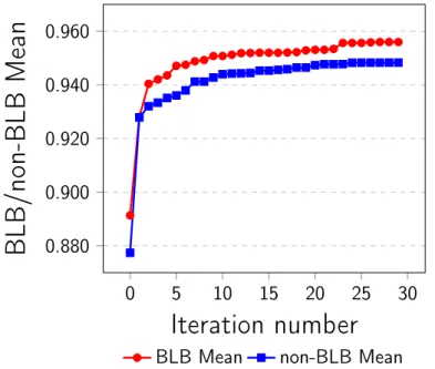
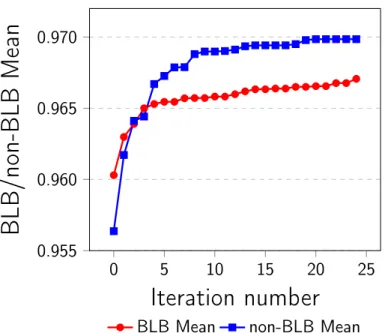
9-1 Experimental averages for the HOG image pipeline. . . 92

9-2 Experimental averages for the CNN Image pipeline. . . 93

(13)

List of Tables

2.1 (Approximate) Classification of current state-of-art Hyperparameter

Systems. BB refers to the type of api or the black box function

method they use. BB= 1 implies that the api is as shown in Figure 2-1

and BB= 2 implies that the system has api as shown in Figure 2-2. . 28

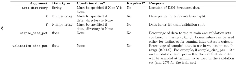
8.1 Arguments for d3m_load_data function. . . 79

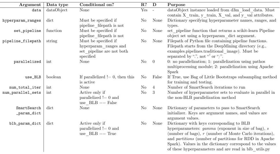
8.2 Arguments for DeepMine function. R= Required?, D = Default . . . 81

9.1 Types of pipelines. . . 89

9.2 BLB and non-BLB processes statistic. . . 94

B.1 Deep Mining Functions . . . 102

(14)

(15)

Chapter 1 Introduction

Data science as an endeavor is based around the goal of generating insights and

predictive models from data. When given data along with an analytical or predictive problem, data scientists develop an end-to-end solution, processing the data over

numerous steps, including preprocessing, feature extraction, feature transformation, and modeling, until a solution is achieved. At each step, they choose which functions

to apply, along with associated hyperparameters. They make these choices through a trial-and-error process using quantitative metrics and intuition from prior experience,

with the goal of producing either more useful analytical results or more accurate predictions.

Data scientists’ solutions add value to an enterprise, and they are rewarded for their skill and experience in making these decisions. As the industrial and academic

need for data-driven solutions grows along with the computational power and data resources available, the number of problems to be solved far outweighs the number of

data scientists available to solve them. At the same time, for any given data problem, the number of choices available for each step and the overall complexity of pipeline

is increasing exponentially1, producing a space of possible solutions that is typically too large for a data scientist to understand and explore.

1_{For example, deep learning now provides solutions for image problems competitive with (and in}

many cases, better than) traditional HOG or SIFT based feature engineering. Many newer versions of deep learning models are also emerging, but developing these models may require tuning a number of hyperparameters.

(16)

Given these two problems: (1) the increasing supply of data science problems and (2) the growing suite of processing functions and rising complexity of pipelines, data

scientists face these two challenges:

∙ Making modeling choices: How to pick the best functions for each of the processing steps? How to specify the hyperparameters for each step? Decisions

corresponding to each step interact in ways that are often not apparent to the data scientist, and the resulting choices often fail to take advantage of potential

performance improvements from their coupling.

∙ Incorporating the latest tools: In every area of data science, new methods and software packages are being introduced on a daily basis. These tools are not

standardized, and incorporating a new method may entail significant amounts of exploration and software engineering effort before it can be integrated into a

workflow.

The promise of automation: Given these challenges, we ask: how can we enable or augment existing data scientists? Can some of their work be automated? Given

data and a problem, could we create a better system that chooses appropriate pre-processing functions, constructs a pipeline, and tunes the pipeline, trying different

hyperparameters as a data scientist would?2 This automated solution could even provide a baseline for a human data scientist to build upon. In the next section,

we examine the challenges we encountered when thinking about these questions, and how we address them through a unique system we call Deep Mining.

1.1 Automating what a data scientist does

To automate the data science process, we must consider the entire sequence of steps involved in generating a machine learning model. This process includes loading data,

a variable number of data transformation and feature extraction steps, model con-struction, and prediction. Figure 1-1 illustrates a data science pipeline, where the

(17)

Figure 1-1: End-to-end pipeline to build a predictive model. It includes the prepro-cessing and feature extraction steps along with the modeling steps.

sequence of steps is such that the input of step 𝑖 is the output of step 𝑖 − 1. We define the term data science pipeline as this entire process, from inputting raw data

to constructing predictive models.

The AutoML community: One group attempting to address this problem is the

automated machine learning (AutoML) community, which is working to automate traditionally manual machine learning decisions in order to both reduce data

sci-entists’ efforts and improve ultimate solutions. While a detailed overview of these methods is included in Chapter 2, we highlight major points here. Work in this field

can be divided into two main (and often overlapping) themes: 1) design of the search algorithm, and 2) open source software development and release.

Modeling step as primary focus: This community also focuses chiefly on the final stages of the pipeline: model selection and hyperparameter tuning. A hyperparameter

of a machine learning method is distinct from the parameters learned during the training process. While training parameters include learned parameters such as the

coefficients of a linear regression, a hyperparameter is a value set before the model fitting begins. A hyperparameter can be a categorical (e.g., a kernel used in a Support

Vector Machine), integer (e.g., a degree of polynomial basis function), or continuous value (e.g., step size in stochastic gradient descent), and some hyperparameters are

available only when other hyperparameters have been given particular settings. For example, the degree of a polynomial kernel for an SVM is not available with a radial

basis function kernel. Many methods of hyperparameter tuning have been proposed, and automated model selection remains an area of active research.

Search algorithm design: In pursuing the first set of goals, researchers focus

(18)

of these multidimensional functions can be extremely expensive. To evaluate alter-nate search algorithm designs, this community constructed multidimensional black

box functions on which to test search algorithms, and benchmark datasets on which to report system performance. Most benchmark datasets are arguably far removed

from real world, industrial scale problems.

Data input representation: The AutoML community has typically focused on

only a stylized subset of data science methods, either optimizing within the space of classifiers or regressors, or tuning only pipelines with featurized datasets in matrix

format.

When building their systems, AutoML researchers typically either 1) treat the function to be optimized (model performance) as a black box, or 2) treat the model

construction process itself as a black box, providing and choosing between data science pipelines outside of the user’s view. Their system APIs focus either on improving the

algorithm itself or providing out-of-the-box solutions to problems.

Real world data science problems, however, have characteristics that challenge these approaches:

∙ Realistically, most data scientists spend more of their time at the earlier stages of the pipeline, such as pre-processing and feature extraction, than at the modeling

stage. Because decisions made at these stages can significantly impact accuracy and are often made in an ad hoc fashion, any automated solution should include

the full end-to-end pipeline and test its efficacy on realistic problems.

∙ Because of the size of datasets in practice and the computationally intensive nature of earlier stages of pipelines, evaluating each pipeline can be

computa-tionally expensive, and multiple pipelines must be assessed for tuning.

∙ Including the feature extraction and preprocessing stages in automated solutions requires the incorporation of non-standard methods whose implementations do not have well-defined APIs. These methods can be hard to find and are often

(19)

∙ Realistic datasets include a combination of multiple data types, such as images, text, and relational data, and may have temporal components. This data cannot

always be presented as a clean, labelled matrix, as is expected by most software systems.

1.2 Deep mining

In building Deep Mining, we address these challenges by taking a contrarian approach to both the theoretical and implementational aspects of AutoML.

Provide efficient computation in order to scale to realistic datasets: While Deep Mining uses sophisticated methods to reduce the number of hyperparameter sets

evaluated, we also incorporate subsampling methods and distributed computation to reduce the time needed for the evaluation of each hyperparameter set. Rather

than improving the algorithms supplying hyperparameter sets to be evaluated, our theoretical work in this thesis focused on reducing the time needed for the evaluation

of each hyperparameter set.

Provide immense flexibility to design an arbitrary custom pipeline: From a systems perspective, we neither treat the data science pipeline performance as a black

box nor deny users access to their choice of pipelines. Rather, we provide a simple API that specifies custom data science pipelines for a variety of data types, enabling

domain experts to both use existing data-specific feature transformers and contribute their own. In both cases, we “open the black boxes” to take advantage of significant

performance improvements overlooked in traditional literature and systems.

The goal of the Deep Mining system is not to pursue superior out-of-the-box performance on existing small-data benchmarks, but to allow users the flexibility

to implement custom pipelines that are appropriate for specific applications and to provide the distributed computation structure with sampling methods that allow them

to apply these pipelines to substantial datasets. Potential applications include the Human Vision and Biometrics communities, which employ pipelines with complex,

(20)

Provide flexibility of inputs: In addition to providing a distributed, open-box system, we also enable hyperparameter tuning in feature engineering methods by

al-lowing data to be inputted not only in the traditional matrix structure, but also in raw data formats such as text, image, audio, and relational datasets. Existing

hy-perparameter tuning systems typically accept data only in matrix format, providing either 𝑋 and 𝑌 matrices or matrices in a cross validation split. By enabling more

costly data science pipeline steps to be tuned through a distributed framework, we facilitate the inclusion of feature processing methods that do not operate on data in

this matrix format, but rather on raw data files. For example, the feature extrac-tion tools provided by Deep Feature Synthesis [23] operate on data from relaextrac-tional

databases. In Deep Mining, we use a structure based on the under-development D3M data format and build a parser to allow for the inclusion of datasets in non-matrix

format.

The resulting system includes novel hyperparameter tuning techniques that use Copula processes, a distributed computation framework that incorporates Apache

Spark and other tools, subsampling methods that dramatically improve the asymp-totic complexity of the tuning process, an API that allows for the tuning of custom

data science pipelines using raw datasets, and an open-source framework that in-cludes the contributions of data science domain experts, statisticians, and systems

programmers.

1.3 Contributions

The contributions of this thesis are as follows:

1. Explored the use of subsampling techniques and developed an algorithm using Bag of Little Bootstraps (BLB) for pipeline evaluation

2. Evaluated the effectiveness of BLB evaluation for data science pipelines, using multiple custom pipelines to empirically demonstrate that performance

(21)

3. Designed and built an open source system for constructing and tuning arbitrary pipelines on large, non-matrix datasets by

(a) enabling a structured approach to pipeline construction;

(b) providing a distributed system capable of running multiple parallelization techniques for hyperparameter optimization of entire pipelines on local or

cluster computing resources;

(c) establishing clear abstractions for incorporating a variety of data types and for contributing across application areas.

1.4 Previous Work

Previous work done by Sébastien Dubois on Deep Mining involved implementing

the Gaussian Copula Process model described in section 4.2, as well as much of the search framework for black-box function tuning. In this system, users simply

speci-fied a scoring function along with function parameters and ranges. This framework treated the pipeline scoring as a black box, proposing new parameter sets to the

scoring function, receiving function values in return, updating the Bayesian model, and proposing new hyperparameter sets according to the chosen acquisition function.

This work established the viability of the GCP model for modeling hyperparameter spaces for tuning.

My initial work on the project included documenting and editing this existing codebase, which was functional and included examples of tuning functions such as

the Branin and Hartmann 6D, as well a Random Forest Classifier using the black box function format.

1.5 Outline

In this thesis, I will

(22)

search algorithms and meta-modeling approaches used as well as any currently available tuning systems;

2. Describe Gaussian Processes and their extension, Gaussian Copula Processes, for modeling the space of hyperparameters;

3. Give an overview of the goals of the Deep Mining project and the sampling

approach used to speed pipeline evaluation;

4. Describe work done on the Deep Mining system prior to this thesis;

5. Give a structure for composing arbitrary pipelines using utilities from scikit-learn;

6. Describe the Bag of Little Bootstraps algorithm for sampling-based estimation;

7. Detail parallelization methods and frameworks used in Deep Mining;

8. Illustrate the use of the Deep Mining system through examples using the current API;

9. Present results from experiments with the use of sampling-based pipeline eval-uation in hyperparameter optimization;

(23)

Chapter 2 Background and Related Work

Today’s machine learning algorithms provide insights in a number of diverse fields,

from computer vision to recommender systems. However, these algorithms have

hyperparameters that need to be set before training a model, the values of which

can drastically affect performance. This distinction has spawned an entire discipline within data science that seeks to find the most effective values for these

hyperparam-eters.

Consider a function 𝑔(h), where the function’s output is a measure of how well a

machine learning pipeline is performing on the data. This output is usually measured using a scoring function that measures the accuracy of the model on the data. The

machine learning method/pipeline has certain hyperparameters, h 1_{. The goal of}

hyperparameter optimization is to find the settings of the vector h that maximize

(minimize) the scoring (loss) function 𝑔(h). Subject to a specified range 𝑅 for h:

argmin

x

𝑔(h)

𝑠𝑢𝑏𝑗𝑒𝑐𝑡 𝑡𝑜 h ∈ 𝑅

(2.1)

The hyperparameter optimization community has been extremely active in recent years, providing novel algorithms and systems to accelerate the automated model

1_{These are called hyperparameters, and they are distinct from the parameters learned during the}

(24)

selection and tuning process. Generally, the setup is as follows:

A search algorithm is given a multi-dimensional, black box function, 𝑔(h) 2 and ranges for each input dimension ℎ. A hyperparameter set consists of values for each

of the input dimensions, which correspond to the different hyperparameters. Given this set of inputs, the black box function is called to give a resulting score. The

goal is to find argmin

h

𝑔(h) in the shortest possible time, which researchers frequently equate with the lowest number of hyperparameter set evaluations. Often, researchers

then build systems on top of these algorithms, either querying the evaluation of the black box function in a style similar to active learning, or choosing the function(s)

themselves by implementing different machine learning methods.

In this chapter, we will describe the following areas:

∙ Search algorithms

Current mathematical approaches to hyperparameter tuning, including

conven-tional search algorithms and popular meta-modeling techniques.

∙ Types of black box functions tackled

How many different types of machine learning problems/pipelines have been addressed so far

∙ Existing optimization systems

Current hyperparameter optimization systems, including their choices of search

algorithms, meta-modeling techniques, 𝑔(h), and apis.

2.1 Search Algorithms and Meta-modeling

Data scientists may choose hyperparameters manually, using a combination of

guess-work and prior experience and allocating considerable time to the optimization of individual methods. Alternatively, they may adopt a more exhaustive, systematic

2_{The entire machine learning pipeline is encapsulated in this black box function, returning the}

(25)

approach, choosing to search through every possibility in the hyperparameter space. This space can be visualized as a “grid” of sorts, with each hyperparameter comprising

one of the grid’s axes. Note that in this and many search frameworks, hyperparam-eters with infinite possibilities must be constrained to specific ranges. Grid search,

then, explores every possibility in this constrained space by evaluating the pipeline over all of the hyperparameter sets in the grid. For machine learning applications,

where the data and hyperparameter space can be quite large, this method quickly becomes intractable, as a particular hyperparameter set can take hours or even days

to evaluate. Even with sparse grids and few hyperparameters, the space can include thousands of possibilities, each of which can take a non-trivial amount of time to test.

This complexity translates to an extremely high cost, providing the motivation for reducing the number of points in the grid that must be evaluated in order to achieve

best possible score in a given time.

One alternative to this search method is a random search [3] in which data

scien-tists explore the hyperparameter space by choosing hyperparameter combinations at random until sufficient coverage of the grid is reached or a time budget is expended.

This random search has been shown to significantly improve on a grid search, dramat-ically decreasing the number of evaluations of hyperparameter sets needed by simply

sampling uniformly from the hyperparameter space.

What if there were a way to more intelligently select regions of the hyperparameter

space to explore? Rather than simply choosing points in the grid at random, adaptive search processes seek to identify and explore regions of the hyperparameter space

that promise to improve the objective at hand by taking previous hyperparameter evaluations into account.

2.1.1 Meta-modeling Approach

To identify promising regions of the hyperparameter space, various meta-modeling

approaches have been introduced. In these approaches, a mathematical model of the space is constructed and used to estimate the score on candidate hyperparameter sets,

(26)

a trade-off between exploration and exploitation in choosing hyperparameter sets to evaluate next.

One such approach is Bayesian optimization, which treats the black box function, a scoring function of the hyperparameters, as an unknown. Bayesian optimization

places a prior over the black box function that captures beliefs about its behavior, updates it with observations, and uses the resulting model and a chosen acquisition

function to choose the next set of promising points in the space. The next set is tried by setting the hyperparameters for the pipeline, executing the pipeline, and

generat-ing the score. This evaluation results in new data points that can be incorporated to update the prior to form a posterior distribution, which is then used in the

con-struction of an acquisition function and determines which part of the hyperparameter space to explore next. We discuss the Gaussian Process (GP), and the associated

acquisition functions used for this type of hyperparameter optimization, in section 4.1 [5, 39].

Hyperparameter optimization is an active research field and has incorporated many other methods of modeling and exploration. This summary is not intended

to give a comprehensive list of hyperparameter tuning methods, but rather a coarse overview of current methods. Multi-armed bandit methods have been used to model

the space of different hyperparameter sets [26]. The Tree of Parzen Estimators has been used, along with the Expected Improvement acquisition function, modeling the

posterior indirectly using 𝑝(𝑥|𝑦) and 𝑝(𝑦) rather than modeling 𝑝(𝑦|𝑥) directly as in Gaussian processes [5]. Reinforcement learning has been used on neural network

architectures [2], and gradient descent has been shown to be effective for some con-tinuous hyperparameters [27]. The radial basis function has also been used [12], as

well as a spectral approach that improves on the asymptotic complexity of the GP fitting process [19]. Multi-task Gaussian processes have been applied to Bayesian

hyperparameter optimization to incorporate information from previous optimizations [41], and transformations have been applied to construct a more flexible prior for the

(27)

2.2 Choices of 𝑔

(h)

A data science pipeline involves many different steps in addition to the machine learning method used to learn a model. Throughout this thesis, we make a distinction

between machine learning pipelines and data science pipelines that is not often made explicit in existing literature. Consider a pipeline consisting of only a Support Vector

Machine (SVM) classifier to be tuned. Data is expected to be delivered in the 𝑋 and 𝑦 format, where 𝑋 is a matrix of features and 𝑦 is a vector of labels. While this method

can be called a pipeline, the term is misleading because the method consists of only one step. Extending one step further, the pipeline may also incorporate Principal

component analysis (PCA), scaling the feature matrix in addition to SVM. However, we would still call this a machine learning pipeline.

In practice, data science pipelines extend to earlier steps in addition to what

machine learning pipelines entail. For example, they typically include preprocessing and feature extraction steps such as Bag-of-words (for natural language) or HOG

feature extraction (in case of images).

With that distinction, we can classify different systems as either those focused

on machine learning pipelines and those that can be extended to entire data sci-ence pipelines. It is worth noting that the kind of pipelines they incorporate has

implications on the data domains and representations they can address.

2.3 Current Hyperparameter Optimization Systems

Given the varied choices of 𝑔(h) and search algorithms, in this section we will

ex-amine the currently available open source frameworks, noting their explicit and im-plicit choices. Hyperparameter optimization systems typically take one of two “black

box” approaches. In the first case, they treat the performance of a machine learning pipeline as a function for which they provide inputs (hyperparameter sets) and receive

an output value (e.g. a scoring metric). These systems place the burden of pipeline implementation entirely on the user. Arguably, this abstraction can aid in tuning

(28)

abstrac-tion. Table 2.3 describes systems that use this framework, including Spearmint, the startup SigOpt, MOE, SMAC, BayesOpt, REMBO, and HPOlib.

Table 2.1: (Approximate) Classification of current state-of-art Hyperparameter Sys-tems. BB refers to the type of api or the black box function method they use. BB= 1 implies that the api is as shown in Figure 2-1 and BB= 2 implies that the system has api as shown in Figure 2-2.

System BB Implementation Paper Spearmint 1 https://github.com/HIPS/Spearmint Various

SigOpt 1 https://sigopt.com/getstarted [11] MOE 1 https://github.com/Yelp/MOE [46] SMAC 1 https://github.com/automl/SMAC3 [21] BayesOpt 1 https://github.com/rmcantin/bayesopt [28] REMBO 1 https://github.com/ziyuw/rembo [44] HPOlib 1 https://github.com/automl/hpolib [15] Hyperopt 1 https://github.com/hyperopt/hyperopt [4] Hyperopt-sklearn 2 https://github.com/hyperopt-sklearn [25] Auto-WEKA 2 http://www.cs.ubc.ca/labs/beta/Projects/autoweka/ [42] Hyperband 2 https://github.com/zygmuntz/hyperband [26] TPOT 2 https://github.com/rhiever/tpot [33] Auto-sklearn 2 http://automl.github.io/auto-sklearn/stable/ [17] Osprey 2 https://github.com/msmbuilder/osprey [29] Optunity 2 https://github.com/claesenm/optunity [9] mlr 2 https://github.com/mlr-org/mlr [6] Scikit-optimize Other

https://github.com/scikit-optimize/scikit-optimize

[16]

While this approach allows users the flexibility to implement arbitrary pipelines, it also has multiple problems:

∙ The lack of an API for specifying pipelines and exposing hyperparameters results in significantly increased user effort in constructing pipelines.

∙ Because users are responsible for implementing the pipeline and processing the data, their implementation is what determines the efficiency of the

hyperpa-rameter optimization process. No framework is provided for them to accelerate the hyperparameter set evaluations.

∙ The question of importing data is entirely ignored, forcing users to spend time aggregating and formatting data.

In the other typical approach to hyperparameter optimization, system designers

(29)

Figure 2-1: Illustration of the first common abstraction approach. The optimiza-tion algorithm gives hyperparameter sets to and gets performance metrics from the pipeline, which it treats as a black box.

Figure 2-2: Illustration of the second common abstraction approach. The user pro-vides data in a matrix format (either 𝑋, 𝑌 , or 𝑋 and 𝑌 in a cross validation split). The optimizer chooses a pipeline from within its implemented machine learning algo-rithms, and returns a classifier or pipeline with the highest score to the user.

matrix format. Users of the system cannot include custom pipelines that they judge

to be appropriate for their problem, and these systems constrain them by forcing them to choose among a set suite of classifiers or regressors, as well as the occasional

feature preprocessing method. Figure 2-2 illustrates the schema for this abstraction. These systems are effective in many small, matrix-formatted datasets, achieving

impressive results on benchmark datasets such as MNIST. However, for applications on large datasets in non-matrix format (e.g., relational databases), these systems

are less well-suited, and the lack of clear APIs to specify custom pipelines severely limits their effectiveness. Examples of systems in this style are noted in Table 2.3,

and include hyperopt-sklearn, Auto-WEKA, Hyperband, TPOT, Auto-sklearn, Os-prey, Optunity, and mlr. Scikit-optimize provides an API for potentially arbitrary

pipelines using scikit-learn’s Pipeline interface, but the system’s lack of subsampling, parallelization frameworks like Apache Spark, and incorporation of raw data limits

(30)

(31)

Chapter 3 Deep Mining: Overview

To explain the considerations motivating the Deep Mining system, we consider a

problem faced by a data scientist in practice: face recognition. In this situation, the data scientist is provided images of a variety of faces and has the goal of predicting to

which person a given facial image belongs. Assuming all of the hyperparameter opti-mization systems from section 2.3 are available, this process consists of the following

steps:

1. Compose a pipeline

First, a data science pipeline is chosen. This process includes choosing

prepro-cessing and feature extraction methods as well as a classifier1_{. In the first stage}

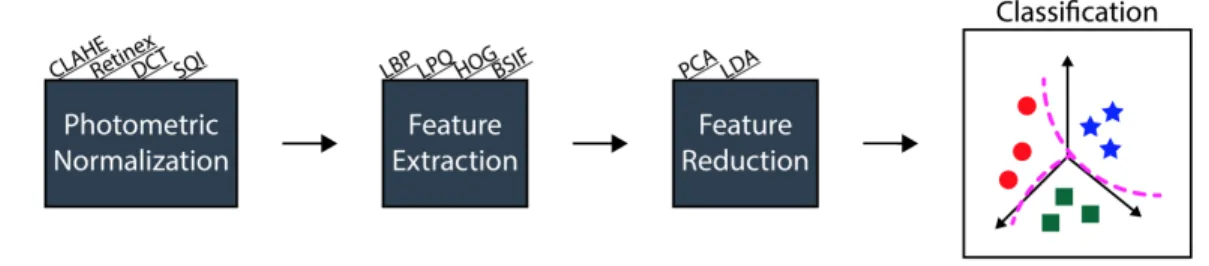
of this pipeline, the images are put through photometric normalization using one

of four methods: contrast limited adaptive histogram equalization (CLAHE), the multi-scale retinex algorithm, the discrete cosine transform (DCT)

algo-rithm, or the single scale self quotient (SQI) image algorithm. In the second stage of this pipeline, features are extracted using local binary patterns (LBP),

local phase quantization (LPQ), histograms of oriented gradients (HOG), and binarized statistical images (BSIF). Finally, these features are consolidated

us-ing Principal Component Analysis (PCA) or Latent Dirichlet Allocation (LDA),

1_{The following pipeline example was provided by Thomas Swearingen and Dr. Arun Ross of}

Michigan State University’s i-PRoBe Lab and has been incorporated into Deep Mining. We want to thank Thomas and Dr. Ross for their help in implementation and testing.

(32)

Figure 3-1: Illustration of the portion of the facial recognition pipeline to optimize.

and either a Random Forest Classifier or Support Vector Machine (SVM) is

ap-plied to the data.

2. Implement the chosen pipeline

Next, the data scientist must implement this pipeline by constructing its custom

steps, writing wrapper functions for feeding the intermediate transformations to subsequent pipeline steps, fitting classifiers, and outputting the eventual score.

This process involves either writing the code from scratch or copying code for the desired pipeline steps from other libraries. Both choices may involve significant

debugging in both constructing the steps and placing them inside a pipeline.

3. Import dataset

After this implementation, the data scientist must import this dataset in a

format suitable for the constructed pipeline.

4. Specify hyperparameters and ranges

Once the pipeline has been chosen, the data scientist must ensure that the

hy-perparameters for each of the step are exposed. The data scientist also chooses possible ranges for each of the hyperparameters, confining the search within

those bounds.

5. Tune hyperparameters

The data scientist can now tune the hyperparameters of the pipeline, using

(33)

example, because the pipeline has custom steps and includes more than con-ventional feature transformations (e.g., PCA, LDA) and classifiers, the data

scientist can use a system in the “black box function” paradigm, in which he provides a scoring function interface and tests inputs suggested by the

hyper-parameter optimizer.

6. Speed up pipeline evaluation for hyperparameter tuning

The hyperparameter optimizer requires scores for dozens of hyperparameter

sets in order to build a meta model and tune the whole pipeline. Because the pipeline is computationally intensive and the dataset is large, evaluation of each

of these sets can take hours. In order to find a solution in a reasonable time, the data scientist often implements a parallelization framework for simultaneous

hyperparameter set evaluation by launching multiple worker machines (say, on an Amazon cluster) and writing supporting software.

If the pipeline evaluation remains too slow, the data scientist implements sam-pling techniques to further speed up this process, getting approximate scores

for hyperparameter sets by using only parts of the dataset. He chooses these parts arbitrarily, taking random subsamples of the original data.

7. Output predictions for new data

Finally, the data scientist receives the highest-scoring hyperparameter set and

trains a model with those hyperparameters, altering his existing pipeline code if necessary. He then outputs his predictions on new data, either noting the

pipeline performance on this new data or using these newly formed predictions in production.

This process illustrates a number of the difficulties that data scientists will face even with the widespread availability of hyperparameter tuning systems. Lack of

automation and support in each of these steps makes for a labor-intensive and error-prone process. Constructing a pipeline is difficult without examples from domain

(34)

by many machine learning methods takes significant time. Many existing hyperpa-rameter optimization systems are entirely unsuited to this particular domain-specific

problem, and the black box function API provides no support for pipeline specifica-tion. Real-world problems require efficiently evaluating hyperparameter sets, and the

data scientist may spend significant time implementing a parallelization and sampling framework to speed up the model evaluation process. Even after he has found the

best hyperparameters in the space, using that information to train a model and make predictions requires additional software construction and debugging.

To solve this problem, we propose Deep Mining, a system for sequential hyperpa-rameter optimization that scales to complex pipelines and large datasets and provides

the necessary frameworks for solving the particular problems data scientists face. In this thesis, we also describe an alternative approach to accelerating hyperparameter

optimization using a subsampling algorithm called the Bag of Little Bootstraps.

3.1 Sampling-based Approach for Hyperparameter

Search

Much of hyperparameter optimization theory focuses on improving the models and

algorithms exploring the hyperparameter space. In this framework, the focus is on reducing the number of hyperparameter sets evaluated. However, the ultimate goal of

these automated model selection methods is to reduce the human and computational time it takes to optimize, and the number of model evaluations is only a proxy for

that metric. The contrarian approach we outline in this work is to reduce the time needed for the evaluation of a single hyperparameter set. We reduce this time using

two methods: 1) intelligent sampling, and 2) distributed computation. By focusing on reducing the time necessary for each model evaluation along with intelligently

choosing hyperparameter sets, Deep Mining significantly improves the time needed for hyperparameter optimization.

(35)

[31], which executes a grid search of hyperparameters in a distributed fashion. Work has also been done in deep neural networks to extrapolate the learning curve in

early epochs so as to stop model evaluations that are not promising [13]. Multi-task Bayesian optimization is also promising, as hyperparameter evaluations on smaller

datasets are used to predict performance on larger datasets [41]. The effects of random sampling on hyperparameter optimization have also been explored [20].

3.2 The Deep Mining System

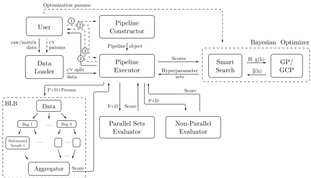
Deep Mining is an automated system that begins with raw or matrix-formatted data and ends with a tuned predictive model. Figure 3-2 illustrates the Deep Mining

system, detailing its major components and their interactions, which aim to provide the functionalities neglected by existing hyperparameter tuning systems.

The end-to-end system in Deep Mining provides these essential functionalities: solving the difficulties that come with non-standard pipeline specifications and

im-plementations, allowing importing of a variety of datasets, exposing hyperparameters, speeding up hyperparameter tuning, and aiding the use of pipelines in production.

In this project, we explore these functionalities along with higher-level goals.

This project spans various research areas: meta- machine learning (by pursuing novel meta modeling techniques using copulas), systems engineering (by

incorporat-ing data and distribution frameworks to enable parallel computation), human-data interaction (by designing an API that enables domain experts to share, compose and

tune novel/arbitrary pipelines), statistics (by incorporating sampling bootstrapped estimation), and ultimately artificial intelligence (by pursuing automation of steps

otherwise performed by data scientists).

State-of-the-art model of the hyperparameter space: To provide a competitive hyperparameter tuning system and to efficiently select points in the hyperparameter

space for evaluation, the model of the hyperparameter space and the resulting acqui-sition algorithm must improve upon existing methods. The Gaussian Copula Process

(36)

Data Loader Multinomial Sample 1 Aggregator User Data BLB Bayesian Optimizer Optimization params Pipeline object raw/matrix data CVparams CV split data Scores Score Score Score P+D P+D+Params P+D Hyperparameter sets H, g(h) g(h) Bag 1 ... Bag S Pipeline Constructor Pipeline

Executor SearchSmart GCPGP/

Parallel Sets

Evaluator Non-ParallelEvaluator ... ... ... 1 2 3 4

Figure 3-2: Illustration of the Deep Mining system’s functionality. The user specifies a pipeline using the provided framework, providing hyperparameter ranges and the necessary pipeline steps to the pipeline constructor and executor. The user also pro-vides the data in either raw or matrix format and cross-validation parameters to the data loader as well as optimization parameters to the Bayesian optimizer. Outside of the user’s view, Deep Mining constructs a scoring function using the provided pipeline and parameters, incorporating distribution and sampling to accelerate the evaluation process. Deep Mining also loads the data into a cross validation split for the pipeline executor, which chooses between different parallel and non-parallel evaluation meth-ods that return a score to the pipeline executor. The Bayesian optimizer interfaces with the pipeline executor, suggesting hyperparameter sets to evaluate given scores for previous sets. Within the Bayesian optimizer, the Smart Search algorithm pro-vides previous hyperparameters 𝐻 and associated scores 𝑔(ℎ) to the GP or GCP model, receiving an estimate ˆ𝑔(ℎ) of the scoring function in return. Finally, the pipeline executor returns the tuned pipeline and (optionally) tested hyperparameters and associated performances. In this figure, the labels are as follows: (1) corresponds to the hyperparameter ranges; (2) to the (custom) pipeline steps; (3) to the tested hyperparameters and associated performances; (4) to the pipeline with the best hy-perparameter set; and “P + D + Params” to the scikit-learn Pipeline object, data, and BLB hyperparameters.

(37)

system that allows for the flexible marginal distributions appropriate for models of the hyperparameter space. We describe this method in detail in Chapter 4.2.

Sampling algorithm to accelerate model evaluation: We use a model

selec-tion algorithm derived from Bag of Little Bootstraps, a sub sampling based approach that evaluates functions of data (over sub samples) with the same statistical

guaran-tees as the traditional bootstrap. The Bag of Little Bootstraps algorithm provides a significant asymptotic improvement to the evaluation of hyperparameter sets for a

variety of algorithms by taking advantage of weighted representations of data. We experiment with using this system to show that even with these asymptotic

improve-ments, the improvement in model performance from hyperparameter tuning remains comparable. We describe this method in detail in Chapter 6.

Distributed computation for parallel execution: Executing pipelines in a par-allel, distributed fashion significantly speeds up the evaluation process. By using

frameworks including Apache Spark, we can compute either the pipeline score on multiple bootstrap in parallel or compute scores for multiple different pipelines in

parallel. Deep Mining provides hyperparameter optimization at the scale demanded by modern applications. We describe our parallelization framework in detail in

Chap-ter 7.

Abstractions for arbitrary datasets and pipelines: Deep Mining offers an

al-ternative to the black box approaches used by existing hyperparameter systems by allowing composition of arbitrary pipelines and allowing ingestion of different data

types. Using the Pipeline interface from scikit-learn [35] and a custom API, users specify arbitrary pipelines operating either on matrices (as in other systems) or on

the raw data itself, seamlessly enabling the tuning of feature engineering methods that are unavailable in other auto-tuning systems. We describe how to compose arbitrary

pipelines using our api in Chapter 5.

As a consequence of this approach, we do not seek out performances on benchmark

datasets to show the superiority of our tuning algorithm or machine learning method suite. Instead, we enable pragmatic applications such as face recognition. By using a

(38)

feature extraction methods that do not operate on data in matrix format and provides utilities for using the tuned model in production.

Open-source software for collaborative data science: By providing abstractions for constructing and combining custom pipeline steps, Deep Mining incorporates the

input of various domain experts. Domain experts can contribute to the library by providing custom pipelines and software for data transformations. Systems

program-mers can contribute in tuning the distributed frameworks used, and statisticians can improve existing copula processes and subsampling methods.

(39)

Chapter 4 Gaussian Copula Processes

In this chapter, we will describe the Gaussian process (GP), which is often used to model the hyperparameter space, and introduce Gaussian Copula Processes (GCP)

as an improvement on traditional GP, detailing algorithms used by Deep Mining in hyperparameter search. The author acknowledges Kalyan Veeramachaneni and

Sébastien Dubois for their development of and help in describing the GCP method [14].

In this chapter, we use 𝑥 as the input vector, 𝑦 as the outcome that GP or GCP is trying to model, and 𝑓 as the unknown function that relates 𝑓 (𝑥) ← 𝑦. In the

context of hyperparameter tuning they are ℎ, 𝑦, and 𝑔 respectively.

4.1 Gaussian Processes

The Gaussian Process is a non-parametric method that allows for inference over the continuous space of functions. The chief insight it provides for tuning purposes is

that it allows for the construction of a Bayesian model of the hyperparameter space that updates with additional observations and is not confined to a specific functional

form. Much of the background in this section is based on work in [36], which can provide additional detail.

Definition 4.1.1. Gaussian Process (GP) A collection of random variables, any finite

(40)

A GP can be completely defined by its mean and covariance functions, which are functions of (multidimensional) locations in the input space. The mean function at a

location x in the space is:

𝑚(x) = E[𝑓 (x)] (4.1)

and the covariance function is:

𝑘(x, x′) = E[(𝑓 (x) − 𝑚(x))(𝑓 (x′) − 𝑚(x′))] (4.2)

The mean function is the average of the known function 𝑓 values and is typically taken to be zero, assuming centered data. A typical covariance function used is the

Squared Exponential (SE) covariance function:

𝑐𝑜𝑣(𝑓 (x), 𝑓 (x′)) = 𝑘(x, x′) = 𝑒𝑥𝑝(−1 2|x − x

′_|2

) (4.3)

The function in the hyperparameter search case is the model performance (e.g., accuracy) or loss, and the Gaussian process is used as a prior for that function over

the hyperparameter space. Predictions in this space are made using a posterior dis-tribution that has been conditioned on hyperparameter sets x1, ..., x𝑁 and their

as-sociated performances 𝑓 (x), ..., 𝑓 (x𝑁). The posterior distribution is used to evaluate

acquisition functions for a number of candidates in the space, and the value of these

acquisition functions is used to determine which hyperparameter set should be evalu-ated next, based on the data and the machine learning method to be tuned. I describe

those acquisition functions used in Deep Mining in Section 4.2.

The computational complexity of using a GP for hyperparameter optimization

be-comes clear upon examination of the expressions for the predictive mean and variance. The predictive mean is then

𝐾(𝑋*, 𝑋)[𝐾(𝑋, 𝑋) + 𝜎𝑛2𝐼] −1

𝑦 (4.4)

where 𝐾(𝑋, 𝑋) is the kernel matrix for all previous observations, 𝐾(𝑋*, 𝑋) is the

(41)

the observation noise (assuming 𝑦 = 𝑓 (x) + 𝜖), 𝐼 is the 𝑁 x 𝑁 identity matrix, and 𝑦 is the vector of previous observations.

The predictive variance is

𝐾(𝑋*, 𝑋*) − 𝐾(𝑋*, 𝑋)[𝐾(𝑋, 𝑋) + 𝜎𝑛2𝐼] −1

𝐾(𝑋, 𝑋*) (4.5)

The asymptotic complexity of this Gaussian process, then, is dominated by the inversion of the 𝑁 x 𝑁 kernel matrix. This results in an overall complexity of 𝑂(𝑁3_),

where 𝑁 is the number of (hyperparameter set, performance) observations. More detail on the Gaussian Copula Process and other aspects of this thesis can be found

in the related published paper [1].

4.2 Gaussian Copula Process (GCP)

The Gaussian Copula Process, introduced in [45], is a prior based on a GP that can

more precisely model the multivariate distribution of 𝑓 (x). A mapping Ψ : 𝒴 → 𝒵

transforms the output of 𝑓 into a new variable 𝑧. We define a new function 𝑔,

𝑔 : 𝒳 → 𝒵, and a combination of 𝑓 and Ψ given by 𝑔(𝑥) = Ψ(𝑓 (x)); and we model 𝑔 with a GP.

By doing this, we actually change the assumed Gaussian marginal distribution of each 𝑓 (𝑥) into a more complex one. This is because the Gaussian prior on 𝑔(𝑥) yields

the prior for 𝑓 (x) given by the following cumulative distribution function:

𝐹 (𝑦) = Φ(Ψ(𝑦)), (4.6)

where 𝐹 (𝑦) = P(𝑓 (x) ≤ 𝑦) and Φ is the standard univariate Gaussian cumulative distribution function.

So far in the literature [45, 38], a parametric mapping is learned so that 𝑔(𝑥) is

(42)

Ψ−1 by {𝑎𝑗, 𝑏𝑗, 𝑐𝑗} such that: Ψ−1(𝑧; {𝑎𝑗, 𝑏𝑗, 𝑐𝑗}𝐾𝑗=1) = 𝐾 ∑︁ 𝑗=1 𝑎𝑗𝑙𝑜𝑔(︀𝑒𝑏𝑗(𝑧+𝑐𝑗)+ 1)︀, (4.7)

with 𝑎𝑗, 𝑏𝑗 > 0. The authors are interested in predicting the values of a positive

function 𝑓 . In the general case, we can add another variable 𝑚:

Ψ−1(𝑧; {𝑎𝑗, 𝑏𝑗, 𝑐𝑗}𝐾𝑗=1, 𝑚) = 𝐾

∑︁

𝑗=1

𝑎𝑗𝑙𝑜𝑔(︀𝑒𝑏𝑗(𝑧+𝑐𝑗)+1)︀ −𝑚,

where 𝑚, 𝑎𝑗, 𝑏𝑗 > 0. For 𝐾 = 1 we then have :

Ψ(𝑦) = 𝑙𝑜𝑔(𝑒

𝑦+𝑚

𝑎 − 1)

𝑏 − 𝑐, 𝑚, 𝑎, 𝑏 > 0. (4.8)

However, this mapping is unstable in practice: we found that over many trials on the same dataset, different mappings were learned. Moreover, the induced univariate

distribution for 𝑓 (x) was almost Gaussian most of the time, and the parametric mapping did not offer great flexibility. We see in eq. (4.7) that for 𝐾 = 1, if 𝑏𝑧 >> 𝑏𝑐, 1, then Ψ−1(𝑧; 𝑎, 𝑏, 𝑐)∼ 𝑎𝑏𝑧, ie. the mapping is linear, and the GCP is actually a GP.

Given this observation, we introduce a novel approach where a marginal distribu-tion is learned from the observed data through kernel density estimadistribu-tion [37] of 𝐹 .

After this, the mapping Ψ is numerically computed from equation (4.6), so that the observations of the training data 𝑔(𝑥𝑡,𝑖) have a Gaussian distribution:

Ψ(𝑦) = Φ−1(𝐹𝑒𝑠𝑡(𝑦)). (4.9)

As the mapping function is learned in a non-parametric manner, we call this novel

(43)

Non-Parametric Latent GCP (nLGCP)

The prior mean of a Gaussian process is usually fixed as the empirical mean of the observations 𝑓 (𝑥𝑡,𝑖). In the context of hyperparameter optimization, however, one

can imagine that there should be some region where the hyperparameters would be rather good and others where they would be rather bad. For this reason, it may be

convenient to set a different mean for the prior, depending on the region in which the hyperparameter is. When it comes to GP, researchers assert that this alteration

would have little impact, as the covariance function is already meant to induce this smoothness. With GCP, however, we not only fix the mean function, but the mapping

function as well. Because the mapping function reflects the distribution of the data, with nGCP a latent model aims at learning several distributions of 𝑓 (x) over the input

space. In particular, this change may facilitate the location of promising regions to explore in a Bayesian optimization process.

We introduce a non-parametric Latent Gaussian Copula Process prior (nLGCP),

where the mapping function also depends on the input x. Intuitively, the goal is to include in the prior not only the distribution 𝒟 of 𝑓 (x) on the entire space 𝒳 but

the distributions 𝒟1, ..., 𝒟𝑘 of 𝑓 (x) on 𝑘 regions of 𝒳 . This way, we design a prior

that truly depends on 𝑥 (in the previous equations, 𝑥 was only an index to denote the random variable 𝑓 (x)).

To design the nLGCP prior, we look for a mapping function that depends on the

input 𝑥 and output 𝑓 (x). To construct this function, the training data {(𝑥𝑖, 𝑓 (𝑥𝑖))}

are clustered in 𝒳 × 𝒴 ⊂ R𝑚+1 _{using K-means. For each cluster 𝑘, a mapping Ψ} 𝑘 is

learned, as described in the previous section. Then, for each 𝑥 in 𝒳 , the final mapping Ψ is computed as Ψ(𝑥, 𝑦) =∑︁𝛼𝑘(𝑥).Ψ𝑘(𝑦), (4.10) where 𝛼𝑘(𝑥) = 𝑒𝑥𝑝(−𝑠∑︀ (𝑑_𝜎𝑘 𝑘) 2_{), 𝑑} 𝑘 = 𝑑𝑖𝑠𝑡𝒳(𝑥, 𝑐𝑘), 𝜎𝑘 = 𝑠𝑡𝑑𝒳(𝒞𝑘), 𝑠 is a smoothing

(44)

Predictions with nLGCP

Predictions with GP are straightforward given a posterior, but this calculation is no longer simple with nLGCP. A faster but approximate way to compute the predicted

value of 𝑓 (𝑥*) for a given 𝑥* is to calculate 𝑔*, the standard GP prediction of the

warped output Ψ(𝑓 (𝑥*)) given by the posterior: 𝑔(𝑥*) ∼ 𝒩 (𝜇*, 𝜎*), Noting from

the equation (4.6) that the predicted cumulative distribution function of 𝑓 (𝑥*) is

𝐹* = Φ(Ψ; 𝜇*, 𝜎*), we can evaluate the prediction as:

𝑓* =

∫︁ ∞

𝑢=−∞

𝑢.Ψ′(𝑢).𝜑(Ψ(𝑢); 𝜇*, 𝜎*).𝑑𝑢 (4.11)

where 𝜑𝜇*,𝜎*denotes the probability density function of a univariate Gaussian 𝒩 (𝜇*, 𝜎*).

The particular expression of Ψ in eq. (4.9) for the nGCP prior finally enables us

to express directly its derivative:

Ψ′_{𝑛𝐺𝐶𝑃}(𝑦) = 𝑑𝑒𝑠𝑡(𝑦)

𝜑(Ψ(𝑦)), (4.12)

where 𝜑 and 𝑑𝑒𝑠𝑡 are respectively the probability density function of the standard

univariate Gaussian and the one corresponding to 𝐹𝑒𝑠𝑡 defined in Section 4.2. We can

(45)

Chapter 5 Composing arbitrary pipelines

An overarching goal of this work is to enable the tuning of an entire pipeline, which

includes preprocessing, data transformations and feature extraction. This process presents several challenges:

∙ Too many possibilities: When considering data science pipelines, numerous possibilities exist for early-stage data transformations. Transformations can

be specific to domain or problem as well as specifically developed to mitigate issues in data collection. Because of this variety, developing a fixed set of

transformations a priori is impossible. These steps also accept a variety of inputs, such as data in non-matrix formats, that many existing tools cannot

incorporate.

∙ Unstructured process: Unlike software for machine learning algorithms, soft-ware for these transformations are written by domain experts, who do not in general construct the code for this part of the process in a structured and

uni-form way. This lack of structure and uniuni-formity inhibits code sharing and slows the development process.

A good pipeline specification must also be easy to use, in order to encourage adop-tion and pipeline experimentaadop-tion, and modular, allowing data scientists to combine

(46)

5.1 Abstractions for data transformation steps

Pipelines consist of series of data transformation steps ending with a modeling step in which a machine learning model is trained and evaluated. We call the steps that

transform the data Transformers and the step that trains and evaluates the model an Estimator1_{. To be able to develop generalized abstractions for programmatically}

defining transformers, we categorize them based on their input, output, and type of computation involved.

Type of computation: Transformers can be classified into two groups:

∙ Direct methods: These methods allow transformations on data to be com-puted using only the function and its hyperparameters without requiring any

learning of parameters from the data itself. An example of this type of method is patch extraction from a collection of images. For this category of methods,

the applied transformation can be defined simply:

𝑓 (𝑥𝑜𝑙𝑑) = 𝑥𝑛𝑒𝑤 (5.1)

where 𝑥 represents a single data point (a single image, a single text, or a feature

vector), and the function 𝑓 is applied to all data points in the entire dataset 𝑋.

∙ Fitted methods: Other transformers require parameters to be learned before transformations can be applied to the data. An example of this type of trans-formation is PCA, which must learn parameters from the structure of the data

before applying its transformations. Two sub-types of learning exist within this methods:

– Fitting using individual data points: In this category, transformer methods learn parameters from individual data points:

𝑝𝑎𝑟𝑎𝑚𝑠 = 𝐿(𝑥𝑜𝑙𝑑) (5.2)

(47)

then apply a transformation function using those parameters:

𝑓 (𝑥𝑜𝑙𝑑, 𝑝𝑎𝑟𝑎𝑚𝑠) = 𝑥𝑛𝑒𝑤 (5.3)

– Fitting using all data points: Transformer methods can also learn

parameters using the entire dataset and can be expressed as:

𝑝𝑎𝑟𝑎𝑚𝑠 = 𝐿(𝑋𝑜𝑙𝑑) (5.4)

then applying a function to the entire dataset using those global parameters

𝑓 (𝑋𝑜𝑙𝑑, 𝑝𝑎𝑟𝑎𝑚𝑠) = 𝑋𝑛𝑒𝑤 (5.5)

PCA and Bag-of-words are examples of transformers that learn the

pa-rameters for the transformation function using all the data points.

Data input and output: Transformers vary in terms of the input data format they

accept. Data domains broadly fall into four categories, which each require a uniform structure for designing transformers.

∙ Image data: For image datasets, regardless of the original data file type (e.g., jpeg, png), the raw image can be represented as a multidimensional array of numeric values corresponding to pixels. A flattened representation of the images

represents each image as a row in a matrix. The intermediate transformations for images therefore typically map between matrices of floating point or integer

values.

∙ Text data: For text datasets, the initial data can again be represented as a matrix, where each row corresponds to a different text document (data point).

The data types within the matrix eventually change from strings to numeric values. Transformations for text data, then, fall entirely within the categories

(48)

∙ Relational Data: Relational data undergoes the most stark transformation before eventual classification or regression. This type of data begins as a set of

tables, which are eventually consolidated into a feature matrix over the course of the pipeline before presenting it to the classifier or regressor. Transformers

for relational data have more complicated mappings than the typical matrix-to-matrix scheme, often going from “a set of tables” to a transformed “set of

tables” or consolidating “ a set of tables” into one. These transformations also often require meta data about data types of the variables in the tables and the

relational structure between the tables. Combinations of these data types can also have this characteristic, as the consolidation of varied data sources into an

eventual matrix format requires transformers with more complicated mappings. Once data is in matrix format, all transformer methods once again fall into the

categories for image and text data.

∙ Time series data: In time series data, each data point is a collection of ob-servation arrays along with an additional array corresponding to a time stamp, sequence number, or order number for the values in the other arrays.

Trans-formers can output another time series given a time series or consolidate them into a vector.

5.2 Abstractions for the pipeline

Once these Transformer and Estimator pipeline steps have been specified as Python functions, a unifying framework is necessary to ensure that (1) intermediate outputs

are correctly piped between steps (2) the pipeline can be used for training and pre-diction. Data scientists often construct a wrapper function that will take as input

all hyperparameters for the pipeline and data and contains the end-to-end training pipeline code. This function outputs all of the “fitted” parameters across all steps. A

separate wrapper function that takes as input the learned set of parameters and data is written to execute the pipeline given the learned parameters and produce

(49)

these functions for each problem it is an error-prone and time consuming process. A generalizable framework to solve this problem must allow users to:

∙ Easily compose the pipeline using only functions for each pipeline step without constructing extensive wrapper functions

∙ Effectively expose hyperparameters for all pipeline steps,

∙ Provide a simple command to train or “fit” the pipeline steps, saving fitted parameters and any meta data associated with the fitting process,

∙ Output a performance metric on a training dataset, and

∙ Provide a simple command to “predict” using the fitted pipeline.

5.2.1 Abstractions in scikit-learn

Scikit-learn, a popular machine learning software library, offers a powerful fit-transform

abstraction that greatly simplifies the process we describe above. It has the previously mentioned two types of object: transformers and estimators.

Transformer objects transform the data, and must have fit and transform meth-ods implemented, as the fit method allows them to learn parameters to be used for

transform. Given this object-oriented approach, a data scientist can

– Call transformer.fit_transform(X), which first “fits” using the data 𝑋 and then outputs the transformed version of the data, 𝑋𝑛𝑒𝑤.

– Call transformer.transform(X), which uses the fitted parameters from

trans-forming 𝑋 to output 𝑋𝑛𝑒𝑤.

Principal Component Analysis (PCA) is an example of a transformer that must fit itself before transforming the data. The fit method in PCA identifies the principal

vectors in the data, which are then used to transform the feature matrix. All trans-former methods in scikit-learn are written this way, enforcing uniformity across

(50)

Estimators, which make predictions using a fitted model, must implement fit and predict methods. Any machine learning classifier is an example of an estimator.

This fit-transform abstraction is also seen in various forms in other machine

learn-ing libraries, includlearn-ing Apache Spark’s MLlib and Keras [8].

With these abstractions and provided library of functions, scikit-learn allows the user to do the following:

∙ Create arbitrary pipelines: A user can chain together multiple transformers, provided the last step in each pipeline is an estimator method. Consider an example in which a user has a pipeline consisting of steps A, B, and C, where

A and B are scikit-learn transformers and C is a scikit-learn estimator. First, the pipeline object is constructed by specifying a list of the variables for

the pipeline steps. These variables denote objects on which the fit and transform methods can be called.

pipeline = Pipeline([A, B,C])

Next, the pipeline hyperparameters are mapped to individual steps:

pipeline.set_params = {A__a1: 𝑣𝑎1, B__b1: 𝑣𝑏1,

C__c1: 𝑣𝑐1}

where 𝑎1 is a hyperparameter for step A and 𝑣𝑎1 is the corresponding name

specified for the same in the overall hyperparameter dictionary. Deep Mining provides a wrapper to simplify this parameter setting, as detailed in section

5.4.1.

∙ Integrate training and validation: One of the advantages of setting up the pipeline object and mapping up the hyperparameters as shown above is that

now users can call the same “fit” and “predict” functions provided for individual steps to execute the entire pipeline. This functionality eliminates the need for

Deep Mining : scaling Bayesian auto-tuning of data science pipelines

Deep Mining: Scaling Bayesian Auto-tuning of Data

Science Pipelines

by

Alec W. Anderson

S.B., Massachusetts Institute of Technology (2017)

Submitted to the Department of Electrical Engineering and Computer

Science

in partial fulfillment of the requirements for the degree of

Master of Engineering in Electrical Engineering and Computer Science

at the

MASSACHUSETTS INSTITUTE OF TECHNOLOGY

September 2017

c

○ Massachusetts Institute of Technology 2017. All rights reserved.

Author . . . .

Department of Electrical Engineering and Computer Science

August 14, 2017

Certified by . . . .

Kalyan Veeramachaneni

Principal Research Scientist

Thesis Supervisor

Accepted by . . . .

Christopher J. Terman

Chairman, Masters of Engineering Thesis Committee

Deep Mining: Scaling Bayesian Auto-tuning of Data Science

Pipelines

by

Alec W. Anderson

Abstract

Acknowledgments

Contents

List of Figures

List of Tables

Chapter 1

Introduction

1.1

Automating what a data scientist does

1.2

Deep mining

1.3

Contributions

1.4

Previous Work

1.5

Outline

Chapter 2

Background and Related Work

2.1

Search Algorithms and Meta-modeling

2.1.1

Meta-modeling Approach

2.2

Choices of 𝑔

(h)

2.3

Current Hyperparameter Optimization Systems

Chapter 3

Deep Mining: Overview

3.1

Sampling-based Approach for Hyperparameter

Search

3.2

The Deep Mining System

Chapter 4

Gaussian Copula Processes

4.1

Gaussian Processes

4.2

Gaussian Copula Process (GCP)

Chapter 5

Composing arbitrary pipelines

5.1

Abstractions for data transformation steps

5.2

Abstractions for the pipeline

5.2.1

Abstractions in scikit-learn