HAL Id: hal-00296375
https://hal.archives-ouvertes.fr/hal-00296375
Submitted on 15 Nov 2007
HAL is a multi-disciplinary open access
archive for the deposit and dissemination of
sci-entific research documents, whether they are
pub-lished or not. The documents may come from
teaching and research institutions in France or
abroad, or from public or private research centers.
L’archive ouverte pluridisciplinaire HAL, est
destinée au dépôt et à la diffusion de documents
scientifiques de niveau recherche, publiés ou non,
émanant des établissements d’enseignement et de
recherche français ou étrangers, des laboratoires
publics ou privés.
weather prediction models
V. Venema, A. Schomburg, F. Ament, C. Simmer
To cite this version:
V. Venema, A. Schomburg, F. Ament, C. Simmer. Two adaptive radiative transfer schemes for
numerical weather prediction models. Atmospheric Chemistry and Physics, European Geosciences
Union, 2007, 7 (21), pp.5659-5674. �hal-00296375�
www.atmos-chem-phys.net/7/5659/2007/ © Author(s) 2007. This work is licensed under a Creative Commons License.
Atmospheric
Chemistry
and Physics
Two adaptive radiative transfer schemes for numerical weather
prediction models
V. Venema1, A. Schomburg1, F. Ament1,2, and C. Simmer1
1Meteorologisches Institut, Universit¨at Bonn, Auf dem H¨ugel 20, 53121 Bonn, Germany 2Meteo Schweiz, Numerical Models, Kraehbuehlstrasse 58, 8044 Zurich, Switzerland Received: 23 March 2007 – Published in Atmos. Chem. Phys. Discuss.: 30 May 2007 Revised: 18 October 2007 – Accepted: 30 October 2007 – Published: 15 November 2007
Abstract. Radiative transfer calculations in atmospheric models are computationally expensive, even if based on simplifications such as the δ-two-stream approximation. In most weather prediction models these parameterisation schemes are therefore called infrequently, accepting addi-tional model error due to the persistence assumption between calls. This paper presents two so-called adaptive param-eterisation schemes for radiative transfer in a limited area model: A perturbation scheme that exploits temporal correla-tions and a local-search scheme that mainly takes advantage of spatial correlations. Utilising these correlations and with similar computational resources, the schemes are able to pre-dict the surface net radiative fluxes more accurately than a scheme based on the persistence assumption. An important property of these adaptive schemes is that their accuracy does not decrease much in case of strong reductions in the num-ber of calls to the δ-two-stream scheme. It is hypothesised that the core idea can also be employed in parameterisation schemes for other processes and in other dynamical models.
1 Introduction
Parameterisations of subscale processes are indispensable for dynamical numerical weather prediction (NWP) and climate models. The atmosphere and the land surface are complex systems, which display variability over a large range of scales (Davis et al., 1999; Gagnon et al., 2006). Consequently, atmospheric models are only able to resolve a part of this range and NWP models will always need parameterisations for subscale processes. On the positive side, atmospheric variables are correlated temporally and spatially. These cor-relations will be exploited in the present paper to improve the efficiency of parameterisation schemes.
Correspondence to: V. Venema ([email protected])
The main goal of adaptive parameterisation schemes is to be able to apply parameterisations that are as physical as (computationally) possible. This will benefit, e.g. the trust-worthiness of climate change projections. In practice, there is a conflict between the required computational efficiency of the parameterization on the one hand and accuracy and its physical realism on the other hand. To mitigate this conflict, we developed the concept of an adaptive parameterisation scheme. In such a scheme a conventional parameterisation is split into two parts: an intrinsic and an extrinsic parame-terisation. The intrinsic parameterisation aims at reproduc-ing the subgrid-scale physical processes accurately. Conse-quently, it is computationally expensive and therefore called as infrequently as possible.
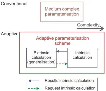
The division of labour is illustrated in Fig. 1, where the blue arrow running from the right to the left symbolises that the generalisation algorithm relies on information from the intrinsic calculation. The other direction can be important as well: the green dashed arrow running from the left to right denotes the possibility that the generalisation algorithm re-quests an additional intrinsic calculation to improve the ac-curacy.
The computationally efficient extrinsic parameterisation calculates the parameterised tendencies for all model boxes with a high temporal update frequency. The extrinsic param-eterisation can be a purely statistical algorithm or an efficient physical parameterisation. The key idea is that the extrsic parameterisation adapts itself to the tendencies of the in-trinsic calculations, which are close by in terms of space or time, and spreads these results to the full model field. This is why, with a focus on its computational features, we also call the extrinsic calculation, the generalisation. In this way, the scheme exploits the spatial and temporal correlations in the model fields to improve its efficiency. With the increase in the number of grid boxes, the spatial correlations between adjacent grid boxes will become stronger, favouring a transi-tion from traditransi-tional to adaptive parameterisatransi-tion schemes.
Intrinsic calculation Extrinsic
calculation (generalisation)
Request intrinsic calculation Results intrinsic calculation
Fig. 1. A schematic view of the concept of an adaptive
parameteri-sation scheme. The intrinsic parameteriparameteri-sation resolves the subgrid-scale processes. It is called as infrequently as possible to save com-putational resources. The extrinsic parameterisation utilises the out-put of the intrinsic calculation (blue arrow) and calculates tenden-cies for all grid boxes and time steps. The extrinsic parameterisation can also be employed to predict where or when an additional intrin-sic parameterisation will improve the accuracy of the scheme most (green arrow).
In the World Climate Research Programme (WCRP) it is argued that we understand small-scale processes reason-ably well, but that this knowledge still has not sufficiently led to better parameterisations in general circulation models (WCRP, 2004; Randall et al., 2003b). This is called the im-plementation bottleneck and is probably because the devel-opment of parameterisation schemes is a difficult and time-consuming art. We hope that adaptive schemes will make parameterisation development easier, as the amount of sim-plification from a detailed small-scale model to an intrinsic calculation will be less than the reduction to a conventional parameterisation.
As the radiation parameterisation needs a considerable amount of computational resources, weather services have aimed at reducing its cost. The dominant method in the time domain is the reduction of the frequency with which the scheme is called. A typical radiation time step is one hour (e.g. the COSMO-EU (the model of the COnsortium for Small-scale MOdeling in the configuration for EUrope; Steppler et al., 2003), the Global-Modell (GME; Majew-ski et al., 2002), the community atmospheric model (CAM; Collins et al., 2004) and the global spectral model of the ECMWF, European centre for medium-range weather fore-casts). Some models, however, have radiative time steps of 15 min, which is the standard time step of Meso-NH (Mesoscale non-hydrostatic model; Meteo France, 2002),
and of COSMO-DE, the COSMO model version for short-range forecasts. Meso-NH has the option to specify a smaller time step for cloudy columns. HIRLAM (High-resolution lo-cal area model; Und´en et al., 2002) used to employ a more approximate radiation scheme distinguishing only two spec-tral bands, in order to be able to call the scheme at each time step (Sass et al., 1994); today HIRLAM utilises ECMWF physics.
Between radiation time steps, longwave radiative fluxes are typically held constant; shortwave fluxes are either held constant (e.g. COSMO) or scaled to account for the changing solar incidence angle (e.g. ECMWF and GME). To avoid bi-ases due to the 1h-persistence assumption, the radiative trans-fer scheme of the COSMO model works with the solar zenith angle (SZA) of half an hour later, i.e. half its radiation time step.
Another approach to reduce the costs of the radiative trans-fer parameterisation is the employment of artificial neural networks (ANN). This way has been successfully imple-mented for the long wave radiative transfer scheme of the ECMWF and CAM (Chevallier et al., 1998; Chevallier et al., 2000; Krasnopolski et al., 2005). A more accurate alter-native to ANNs is the use of look-up-tables (Matsiu et al., 2004; Pielke et al., 2005). This method can also handle short wave radiative transfer, but requires a large look-up-table that needs to be stored on a hard disk.
Due to advection and cloud development within the ation time step, considerable errors may occur in the radi-ation fields. The persistence assumption can lead to physi-cal inconsistencies and removes the possibility of feedbacks on smaller temporal scales. Depending on the compromise that was made between call frequency and spatial resolution of the model, these schemes are either computationally ex-pensive or will suffer from errors due to the persistence as-sumption. Geleyn et al. (2005) are working on a scheme that is similar to our adaptive perturbation scheme (see Sect. 2) with the aim of achieving a high temporal frequency at ac-ceptable costs. This scheme builds on the net exchange rate method (Green, 1967) and computes the contribution of the gases with a lower update frequency than the perturbations due to clouds.
In space domain, a number of statistical interpolation methods are applied. Meso-NH has the option to perform one calculation for all cloud-free columns. Furthermore, there is an option to call the radiative transfer scheme only for some columns and to utilise bilinear interpolation for the non-selected ones (Meteo France, 2002). Until September 2004, the ECMWF called the radiative transfer scheme ev-ery fourth column and interpolated its values using a cubic interpolation scheme (Morcrette, 2000).
Nowadays, the ECMWF radiation scheme is operated at a lower spatial resolution than the resolution for the dynamics. Afterwards, the radiation tendencies are interpolated to the high-resolution columns. For the COSMO-DE, it is planned to calculate the radiation on a coarser grid in a similar manner
as the current ECMWF scheme. The model fields are av-eraged over 2×2 columns before calling the δ-two-stream scheme. Afterwards, in the distribution to the fine grid, the high-resolution albedo and ground temperature are taken into account (Baldauf et al., 2006; T. Reinhardt, personal commu-nication, 2006).
Except for the COSMO-DE, these interpolation schemes are purely statistical and do not take into account physical relationships between clouds, surface and radiation. They may thus lead to significant physical inconsistencies in the models. Furthermore, near cloud edges, the gradients in the radiation field will be smoothed away.
In this paper, we will present two adaptive parameter-isation schemes for the radiative transfer calculation of the numerical weather prediction model COSMO. The two schemes differ mainly in their generalisation methods. The generalisation in Sect. 2 exploits temporal correlations using a perturbation approach. In Sect. 3, the generalisation em-ploys a simple local-search algorithm, which primarily takes advantage of spatial correlations.
The COSMO model and its radiative transfer scheme are introduced in Sect. 4. The current radiative transfer algo-rithm will be utilised as the intrinsic calculation of both adap-tive schemes. This allows us to concentrate on the overall concept and on the development of the generalisations. With a case study, we will illustrate the concepts and show the con-siderable error reduction and the increase in efficiency these adaptive radiative transfer schemes can achieve. The setup of this case study is described in Sect. 4.3, together with a de-scription of a scheme based on the persistence assumption, which is introduced for comparison. The results of the two adaptive schemes are compared to the result of the persis-tence scheme in Sect. 5. The paper finishes with discussions, a summary and an outlook.
2 Temporal perturbation scheme
In this section and the next, the general idea of an adaptive parameterisation scheme will be illustrated by two adaptive schemes for radiative transfer in the COSMO model. The perturbation scheme in this section exploits temporal corre-lations in the atmospheric fields. This adaptive scheme com-bines a selection mechanism (green dashed arrow in Fig. 1) and a so-called perturbation algorithm (blue arrow).
The intention of the selection mechanism is to recalculate the radiation at those grid points and times where it is most needed. For the decision, whether to call the δ-two-stream scheme or not, a simple radiation scheme acts as a predic-tor for the changes in the radiative net fluxes at the surface (1Fjsimple(t )). The change predictor for a column j is the flux difference calculated by the simple scheme as the flux at
the current time step (Fjsimple(t )) minus the flux at the time step of the last exact update (Fjsimple(texact)):
1Fjsimple(t ) = Fjsimple(t ) − Fjsimple(texact). (1) This change estimator is calculated at high temporal resolu-tion (1t=5 min) for every column. For the twelfth part of the columns with the largest changes, the δ-two-stream algo-rithm is called. Consequently, summed up over one computa-tional hour, the same number of calls to the δ-two-stream al-gorithm is made as in the persistence scheme (see Sect. 4.3). Expecting that the generalisation is computationally inexpen-sive compared to the intrinsic calculation, the total computa-tional cost should not increase much.
If the δ-two-stream algorithm is not called, the perturba-tion algorithm calculates a correcperturba-tion increment based on the simple radiation scheme, which is added to the radiation fluxes of the last time step:
Fj(t + 1t ) = Fj(t ) + δF
simple
j
δFjsimple =Fjsimple(t + 1t ) − Fjsimple(t ). (2) The simple radiation scheme is realised by a multivariate re-gression, which has been trained and validated with three month of data (July to September 2004) from the 12:00 UTC operational analysis. For training every second column was utilised and for the validation the other half of the data.
The predictands in this regression are the solar transmis-sivity c and the infrared downwelling radiation flux at the surface L↓. The solar transmissivity is converted to the so-lar surface net flux taking into account the soso-lar zenith angle and the albedo of the ground. Four different regressions have been developed, each with its own set of predictors, namely for the shortwave and longwave region and for cloudy and cloud-free situations, respectively. Grid-scale and subgrid-scale clouds are in the same category.
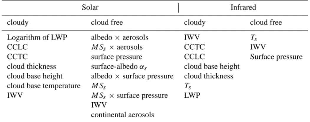
A list with the predictors in their order of importance is presented in Table 1. The root mean square errors (RMSE) for each of the four categories separately are presented in Table 2. The lowest number of predictors is necessary for describing cloud-free conditions in the longwave part of the spectrum. With the surface temperature, integrated water vapour (IWV) and surface pressure, the longwave radia-tion fluxes at the surface can be calculated with a RMSE of 7 W/m2, which is a relative error of 2%. A similarly small relative error is achieved for cloudy conditions in the longwave and for the cloud-free conditions in the shortwave regime, but additional variables are needed as predictors in these cases. Predictors of higher order are needed to account for multiple scattering between surface and atmosphere in the solar regime. The most difficult case to emulate with this simple scheme is cloudy grid boxes in the shortwave spec-trum. Predictors are several cloud properties and the IWV (see Table 1); the achieved RMSE is 68 W/m2, which corre-sponds to a relative error of 13%. Best results are achieved
Table 1. The predictors of the regression algorithm, ordered by their importance.
Solar Infrared
cloudy cloud free cloudy cloud free
Logarithm of LWP albedo × aerosols IWV Ts
CCLC MSs×aerosols CCTC IWV
CCTC surface pressure CCLC Surface pressure
cloud thickness surface-albedo αs cloud base height
cloud base height albedo × surface pressure cloud thickness
cloud base temperature MSs Ts
IWV MSs×surface pressure LWP
IWV
continental aerosols Aerosols: Total aerosol optical depth
CCLC: Cloud cover of low clouds CCTC: Total cloud cover IWV: Integrated water vapour LWP: Liquid water path
MSs: Term for multiple scattering at surface: αs/(1−αs) Ts: Surface temperature
taking the logarithm of the liquid water path (LWP) as pre-dictor. However, since subgrid-scale clouds do not have an explicit cloud water content in the COSMO, their LWP needs to be set to a small value (0.9 g m−2). These errors are con-siderable; another disadvantage of stand-alone regression al-gorithms is that they can produce large biases for a specific day.
3 Spatial local-search scheme
The second scheme relies on the spatial correlations in the field. To obtain the radiative tendencies for a certain col-umn, the generalisation searches in a small region around this point for a previous intrinsic calculation on a similar cloud column. The similarity between two columns is estimated mainly based on its cloud cover and liquid water path. In this way, this generalisation accounts well for advection of the cloud field.
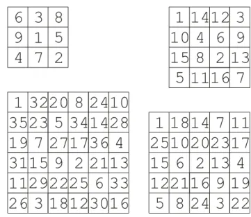
The details of the implemented algorithm are as follows. At the beginning of the model run, initial values are obtained by performing δ-two-stream calculations for the entire field. These values are stored in memory, together with their LWP, albedo and cloud cover fields, and time of calculation. Then, every five minutes, one additional intrinsic calculation is per-formed in small subregions of 4×4 columns. The selection of this column follows a regular pattern; see Fig. 2. These pat-terns were designed to have a large distance between consec-utive calculations and to be homogeneously spread over the subregion. With the standard 4×4 pattern, all columns are calculated once every 80 min, i.e. somewhat less often than the 60 min utilised in the persistence scheme (see Sect. 4.3).
Hence, about the same number of function calls are made, the main difference is that the adaptive scheme spreads these calls over the hour.
In the columns where no δ-two-stream calculations are performed for a certain 5-min time step, the generalisation algorithm determines the new radiative tendencies. To this end, the generalisation searches for similar nearby columns where previous intrinsic calculations were performed using the equation:
δ = w1|1CCL| + w2|1CCT| + w3|1LWP|
+w4|1αs| +w5|1t |, (3)
where δ is the similarity index to be minimised, wi are
weights, 1CCL is the difference for the cloud cover of low clouds between the current column and the stored columns on which intrinsic calculations were performed. 1CCT, 1LWP and 1αs are the same differences for the total cloud
cover, the liquid water path (LWP) and the surface albedo, re-spectively. Finally, 1t is the difference in time, i.e. how long ago the intrinsic calculation was performed. Low clouds are defined as the clouds in the levels below 800 hPa in the stan-dard pressure profile. The infrared surface net flux of the most similar nearby column is copied; the solar net flux is corrected for the change in surface albedo and solar zenith angle, in other words the transmittance of the most similar known column is taken.
This search is performed in a square region around the current column. The size of this region and the weights of Eq. (3) have been optimised based on the full δ-two-stream dataset; see Sect. 5.4 for details. This optimisation led to a search region of 7×7 pixels and the weights were adjusted
Table 2. Root mean square errors and relative errors of the
regres-sion scheme for the shortwave and longwave downwelling radiative fluxes at the surface for cloudy and cloud free conditions, respec-tively.
RMSE Error relative to Error relative to (W/m2) mean (%) standard deviation (%)
Solar Cloud free 18 2 16 Cloudy 68 13 31 Infrared Cloud free 7 2 22 Cloudy 10 2 29
such that the LWP is most important, followed by the cloud cover of low clouds, the albedo, the time difference and the total cloud cover; the importance of a parameter was esti-mated from the decrease in accuracy by omitting this param-eter. Section 5.1 will describe the results for the standard algorithm in relation to the other schemes. Section 5.4 will demonstrate that the results are insensitive to the optimisa-tion method and tuning constants. Furthermore, this secoptimisa-tion will investigate the scheme in more detail.
4 The modelling environment 4.1 The COSMO model
For this study, we utilised the output of the non-hydrostatic limited area model COSMO of the COnsortium for Small-scale MOdeling, formerly known as Lokal-Modell (LM) (Sch¨attler et al., 2005). The prognostic variables are the wind vector, pressure perturbation, air temperature, specific humidity of water vapour, cloud liquid water and ice, and precipitation in the form of rain, snow and graupel.
The COSMO model employs a spherical coordinate sys-tem with geographical longitudinal and latitudinal coordi-nates and a rotated pole. The vertical coordinate is a hy-brid vertical coordinate which is parallel to the surface in the lower levels and horizontal in the upper part. For the numer-ical time integration, we utilised the default scheme of the COSMO model, i.e. a three time-level Leapfrog scheme of second order.
Subgrid-scale clouds are parameterised by means of an empirical function depending on relative humidity, height, and convective activity. Moist convection is parameterised by the mass flux scheme of Tiedtke (1989) with a closure based on moisture convergence.
4.2 The radiative transfer scheme
The spectral radiation scheme of the COSMO model, which was developed by Ritter and Geleyn (1992), takes into ac-count emission, scattering and absorption by clouds, gases,
Fig. 2. The patterns of the calls to the intrinsic parameterisation by
the spatial scheme for the regions with size: 3×3, 4×4 (standard), 5×5 and 6×6.
aerosols and the land surface. It is based on the δ-two-stream approximation of the radiative transfer equation. In this ap-proach, the radiative transfer equation is solved in one di-mension, considering only two streams: the upward and the downward fluxes. The spectrum is divided into three regions in the solar regime and five in the thermal regime.
Each vertical layer is characterised by two sets of optical properties, one for the cloud-free part and one for the cloud covered part of the layer. The vertical cloud profile is mod-elled using the maximum-random overlap assumption, i.e. clouds in adjacent layers overlap fully, while the clouds in layers that are separated by a cloud-free layer are distributed randomly in the horizontal. The effective radius of the cloud droplets is parameterised as a function of the cloud water content.
The scheme considers effects of scattering and absorption by aerosols in all spectral intervals. The optical properties of five aerosol types are differentiated, namely continental, maritime, urban, volcanic and background stratospheric. The aerosols and gases (besides water vapour and ozone) are de-fined by a climatological map and do not change in time; ozone has a climatological annual cycle.
Operationally, the radiative transfer scheme is called once every hour and its surface net radiative fluxes and atmo-spheric heating rates are fixed until the next call. An impor-tant source of error is that the cloud field advects and de-velops during this hour (see Sect. 5.1 and Figs. 3 and 4). To avoid biases due to the 1h-persistence assumption, the scheme works with the solar zenith angle (SZA) of half an hour later.
(a) (b) (c) (d) (e) (f) 0 100 200 300 400 500 600 -4 -3 -2 -1 0 0.1 0.2 0.3 0.4 0.5 0.6 0 100 200 300 400 500 600 0 100 200 300 400 500 600 0 100 200 300 400 500 600 (g) RMS: 77 W m-2 Bias: 5 W m-2 -500 0 500 (h) RMS: 43 W m-2 Bias: 6 W m-2 -500 0 500 (i) RMS: 31 W m-2 Bias: 2 W m-2 -500 0 500
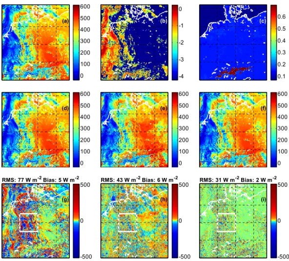
Fig. 3. An illustration of the errors in the solar net radiative flux (all in W m−2) in the COSMO model at the surface for 12:30 UTC. For
orientation, the boundaries between water and land are indicated with a white line. In the north-west is the North Sea and The Netherlands, in the north-east the Baltic Sea and in the south large lakes around the Alps are visible. The δ-two-stream calculation of the solar net flux is the reference field (a). Important related quantities are the liquid water path shown as log10(LWP/kg m−2) (b) and the surface albedo (c);
two cloud properties are depicted in Fig. 4. The second row shows the solar net flux fields calculated with the three standard methods: (d) the 1-h persistence scheme, (e) the adaptive perturbation scheme, (f) the adaptive search scheme. The corresponding errors are shown in the same order in the third row. The white box indicates the smaller region displayed in Fig. 6.
4.3 Case study
The proof of concept of the adaptive schemes will be based on a case study where the COSMO model was set up to call the radiative transfer calculation every 2.5 min, with output every 5 min. This reference run is treated as the truth, and will be employed to calculate the error made by the persis-tence scheme and the two adaptive schemes. 19 Septem-ber 2001 was chosen as it is a difficult day for the radiation scheme with much convection and thus large temporal and spatial variability in the cloud and radiance fields; see Figs. 3 and 4.
This case was computed with the COSMO model (ver-sion 3.16) at the resolution and modelling domain of the COSMO-DE. The horizontal resolution was 2.8 km (421×461 columns) and the grid has 50 vertical layers. The
domain is aligned in the north-south direction and centred on Germany. To remove boundary effects, only the middle 372×420 columns are displayed and analysed.
The prognostic precipitation scheme and the shallow con-vection parameterisation were utilised; deep concon-vection is assumed to be resolved by the model. Grid-scale clouds and precipitation are taken into account by a Kessler-type bulk parameterisation (Kessler, 1969) considering cloud wa-ter, rain, cloud ice, snow, and graupel (Reinhardt and Seifert, 2006).
We test the adaptive parameterisation methods offline, i.e. without feedbacks on the model integration: Based on the 5-min model output and radiative fields, we diagnose solar and infrared net fluxes at the surface from the two schemes and quantify the accuracy relative to the results of the refer-ence run. The schemes are tested by analysing the differrefer-ence
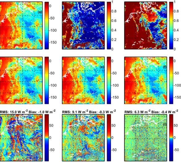
(a) (b) (c) (d) (e) (f) -150 -100 -50 0 0 0.2 0.4 0.6 0.8 1 0 0.2 0.4 0.6 0.8 1 -150 -100 -50 0 -150 -100 -50 0 -150 -100 -50 0 (g) RMS: 15.0 W m-2 Bias: -1.0 W m-2 -50 0 50 (h) RMS: 9.1 W m-2 Bias: -0.3 W m-2 -50 0 50 (i) RMS: 6.3 W m-2 Bias: -0.4 W m-2 -50 0 50
Fig. 4. An illustration of the errors in the infrared net radiative flux (cooling) rates (all in W m−2) in the COSMO model at the surface for
12:30 UTC. The δ-two-stream calculation is the reference field (a). Important related quantities are the cloud cover of low clouds (b) and the total cloud cover (c); two other radiatively important properties are depicted in Fig. 3. The second row shows the infrared net flux fields calculated with the three standard methods: (d) the 1-h persistence scheme, (e) the adaptive perturbation scheme, (f) the adaptive search scheme. The corresponding errors are shown in the same order in the third row.
between their predictions and the “truth” from δ-two-stream calculations on the entire domain.
For comparison, also a persistence scheme is tested where all intrinsic calculations are computed at the same time step and persistence is assumed between the time steps. Except where indicated otherwise, the radiation time step of this scheme is one hour. The persistence scheme computes the surface net radiative fluxes based on the model state at every full hour, but with the solar zenith angle of 30 min later to minimise bias errors. Consequently, we have chosen to let all schemes compute the surface net fluxes for 12:30 UTC.
5 Results
In this section, the adaptive schemes are put to the test by analysing the difference between their predictions and the “true” net fluxes at the surface. In the first subsection, the
statistical properties of the difference fields for the standard schemes are examined in detail. In Sect. 5.2 the relation be-tween the number of calls to the intrinsic parameterisation and the accuracy of the schemes is looked at. In the last two sections, the influence of variations of the two standard adap-tive schemes is investigated.
5.1 Error fields 5.1.1 Error magnitude
The central outcome is displayed in Fig. 3 (4) for the so-lar (infrared) surface net flux. Root mean square (RMS) errors and biases are presented in Table 3. The RMS error for the solar net flux of the persistence scheme is 77 W m−2, compared to 43 W m2 for the standard tempo-ral perturbation scheme and 31 W m−2for the standard spa-tial local-search scheme. This is 53%, 30%, and 21% of
Table 3. The RMS errors and biases in W m−2for the solar and the infrared net radiative flux for 12:30 UTC of various parameterisa-tion schemes.
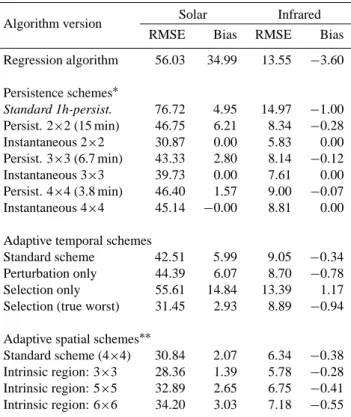
Algorithm version Solar Infrared
RMSE Bias RMSE Bias
Regression algorithm 56.03 34.99 13.55 −3.60 Persistence schemes∗ Standard 1h-persist. 76.72 4.95 14.97 −1.00 Persist. 2×2 (15 min) 46.75 6.21 8.34 −0.28 Instantaneous 2×2 30.87 0.00 5.83 0.00 Persist. 3×3 (6.7 min) 43.33 2.80 8.14 −0.12 Instantaneous 3×3 39.73 0.00 7.61 0.00 Persist. 4×4 (3.8 min) 46.40 1.57 9.00 −0.07 Instantaneous 4×4 45.14 −0.00 8.81 0.00 Adaptive temporal schemes
Standard scheme 42.51 5.99 9.05 −0.34 Perturbation only 44.39 6.07 8.70 −0.78
Selection only 55.61 14.84 13.39 1.17
Selection (true worst) 31.45 2.93 8.89 −0.94 Adaptive spatial schemes∗∗
Standard scheme (4×4) 30.84 2.07 6.34 −0.38 Intrinsic region: 3×3 28.36 1.39 5.78 −0.28 Intrinsic region: 5×5 32.89 2.65 6.75 −0.41 Intrinsic region: 6×6 34.20 3.03 7.18 −0.55
∗The persistence schemes at coarse resolution have two types of
error. The instantaneous error is the difference of the coarse and the high-resolution field at 12:30 UTC. An additional error is due to the persistence assumption; the applied radiation time step is given in brackets.
∗∗The intrinsic region is the subregion in which every 5 min one
intrinsic calculation is performed; the standard scheme has an in-trinsic region of 4×4 columns; see Fig. 2.
the standard deviation of the solar net flux field, respec-tively. The respective relative values for the infrared sur-face net flux are 40%, 24% and 16%. The bias for the solar net flux is slightly higher for the adaptive tempo-ral scheme (6.0 W m−2) than for the persistence method (5.0 W m−2), but the spatial scheme has the smallest bias of only 2.1 W m−2. In the infrared, the temporal scheme has the smallest error (−0.34 W m−2) compared to 0.38 W m−2 for the spatial scheme and −1.0 W m−2 for the persistence assumption.
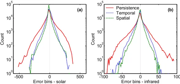
The error histograms in Figure 5 show that both adaptive schemes are similarly successful in eliminating the large er-rors (more than 200 W m−2for the solar flux or more than 40 W m−2in the infrared region). Especially the maximum errors are reduced considerably. The additional accuracy of the adaptive spatial scheme is due to a stronger reduction of the medium and small errors.
5.1.2 Correlation length error fields
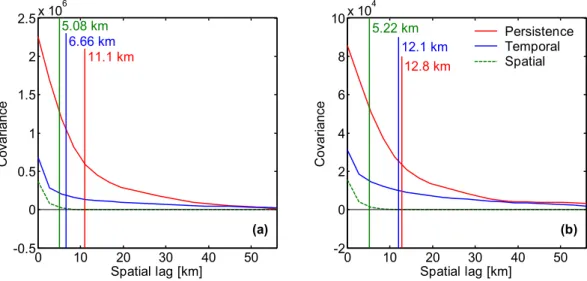
Not only the absolute errors are important, spatial and tem-poral correlations of the error fields determine their influence on model dynamics as well; see discussion. In Fig. 6, parts of the error fields are shown for a small subregion where a large amount of dynamical development can be found. The error field of the persistence scheme shows banded structures at cloud edges due to the phase error in the cloud field. This leads to a relatively long error correlation length (for the large domain) of 11 km in the solar regime and 13 km in the in-frared; see Fig. 7. The error correlation length of the tempo-ral scheme is somewhat less, especially for the solar surface net flux, namely 6.7 km and 12 km, respectively. The spa-tial scheme has the smallest error correlation length of all schemes, with an error correlation length of about 5 km for both the solar and the infrared regime.
5.1.3 Temporal and spatial resolution
The phase error in the cloud field is a consequence of the imbalance between the spatial and the temporal resolution of the persistence scheme. To reduce this imbalance, i.e. to find an optimal combination of the spatial and temporal resolu-tion, the radiative transfer calculation can be performed on a coarser grid, e.g. by computing on 2×2 columns simulta-neously as in the ECMWF model and in the COSMO-DE model. Keeping the computational costs the same, a 2×2 scheme can be called every 15 min. To model the error made by a perfect scheme of this type, we averaged the transmit-tance and the infrared net flux fields to a coarser grid. The RMS difference at 12:30 UTC between the high-resolution solar net flux and its coarse-grained counterpart is 31 W m−2 (see the row labelled “instantaneous 2×2” in Table 3). How-ever, a persistence error due to an average delay of 7.5 min has to be added. To this end, we averaged the errors of the coarse-grained fields 5 and 10 min before 12:30 UTC. The difference then increases to 47 W m−2; see the row labelled “Persist. 2×2” in Table 3. The best results were achieved in this idealised case with a coarse-grained parameterisation that averages the atmosphere over 3×3 columns and a per-sistence error due to a delay of 3.3 min. Coarse graining the model over 4×4 columns reduces the persistence error fur-ther, but increases the total error. Also coarse-grained pa-rameterisations can be converted to adaptive schemes. This calculation can only illustrate the problem of the phase error. To confirm that 3×3 columns is the optimal spatial resolu-tion, a more accurate calculation should be performed with a coarse-grained parameterisation in which the input fields are averaged and the coarse tendencies are disaggregated after-wards.
-500 0 500 100 101 102 103 104 105
Error bins - solar
(a) -100 -50 0 50 100 100 101 102 103 104 105
Error bins - infrared (b) Persistence
Temporal Spatial
Fig. 5. The histograms of the error in the solar (left) and infrared (right) regime for the three standard schemes: the 1h-persistence scheme
(red line), the adaptive temporal perturbation scheme (blue line) and the adaptive spatial local-search scheme (green dashed line). The bin widths of the error in the solar radiation are 20 W m−2and for infrared 2 W m−2.
(b) RMS: 117 W m-2 Bias: 12 W m-2 -500 0 500 (d) RMS: 41 W m-2 Bias: 2 W m-2 -500 0 500 (a) 0 100 200 300 400 500 600 (c) RMS: 49 W m-2 Bias: 6 W m-2 -500 0 500
Fig. 6. A zoom of the solar net flux at the surface (a) and its errors for the three different standard methods: (b) 1-h persistence scheme, (c)
5.1.4 Origins for the errors
The error of the adaptive temporal scheme correlates with the error of the persistence scheme (in the solar regime the correlation coefficient r=0.33; infrared: r=0.25). Even if the correlations are not high, this indicates that, as expected, dynamical situations where the persistence assumption leads to errors are also more difficult for the perturbation scheme. The error of the spatial scheme also correlates (solar: r=0.19; infrared: r=0.12) with the error of the persistence scheme, but the correlations are small.
In the Alps, the RMS errors of both adaptive schemes are about equal. The Alps represent a difficult region to the spa-tial scheme due to the minimal spaspa-tial correlations found in this region. The correlation length of the LWP is on the or-der of the model resolution (2.5 km) in the Alps, whereas the correlation length in the main cloud field in the West of the model domain is around 23 km. The LWP field retrieved from MODIS data (MOD 06 – Cloud product; King et al., 1997; data from http://daac.gsfc.nasa.gov) showed almost the same correlation length in the West, but a three times larger correlation length than the model over the Alps for the same day and about the same region (Marc Schr¨oder, per-sonal communication, 2006). Note, that a different method for calculating the correlation length was applied. Both the minimal spatial correlations and the difference with the satel-lite data, indicate that the model has difficulties in the Alps, likely due to the orography. When these problems are solved, the adaptive spatial scheme will probably perform better in the Alpine region.
5.2 Efficiency and accuracy
The accuracy of the algorithms depends on the number of in-trinsic calculations; see Fig. 8. For the persistence scheme, the number of calls to the δ-two-stream scheme can be changed by the radiation time step. The errors for the per-sistence scheme are computed utilising the surface net flux field that was computed half their radiation time step be-fore 12:30 UTC. This field is corrected to 12:30 UTC for the change in incidence angle using the cosine of the solar zenith angle. Thus, in this case the transmittance is not corrected for the change in the solar zenith angle, resulting in a small overestimation of the RMS errors. Increasing the persistence time step from one hour to three hours strongly increases the RMS error of the solar net flux by 30 W m−2.
The number of calls of the adaptive temporal scheme to the δ-two-stream is changed straightforwardly by varying the fraction of columns for which calculations are made in every 5-min time step. A reduction in the number of calls by a factor of three increases the RMS error in the solar net flux by 9 W m−2.
In a fixed pattern on a 4×4-column region, the standard spatial scheme repeats the intrinsic calculation in 80 min. Similar patterns are developed for regions of size 3×3 (every
45 min one intrinsic calculation is made per column), 5×5 (125 min), 6×6 (3 h); see Fig. 2 for these patterns. Figure 8 and Table 3 show the accuracy of the spatial scheme for these four pattern sizes as well. The RMSE and the absolute values of the biases decrease with the number of intrinsic calcula-tions (biases not shown). Compared to the 4×4 pattern, the 6×6 pattern, which requires about 3 times less δ-two-stream calculations, the solar RMS error and bias increase only by 3 W m−2. For all these patterns, the optimal size of the search region was 7×7 columns. The small differences between the results for the optimised weights (red curves) and the stan-dard weights (blue curves) show the robustness of the algo-rithm; see also Sect. 5.4.
5.3 Temporal perturbation scheme
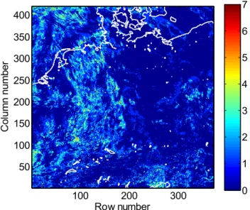
The scatterplot of the error of the adaptive temporal scheme versus the one of the persistence scheme (not shown) ex-hibits a cluster where the temporal scheme corrects both large and small errors of the persistence scheme almost per-fectly. Unfortunately, there is also a cluster where the tempo-ral scheme introduces errors where the persistence assump-tion was nearly perfect. The main cause of this cluster is that there are columns where the period between intrinsic calcu-lations is many hours. Figure 9 shows which columns were called how often from 12:00 until 13:00 UTC. Whereas in more convective regions up to seven calls are made, few in-trinsic calculations are performed in the cloud free region in the East. This results in larger errors in the East for the tem-poral scheme.
The temporal adaptive scheme is a clear improvement over a stand-alone regression algorithm. The bias errors of the stand-alone regression algorithm are large: 35 W m2(solar) and -3.6 W m−2(infrared). In the adaptive scheme, they are only 6 W m−2 (solar) and −0.3 W m−2 (infrared). The re-gression algorithm was developed based on spatial analysis data. However, it is utilised to predict temporal changes. The scatterplot of the difference between the surface net flux at 12:00 and 12:30 UTC versus the true difference from the δ-two-stream scheme (not shown) has an explained variance (r2) of 69% in the solar regimes and 66% in the infrared.
5.3.1 Modified schemes
To investigate how important which part of the adaptive tem-poral scheme is, three variations of the scheme were devel-oped. The errors and biases of the standard scheme and these three variations are presented in Table 3, under the heading “adaptive temporal scheme”. The scheme marked “perturba-tion only” calls the intrinsic calcula“perturba-tion at the full hours, i.e. no adaptive selection is performed. For the time steps be-tween the hours, the perturbation scheme is applied just as in the standard scheme. This perturbation-only scheme per-forms almost as well as the standard scheme; the RMS solar error is only 2 Wm−2larger, the RMS infrared error even a
0 10 20 30 40 50 -0.5 0 0.5 1 1.5 2 2.5x 10 6 11.1 km 6.66 km 5.08 km Spatial lag [km] (a) 0 10 20 30 40 50 -2 0 2 4 6 8 10x 10 4 12.8 km 12.1 km 5.22 km Spatial lag [km] (b) Persistence Temporal Spatial
Fig. 7. The covariance functions of the errors in the solar (a) and infrared (b) surface net flux. It quantifies the structure of the error fields
shown in Figs. 3 and 4 and demonstrates that the errors and the correlation length of the persistence scheme (red line) are larger compared to the temporal perturbation (blue long dashes) and the spatial local-search scheme (green short dashes).
0.4
0.6
0.8
1
1.2
40
60
80
100
Rel. no. intrinsic calculations
-2
(a)
3x3
4x4
5x5
6x6
0.4
0.6
0.8
1
1.2
10
15
20
Rel. no. intrinsic calculations
-2
(b)
Persistence Temporal Spatial - optimal Spatial - fixed
Fig. 8. The RMS error in the solar (a) and infrared (b) net radiative flux as a function of the relative number of intrinsic calculations. The
number of calls to the δ-two-stream scheme is normalised by the number of calculations for the full field once per hour. The blue dotted line denotes the spatial scheme with the weights of the standard scheme. The red line designates the spatial scheme where the weights are optimised for each number of function calls.
little smaller. This demonstrates the importance of the per-turbation technique.
The second variation indicated as “selection only”, utilises the regression scheme to select the columns where the in-trinsic parameterisation should be called, just as in the stan-dard scheme. Between the calls, the radiative perturbation is kept constant, i.e. the perturbation algorithm is not employed. This scheme has significantly larger errors than the standard temporal scheme, but still the errors are much less than the persistence scheme. Thus, the selection method by itself is important.
A selection algorithm can theoretically be even more im-portant. This can be seen in the scheme denoted “selection (true worst)”. This variation operates like the standard tem-poral scheme, except that the selection is not made by the regression algorithm, but by the δ-two-stream scheme itself. This purely theoretical scheme simulates a selection algo-rithm that is able to perfectly select those columns with the largest deviation in the surface net radiative flux. This last variation is clearly better than the standard scheme.
Row number 100 200 300 50 100 150 200 250 300 350 400 0 1 2 3 4 5 6 7
Fig. 9. Number of calls to the δ-two-stream scheme of the temporal
perturbation scheme from 12:00 to 13:00 UTC.
5.4 Spatial local-search scheme
The size of the search region and the weights of the spatial scheme have been optimised using a simplex optimisation algorithm (Nelder and Mead, 1965). This efficient algorithm requires a smooth function with only one global maximum. Because the cost function is somewhat noisy, sometimes a local maximum near the global maximum is found. Because of this, an additional manual optimisation is performed.
We have minimised the difference in solar net flux between the adaptive scheme and the δ-two-stream calculation com-puted on every column for 12:30 UTC. A similar minimisa-tion of the average error on the fields 2 and 4 h before and after 12:30 UTC resulted in an RMS error that was only 1% larger. Minimising for a small Alpine region (with a much smaller correlation length) produced an RMS error that was 2% larger. The size of the search region and the weights thus seem to be reasonably universal.
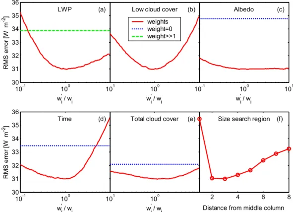
Figure 10 gives an idea of the robustness of the algorithm. Changing the individual weights up or down by a factor of 10 decreases the accuracy (RMS error of the solar net flux) of the algorithm by 5 W m−2 at maximum. Changing the size of the search region between 5×5 (maximum distance from the centre d=2) and 17×17 (d=8) has little influence as well. Larger search regions perform less well because of the increasing chance that columns with very different vertical profiles of their optical properties can have similar integrated properties. The small difference between the accuracy for d=2 and d=3 might not warrant the additional computational costs. It is interesting to note that a spatial parameterisa-tion scheme that would be based on the similarity in LWP would be able to achieve an accuracy of 33.9 W m−2 in the solar regime; see the green line in Fig 10a. Such a scheme
would thus only be 2.9 W m−2less accurate than the standard scheme.
Besides the mentioned four integrated parameters (Eq. 3) to estimate the similarity of two columns, we tried a number of additional parameters. The inclusion of a term for the hor-izontal distance brings an improvement of 0.7 W m−2and is thus much less important than the similar term for the time difference. The inclusion of a term for the cloud boundaries, such as cloud base height or temperature, is challenging as cloud boundaries are inherently not well defined and many columns do not contain clouds at all. Simply defining the cloud base as the first level with any cloud and setting cloud base height to zero for columns with no clouds, this term im-proves the accuracy by 0.9 W m−2. In an earlier version of this scheme, the influence of the ice water path was tested and it was found to contribute less than 1 W m−2. In an oper-ational scheme these small contributions may be worthwhile, but in this proof-of-concept study we have chosen to keep the scheme as simple as possible.
6 Discussion
In this discussion section, we will first discuss the common results of both schemes (Sect. 6.1), before we will discuss the temporal (Sect. 6.2) and the spatial scheme (Sect. 6.3) individually. Based on the current results, ideas for improve-ments of these two schemes will also be given. Expecting that adaptive schemes can also be developed for other small-scale processes, the final subsection discusses more long-term perspectives for adaptive parameterisation schemes. 6.1 Both adaptive schemes
6.1.1 Efficiency
An attractive feature of the adaptive schemes is that their ac-curacy decreases slowly with a reduction in the number of intrinsic calculations; see Fig. 8. Especially, the accuracy of the adaptive schemes decreases much slower than for the per-sistence scheme. Adaptive schemes thus provide a much bet-ter trade-off between the accuracy and the number of intrin-sic calculations. This property will make dynamical models more flexible. For instance, for long integrations, less accu-racy can be chosen, whereas for shorter runs a higher num-ber of intrinsic calculations can be selected. Furthermore, the computational resources saved by the reduction in the num-ber of calls can be utilised for parameterisation schemes re-solving more physical processes.
Both adaptive schemes achieved considerable improve-ments in accuracy with the same or a smaller number of calls to the δ-two-stream scheme. The improvement is partially that large because the 1-h persistence assumption leads to large errors at the high model resolution of the COSMO-DE. At 2.8 km resolution, it is advantageous to employ a radiative transfer parameterisation that works with a coarser model
10-1 100 101 30 31 32 33 34 35 36 LWP wi' / wi -2 (a) 100 Low cloud cover
wi' / wi (b) weights weight=0 weight>>1 10-1 100 101 Albedo wi' / wi (c) 10-1 100 101 30 31 32 33 34 35 36 Time wi' / wi -2 (d) 100 Total cloud cover
wi' / wi
(e)
2 4 6 8
Size search region
Distance from middle column (f)
Fig. 10. The robustness of the spatial local-search scheme to changes in the weighting factors and in the size of the search region, as illustrated
by the RMS error of the solar surface net flux. The weighting factors are for (a) liquid water path, (b) cloud cover of low clouds, (c) surface albedo, (d) the time difference and (e) the total cloud cover. The weighting factors (w′i) are varied by a factor ten up and down relative to
the standard weighting factors (wi). The horizontal lines indicate the accuracy of an algorithm without this parameter, i.e. w
′
i=0, or with this
parameter dominating, i.e. wi′=1012wi. These lines are omitted for clarity if they are outside the range. Panel (f) shows the influence of the
size of the square search region on the accuracy; on the x-axis is the maximum search distance (d) from the centre in columns.
grid than the dynamical resolution. Such a coarse-grained parameterisation can also be part of an adaptive scheme; in such a case, the accuracy gains will likely be more modest. 6.1.2 Dynamical effects
Even if the accuracy had stayed the same, the schemes would still have the advantage of being able to utilise a short time step at little computational cost. This smaller time step al-lows to model feedbacks on shorter time scales and reduces physical inconsistencies that can be caused by the persistence assumption. An example of the latter is that the persistence assumption leads to an increase in situations where rain is combined with strong insolation. Such physical inconsisten-cies will be discussed in more detail in an upcoming study.
The correlation length of the error fields is longest for the persistence assumption and shortest for the adaptive spatial scheme. From the work on stochastic parameterisations, it is known that disturbances with a short correlation time and length have little dynamical influence on the dynamics of the models (Buizza et al., 1999; Theis, 2005). Thus, even if the RMS errors of the adaptive schemes had been similar, these
errors would probably be dynamically less problematic as the correlated errors of the persistence assumption.
In this work, the focus is on the surface net radiative flux because the strongest feedbacks are expected here. An ex-tension to the full vertical profile is technically trivial for the spatial local-search scheme, but it will need to be demon-strated whether the gains are similar. The temporal scheme can be extended to atmospheric heating rates as well, but care will have to be taken to assure energy conservation.
6.1.3 Future radiation schemes
In the presented application to radiative transfer, the spatial scheme clearly performed better than the temporal scheme. Still we wanted to present both schemes because this result could be reversed for parameterisations of other processes or models and/or on different scales. Furthermore, a combined scheme may be interesting, as the strength of the perturbation algorithm is the correction of temporal development, and the strong point of the local-search method is the adjustment for spatial developments.
Atmospheric variables are characterised by power (vari-ance) spectra that decrease monotonically towards small scales. Thus, with increasing number of grid points of NWP and climate models, the atmospheric variables in adjacent grid boxes will become ever stronger correlated. Conse-quently, almost the same parameterisation is calculated in ad-jacent grid boxes or columns and the improvement in compu-tational efficiency of adaptive over conventional schemes can be expected to become larger in future. Assuming that the relevant atmospheric variables follow a power-law (fractal) power spectrum, only the number of grid points is relevant, not the model resolution itself. Even if the fractal approx-imation is only partially valid, we conjecture that adaptive techniques are not only useful for NWP, but also for climate models. Climate models likely suffer less from persistence errors, the emphasis would thus be on the improvement of the computational efficiency.
6.2 Temporal perturbation scheme
This first temporal perturbation scheme produced much bet-ter results than the scheme based on the persistence assump-tion. An artificial neural network is expected to be able to reproduce the training dataset more accurately than the mul-tivariate regression algorithm, as radiative transfer is highly nonlinear. This may also lead to an improvement of the ac-curacy of the full temporal scheme. A simple process-based parameterisation, e.g. Niemela et al. (2001a, 2001b), may also be a useful substitute for the regression algorithm.
In Sect. 5.3, we showed that the selection – of the columns for which the δ-two-stream scheme is called – based on the true largest changes in the irradiance (as calculated by the δ-two-stream parameterisation itself), leads to a large improve-ment in accuracy. Of course, this is not a practicable selec-tion algorithm, but it does show that there is still room for improvements. Even if there is no guarantee that a simple al-gorithm is able to achieve better results, it does suggest that it would be worthwhile to try to find a smarter algorithm.
The next step towards developing an operational version of the adaptive temporal scheme is the training of the regres-sion algorithm on a larger dataset that includes cloud fields throughout the day and year. At the moment, the scheme produces biases at times other than 12:00 UTC. Preliminary results show that these biases are reduced considerably by training the algorithm on full day model runs.
6.3 Spatial local-search scheme
In this case study, the spatial scheme clearly gives the best re-sults: the RMS error and its correlation length are the small-est. Improvements may be expected by a combination of the spatial scheme and the temporal scheme. The regression al-gorithm could play three roles: selection of the grid boxes for the intrinsic calculations, the determination of the most
similar local column and the calculation of an additional per-turbation term.
The order in which the intrinsic calculations are called is determined by hand to optimise the distance between con-secutive columns and to spread the intrinsic calculations ho-mogeneously. Modest gains may be possible by developing a method to compute optimised patterns automatically. Es-pecially for larger regions, the development of the patterns by hand is a difficult task and likely to be suboptimal.
For this application, the generalisation was optimised for a small RMS error for the solar fluxes. In a climate model, it may be more appropriate to optimise for biases in the radia-tive budget as well.
6.4 Future intrinsic parameterisations
Many parameterisations are calibrated using the results of more detailed models or tuned to improve model predictions. This inherently means that part of such a parameterisation is adjusted to climatological conditions. For instance, in case of the radiative transfer parameterisation of the COSMO model, the assumptions regarding effective radius and subgrid-scale cloud structures are climatological. One could state that in an adaptive scheme the extrinsic parameterisation is tuned dynamically during the model run as it adapts to the intrinsic calculations; the bias of the stand-alone regression algorithm is much larger than that of the adaptive scheme employing this scheme. The goal of adaptive parameterisation schemes is to enable the use of intrinsic parameterisations that resolve more small-scale processes and thus rely less on climatolog-ical assumptions. In this paper, we have not yet reached this goal, as the original radiative transfer parameterisation is still employed.
A modelling methodology that shares our aim of making parameterisation more physical is the super-parameterisation or Multi-Model Framework (MMF) (Grabowski, 2001; Ran-dall et al., 2003a). This framework tackles the problem of modelling subscale structures head-on, by nesting 2D cloud-resolving models (CRM) into every column of a climate model. This methodology offers the hope of being able to understand the cloud feedback in climate change. However, it has two main disadvantages. Firstly, it is computationally very expensive and secondly, it is questionable if a 2D CRM with 4-km resolution can provide realistic cloud structures. Within the adaptive approach, one would drastically reduce the number of CRMs utilised in the MMF and try to “cal-ibrate” the existing parameterisations based on a compari-son with the CRMs. Due to the reduction in the number of CRMs, these could be 3-dimensional with a higher resolu-tion. This is likely important for cloud structure and convec-tion.
An adaptive scheme based on high-resolution CRM results would not only be useful for studying the cloud feedback effect, but may also be a way to design atmospheric mod-els with consistent physics. However, it seems prudent to
first gain some experience with adaptive parameterisations for various individual parameterisations.
The δ-two-stream scheme of the COSMO model multi-plies the cloud water content with a multiplicative factor of one-half to account for small-scale cloud structure. Our tem-poral perturbation scheme adds an additive constant to its output based on the intrinsic calculation. Applying such ad-ditive constants or multiplicative factors to the input or to the output is a first simple way to calibrate extrinsic pa-rameterisations based upon the intrinsic calculations. The smarter and more adaptive the generalisations are, the less often computationally expensive intrinsic parameterisations will be needed.
The example schemes in this paper had one generalisa-tion and one intrinsic parameterisageneralisa-tion. However, it might be worthwhile to employ multiple steps. For example, a compu-tationally expensive version of the Monte Carlo Independent Column Approximation (McICA) parameterisation (Barker et al., 2002; Pincus et al., 2003) with a larger than typi-cal number of subcolumns could be utilised to typi-calibrate a conventional δ-two-stream scheme, which would calibrate a generalisation.
7 Summary and outlook
This paper presented two adaptive parameterisation schemes for radiative transfer in a limited area model, the COSMO model. The first method, a temporal perturbation scheme starts by computing the full radiation field with a δ-two-stream scheme. Then it regularly calculates the changes with a simple regression scheme. Large (local) biases typ-ical for regression schemes are avoided because the regres-sion algorithm is only employed to calculate changes. Fur-thermore, the regression method is employed to select the columns where the δ-two-stream scheme is called. The sec-ond method is based on a local-search algorithm. Every ra-diation time step of 5 min, it calls the δ-two-stream scheme in a small number of columns. The radiative tendencies of the other columns are determined by a local-search algorithm that searches for a column with similar radiative properties for which the tendencies are already known. The similarity is determined by a weighted index taking account of the dif-ferences in liquid water path, cloud cover, and albedo, and the time passed since the δ-two-stream scheme was called.
Both schemes are judged against a scheme where the δ-two-stream scheme is called every full hour for all columns and the radiative quantities are assumed to remain constant between those calls. The schemes are compared using a case study, the 19 September 2001 at 12:30 UTC. For these fields the persistence assumption results in a RMS error in the so-lar net radiative flux at the surface of 77 W m2and an error in the infrared net flux of 15 W m−2. The error of the adaptive schemes is much smaller. The temporal perturbation scheme has a RMS error in the solar net flux of 43 W m−2, and in
the infrared net flux of 9.1 W m−2. The spatial local-search scheme produces an error in the solar net flux of 31 W m−2 and in the infrared net flux of 6.3 W m−2. Furthermore, the correlation length of the error fields of the adaptive schemes is smaller than that resulting from the persistence assump-tion.
The schemes described in the previous paragraph all made about the same number of calls to the δ-two-stream radia-tive transfer scheme. An important quality of the adap-tive schemes is, however, that significant reductions in the number of calls to the δ-two-stream scheme are possible with only small decreases in their accuracy. For example, calling the δ-two-stream scheme once every three hours in-creases the error of the persistence scheme to 107 W m−2. However, the error of the temporal perturbation scheme is only increased to 52 W m−2, and of the spatial local-search scheme to 34 W m−2. This increase in computational effi-ciency can be utilised to employ more complex parameterisa-tion schemes that resolve more subscale processes or model them in more detail.
The calculations in this work are performed using the output from the COSMO model. We are now working on parallelising and implementing the schemes in the COSMO model. In an upcoming paper, we plan to report on a num-ber of full day case studies with the new adaptive schemes and will especially focus on the improvements in the physi-cal consistency of the model due to the adaptive methods.
In Sect. 6.4, a number of ideas were presented on adaptive parameterisation for cloud processes. We presume that adap-tive parameterisation schemes can be relevant to many dif-ferent subscale processes and dynamical models. The main requirement is that the physical quantities underlying the pro-cesses are correlated in time or space.
Acknowledgements. We are grateful to H. Barker, T. Reinhardt,
B. Ritter, M. Rotach, M. Schr¨oder and D. Wilson for many useful comments that considerably improved the presentation. Further-more, we would like to thank M. Schr¨oder (present affiliation EUMETSAT) for the analysis of the correlation length of the liquid water path of MODIS. Part of this work was performed in the 4D-Clouds project, which was sponsored by the German ministry of research (BMBF) in the AFO2000 program. The thought-provoking book by D. Hofstadter (1995) should be acknowledged as being an important starting point for the ideas on adaptive parameterisations.
Edited by: J. Quaas
References
Baldauf, M., F¨orstner, J., Klink, S., Reinhardt, T., Schraff, C., Seifert, A., and Stephan, K.: Kurze Beschreibung des Lokal-Modells K¨urzestfrist LMK und seiner Datenbanken auf dem Datenserver des DWD, Stand 27.10.2006, DWD, Offenbach, Germany, 2006.
Barker, H. W., Pincus, R., and Morcrette, J.-J.: The Monte Carlo independent column approximation: application within large-scale models, Proc. GCSS-ARM Workshop on the Representa-tion of Cloud Systems in Large-Scale Models, Kananaskis, Al-berta, Canada, 20–24 May, 2002.
Buizza, R., Miller, M., and Palmer, T. N.: Stochastic representa-tion of model uncertainties in the ECMWF ensemble predicrepresenta-tion system, Q. J. Roy. Meteor. Soc., 125, 2887–2908, 1999. Chevallier, F., Ch´eruy, F., Scott, N. A., and Ch´edin, A.: A neural
network approach for a fast and accurate computation of a long-wave radiative budget, J. Appl. Meteorol., 37, 1385–1397, 1998. Chevallier, F., Morcrette, J.-J., Ch´eruy, F., and Scott, N. A.: Use of a neural-networkbased long-wave radiative-transfer scheme in the ECMWF atmospheric model, Q. J. Roy. Meteor. Soc., 126, 761– 776, 2000.
Collins, W. D., Rasch, P. J., Boville, B. A., et al.: Descrip-tion of the NCAR Community Atmosphere Model (CAM 3.0). NCAR Technical note, National Center for Atmospheric Re-search, Boulder, Colorado, http://www.ccsm.ucar.edu/models/ atm-cam/, 2004.
Davis, A. B., Marshak, A., Gerber, H., and Wiscombe, W. J.: Hor-izontal structure of marine boundary-layer clouds from cm- to km-scales, J. Geophys. Res., D104, 6123–6144, 1999.
Gagnon, J. S., Lovejoy, S., and Schertzer, D.: Multifractal earth topography, Nonlin. Processes Geophys., 13, 541–570, 2006, http://www.nonlin-processes-geophys.net/13/541/2006/. Grabowski, W. W.: Coupling cloud processes with the large-scale
dynamics using the Cloud-Resolving Convection Parameteriza-tion (CRCP), J. Atmos. Sci., 59, 978–997, 2001.
Geleyn, J.-F., Fournier, R., Hello, G., and Pristov, N.: A new “bracketing” technique for a flexible and economical computa-tion of thermal radiative fluxes, on the basis of the Net Exchange Rate (NER) formalism, WGNE Blue Book, 4-07, 2005. Green, J. S. A.: Division of radiative streams into internal transfer
and cooling to space, Q. J. Roy. Meteor. Soc., 93, 371–372, 1967. Hofstadter, D. R.: Fluid concepts and creative analogies, Basic
books, New York, 1995.
Kessler, E.: On the distribution and continuity of water substance in atmospheric circulations, Meteorological Monographs, 10(32), p. 84, 1969.
King, M. D., Tsay, S. C., Platnick, S. E., Wang, M., Liou, K.-N.: Cloud retrieval algorithms for MODIS: Optical thickness, effec-tive particle radius, and thermodynamic phase. Algorithm Theo-retical Basis Document ATBD-MOD-05, NASA, Goddard Space Flight Center, Greenbelt, Maryland, 1997.
Krasnopolski, V. M., Fox-Rabinovitz, M. S., and Chalikov, D. V.: New approach to calculation of atmospheric model physics: Ac-curate and fast neural network emulation of longwave radiation in a climate model, Mon. Weather Rev., 133, 1370–1383, 2005. Matsui, T., Leoncini, G., Pielke Sr., R. A., and Nair, U. S.: A new
paradigm for parameterization in atmospheric models: applica-tion to the new Fu-Liou radiaapplica-tion code, Colorado State Univer-sity, Dept. of Atmospheric Sci., paper no. 747, 2004.
Majewski, D., Lierman, D., Prohl, P., Ritter, B., Buchhold, M., Hanisch, T., Paul, G., Wergen, W., and Baumgardner, J.: The operational global icosahedral-hexagonal gridpoint model GME: Description and high-resolution tests, Mon. Weather Rev., 130, 319–338, 2002.
Meteo France: Book 1, Chapter 21: The radiation parameterization, In The Meso-NH scientific documentation, http://mesonh.aero. obs-mip.fr/mesonh, 2002.
Morcrette, J.-J.: On the effects of the temporal and spatial sampling of radiation fields on the ECMWF forecasts and analyses, Mon. Weather Rev., 128, 876–887, 2000.
Nelder, J. A. and Mead, R.: A simplex method for function mini-mization, Comput. J., 7, 308–313, 1965.
Niemela, S., Raisanen, P., and Savijarvi, H.: Comparison of surface radiative flux parameterizations – Part I: Longwave radiation, At-mos. Res., 58(1), 1–18, 2001a.
Niemela, S., Raisanen, P., and Savijarvi, H.: Comparison of surface radiative flux parameterizations – Part II, Shortwave radiation, Atmos. Res., 58(2), 141–154, 2001b.
Pincus, R., Barker, H. W., and Morcrette, J.-J.: A fast flexi-ble approximate technique of computing radiative transfer for inhomogeneous clouds, J. Geophys. Res., 108(D13), 4376, doi:10.1209/2002JD003322, 2003.
Pielke Sr., R. A., Matsui, T., Leoncini, G., Nobis, T., Nair, U. S., Lu, E., and Walko, R. L.: A new paradigm for parameterizations in numerical weather prediction and other atmospheric models, National Wea. Digest, 30, 93–99, 2005.
Randall, D., Khairoutdinov, A. M., Arakawa, A., and Grabowski, W. W.: Breaking the cloud parameterization deadlock, Bull. Am. Meteorol. Soc., 84, 1547–1564, 2003a.
Randall, D., Krueger, St., Bretherton, Ch., Curry, J., Duynkerke, P., Moncrieff, M., Ryan, B., Starr, D., Miller, M., Rossow, W., Tselioudis, G., and Wielicki B.: Confronting models with data: the GEWEX Cloud Systems Study, Bull. Am. Meteorol. Soc., 84(4), 455–469, 2003b.
Reinhardt, T. and Seifert, A.: A three-category ice scheme for LMK, COSMO Newsletter, no. 6, July, 115–120, 2006. Ritter, B. and Geleyn, J.-F.: A Comprehensive radiation scheme for
numerical weather prediction models with potential applications in climate simulations, Mon. Weather Rev., 120, 303–325, 1992. Sass, B. H., Rontu, L., and R¨ais¨anen, P.: HIRLAM-2 radia-tion scheme: Documentaradia-tion and tests, Rep. no. 16, SMHI, Norrk¨oping, Sweden, 1994.
Sch¨attler, U., Doms, G., and Schraff, C.: Description of the nonhydrostatic regional model (LM). Part VII: user’s guide, COSMO-Consortium for Small Scale Modelling, http://www. cosmo-model.org, 2005.
Steppler, J., Doms, G., Sch¨attler, U., Bitzer, H. W., Gassmann, A., Damrath, U., and Gregoric, G.: Meso-gamma scale forecasts us-ing the nonhydrostatic model LM, Meteorol. Atmos. Phys., 82, 75–96, 2003.
Theis, S.: Deriving probabilistic short-range forecasts from a deter-ministic high-resolution model, PhD thesis, University of Bonn, 2005.
Tiedtke, M.: A comprehensive mass flux scheme for cumulus pa-rameterisation in large-scale models, Mon. Weather Rev., 117, 1779–1799, 1989.
Und´en, P., Rontu, L., J¨arvinen, H., et al.: HIRLAM-5 scientific documentation, SMHI, Norrk¨oping, Sweden, 2002.
WCRP: Annual review of the World Climate Research Pro-gramme and report of the twenty-fifth session of the Joint Scientific Committee, http://www.wmo.ch/pages/prog/wcrp/pdf/ jsc25report.pdf, Moscow, Russian Federation, 1–6 March, 2004.