HAL Id: inria-00166791
https://hal.inria.fr/inria-00166791
Submitted on 9 Aug 2007
HAL is a multi-disciplinary open access
archive for the deposit and dissemination of
sci-entific research documents, whether they are
pub-lished or not. The documents may come from
teaching and research institutions in France or
abroad, or from public or private research centers.
L’archive ouverte pluridisciplinaire HAL, est
destinée au dépôt et à la diffusion de documents
scientifiques de niveau recherche, publiés ou non,
émanant des établissements d’enseignement et de
recherche français ou étrangers, des laboratoires
publics ou privés.
Mosaicing of Confocal Microscopic In Vivo Soft Tissue
Video Sequences
Tom Vercauteren, Aymeric Perchant, Xavier Pennec, Nicholas Ayache
To cite this version:
Tom Vercauteren, Aymeric Perchant, Xavier Pennec, Nicholas Ayache. Mosaicing of Confocal
Micro-scopic In Vivo Soft Tissue Video Sequences: Mosaicing of Confocal MicroMicro-scopic In Vivo Soft Tissue
Video Sequences. Medical Image Computing and Computer-Assisted Intervention, Oct 2005, Palm
Springs, United States. pp.753-760, �10.1007/11566465_93�. �inria-00166791�
Tissue Video Sequences
Tom Vercauteren1,2, Aymeric Perchant2, Xavier Pennec1, and Nicholas
Ayache1
1 Projet Epidaure, INRIA Sophia-Antipolis, France 2 Mauna Kea Technologies, 9 rue d’Enghien Paris, France
Abstract. Fibered confocal microscopy allows in vivo and in situ imag-ing with cellular resolution. The potentiality of this imagimag-ing modality is extended in this work by using video mosaicing techniques. Two novelties are introduced. A robust estimator based on statistics for Riemannian manifolds is developed to find a globally consistent mapping of the input frames to a common coordinate system. A mosaicing framework using an efficient scattered data fitting method is proposed in order to take into account the non-rigid deformations and the irregular sampling implied by in vivo fibered confocal microscopy. Results on 50 images of a live mouse colon demonstrate the effectiveness of the proposed method.
1
Introduction
Fibered confocal microscopy (FCM) is a potential tool for in vivo and in situ optical biopsy [1]. FCM is based on the principle of confocal microscopy which is the ability to reject light from out-of-focus planes and provide a clear in-focus image of a thin section within the sample. This optical sectioning property is what makes the confocal microscope ideal for imaging thick biological samples. The adaptation of a confocal microscope for in vivo and in situ imaging can be viewed as replacing a microscope objective by a probe of adequate length and diameter in order to be able to perform in situ imaging. For such purpose, a fiber bundle is used as the link between the scanning device and the microscope objective. After image processing of the FCM raw output, the available informa-tion is composed of a video sequence irregularly sampled in the space domain, each sampling point corresponding to a fiber center [1].
This imaging modality unveils the cellular structure of the observed tissue. The goal of this work is to enhance the possibilities offered by FCM by using image sequence mosaicing techniques in order to widen the field of view (FOV). Several possible applications are targeted. First of all, the rendering of wide-field micro-architectural information on a single image will help experts to interpret the acquired data. This representation will also make quantitative and statistical analysis possible on a wide field of view. Moreover, mosaicing for microscopic im-ages is a mean of filling the gap between scales and allows multiscale information fusion for probe positioning and multi-modality fusion.
2 Tom Vercauteren, Aymeric Perchant, Xavier Pennec, and Nicholas Ayache
Each frame of the input sequence is modeled as a deformed partial view of a ground truth 2D scene. The displacement of the fiber bundle probe across the tissue is described by a rigid motion. Due to the interaction of the contact probe with the soft tissue, a small non-rigid deformation appears on each input frame. Because of those non-linear deformations, and the irregular sampling of the input frames, classical video mosaicing techniques need to be adapted.
In Section 2, our mosaicing framework is described. The first main contribu-tion presented in Seccontribu-tion 3 is the use of Riemannian statistics to get a robust estimate of a set of mean rigid transformations from pairwise registrations re-sults. The second main contribution is proposed in Section 4 where we develop a mosaicing framework using an efficient scattered data fitting method well-suited for non-linear deformations and irregularly sampled inputs. Finally real experi-ments described in Section 5 demonstrate the effectiveness of our approach and show the significant image improvements obtained by using non-linear deforma-tions.
2
Problem Formulation and Mosaicing Method
The goal of many existing mosaicing algorithms is to estimate the reference-to-frame mappings and use these estimates to construct the mosaic [2]. Small residual misregistrations are then of little importance because the mosaic is reconstructed by segmenting the field into disjoint regions that use a single source image for the reconstruction [3,4]. Since our input frames are rather noisy, we would like to use all the available information to recover an approximation of the true underlying scene. We will therefore estimate the frame-to-reference transformations (instead of the usual reference-to-frame) and consider all the input sampling points as shifted sampling points of the mosaic. This has several advantages for our problem. First of all, this is really adapted to irregularly sampled input frames because we will always use the original sampling points and never interpolate the input data. This approach is also more consistent with a model of noise appearing on the observed frames rather than on the underlying truth. Finally in this framework, it will be possible to get a mosaic at a higher resolution than the input frames. The drawback is that we need an accurate estimate of the unknown transformations.
Let I be the unknown underlying truth and In be the observed frames. Our
algorithm makes use of the following observation model,
In(p) = I(fn(p)) + ǫn(p), ∀p ∈ Ωn, (1)
where ǫn(p) is a noise term, Ωn is the coordinate system associated with the
nth input frame and f
n : Ωn → Ω is the unknown frame-to-reference mapping
composed of a large rigid mapping rn and a small non-rigid deformation bn,
fn(p) = bn◦ rn(p). (2)
By making the reasonable assumption that consecutive frames are overlap-ping, an initial estimate of the global rigid transformations can be obtained by
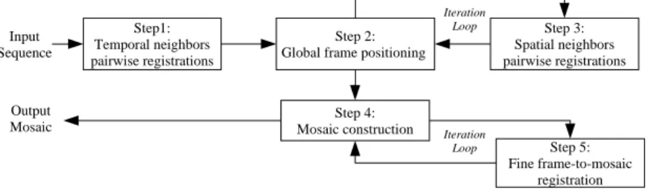
Step1: Temporal neighbors pairwise registrations
Step 2: Global frame positioning
Step 3: Spatial neighbors pairwise registrations Step 4: Mosaic construction Step 5: Fine frame-to-mosaic registration Input Sequence Output Mosaic Iteration Loop Iteration Loop
Fig. 1.Block diagram of the mosaicing algorithm
using an image registration technique to estimate the motion between the consec-utive frames. Global alignment is then obtained by composing the local motions. This initial estimate suffers from a well-known accumulation of error problem. Our algorithm depicted in Fig. 1 iteratively refines the global positioning by adding new pairwise rigid registration results to estimate the global parameters. Once a consistent set of rigid transformations is found, the algorithm constructs an initial mosaic by mapping all observed sampling points into the common ref-erence coordinate system and using an efficient scattered data fitting technique on this point cloud. The residual non-rigid deformations are finally taken into account by iteratively registering an input frame to the mosaic and updating the mosaic based on the new estimate of the frame-to-mosaic mapping.
3
Global Frame Positioning from Pairwise Registrations
The first task of our algorithm is to register pairs of overlapping input images under a rigid transformation assumption. For that purpose, we use a classical registration framework based on a similarity criterion optimization but any other technique (e.g. block matching framework [5], Mellin transform [3], feature-based registration [6] etc.) can be used. Let r(obs)j,i : Ωi → Ωj be the pairwise rigidregistration result between input frames i and j. This result is considered as a noisy observation of r−1
j ◦ ri. Based on the set of all available observations,
our algorithm looks for a globally consistent estimate of the global parameters [r1, . . . , rN]. This problem is addressed in [3] where a least-square solution is
given when linear transformations are considered. This technique cannot readily be adapted to rigid transformation. In [7], the authors propose a more general approach. Some chosen corner points are transformed through riand rj◦ r(obs)j,i .
The squared distance between the transformed points added to a regularization term is then minimized. These techniques are sensitive to outliers, and are either tailored to a specific type of transformation or need a somewhat ad hoc choice of points. In this paper statistics for Riemannian manifolds are used to provide a globally consistent and robust estimate of the global rigid transformation.
The computational cost of registering all input frames pairs is prohibitive and not all pairs of input frames are overlapping. It is therefore necessary to choose which pairs could provide informative registration results. For that purpose, we chose the topology refinement approach proposed in [7]. An initial guess of the
4 Tom Vercauteren, Aymeric Perchant, Xavier Pennec, and Nicholas Ayache
global parameters [r1, . . . , rN] is obtained by registering the consecutive frames,
the algorithm then iteratively chooses a next pair of input frames to register (thus providing a new observation r(obs)j,i ) and updates the global parameters
estimation. As we only consider the pairwise registration results as noisy obser-vations, we need many of them. In order to minimize the computational cost of those numerous registrations, we use a multiresolution registration technique using a Gaussian image pyramid that stops at a coarse level of the optimization. Given the set of all available pairwise registration results Θ, we need to estimate the true transformations. A sound choice is to consider a least-square approach. However the space of rigid transformations is not a vector space but rather a Lie group that can be considered as a Riemannian manifold. Classical notions using distances are therefore not trivial to generalize. In what follows, we provide an extension of the Mahalanobis distance for Riemannian manifolds [8] and propose an optimization algorithm to find the least-square estimate. Let r be an element of the 2D rigid transformations Riemannian manifold. From the theory of Riemannian manifolds, the vector V(r) representing r by its angle α(r) ∈ [−π, π] and translation components tx(r), ty(r) can be considered as a
mapping of the transformation r onto the vector space defined by the tangent space at the identity point Id of the manifold. This tangent space will be denoted as Id-tangent space. By using the canonical left-invariant Riemannian metric for rigid transformations, the distance of r to the identity is defined as the norm of the representation V(r) in the Id-tangent space, dist(r, Id) = ||V(r)||. The distance between two transformations is given by
dist(ra, rb) = dist(r−1b ◦ ra, Id) = ||V(r−1b ◦ ra)||. (3)
Using this distance, it is possible to define a generalized mean for a random transformation r, the Fr´echet mean Ef[r] = arg minrfE[dist(rf, r)
2]. If e is a
random error whose Fr´echet mean is the identity, its covariance matrix is simply defined as Σee = E[V(e)V(e)T]. The squared Mahalanobis distance between e
and the identity is given by µ2(e, Id) = V(e)TΣ−1
eeV(e). We now have the tools
to derive the global parameters estimator. The observation model is given by r(obs)j,i = r
−1
j ◦ ri◦ e(obs)j,i , where e (obs)
j,i is a random error whose Fr´echet mean is
assumed to be the identity and whose covariance matrix is Σee. An estimate
of [r1, . . . , rN] is given by the set of transformations that minimizes the total
Mahalanobis distance:
[ˆr1, . . . , ˆrN] = arg min [r1,...,rN]
X
(i,j)∈Θ
µ2(e(obs)j,i , Id) (4)
This equation does not admit a closed form solution but an efficient optimiza-tion method can be designed by a simple modificaoptimiza-tion of a usual non-linear least square optimizer such as the Gauss-Newton descent. The Riemannian struc-ture of the transformation space is taken into account by adapting the intrinsic geodesic gradient descent in [8]. The idea is to walk towards an optimum by a series of steps taken along a geodesic of the manifold rather than walking in the tangent vector space. Let r(t)be an estimate of a rigid transformation r at step
t, the intrinsic geodesic walking is achieved by finding a direction δr(t) and a
step length λ for the following update equation in the Id-tangent space: V(r(t+1)) = V(r(t)◦ λδr(t)). (5)
By contrast, if a usual optimization routine on the Id-tangent space is used, we get a walking direction ∆V(t) such that the update would be
V(r(t+1)) = V(r(t)) + λ∆V(t). (6)
Using (6) directly can be problematic because we are not assured to remain on the manifold. It is however possible to combine the power of intrinsic geodesic walking and the ease of use of classical optimization routine by mapping a walk-ing direction found in the Id-tangent space onto the manifold. For that purpose, a first order Taylor expansion of (5) around the identity is used:
V(r(t)◦ λδr(t)) = V(r(t)) + λJL(r(t)) · V(δr(t)) + O(λ2), (7)
where JL(r) = ∂V(r ◦ s)/∂V(s)|s=Id. By identifying (6) and (7), we see that
∆V(t)= JL(r(t)) · V(δr(t)). The walking direction in the manifold is thus
V(δr(t)) = JL(r(t))−1· ∆V(t). (8)
Within this general framework, several improvements can easily be added. The terms of the cost function can be weighted by some confidence measure, ro-bust estimation techniques such as M-estimators can be used to discard outliers, the noise variance can be re-estimated based on the measurements etc. We are now able to get robust and globally consistent estimates of the rigid transforma-tions which we use as initial estimates of the complete global transformatransforma-tions [f1, . . . , fN]. The resulting mosaics in Fig. 2(a) show an accurate global
position-ing of the input frames that is robust to erroneous pairwise registrations.
4
Frame to Mosaic Fine Registration
Once a globally consistent mosaic has been constructed, it is possible to make a fine multi-image registration by iteratively registering each input frame to the mosaic and updating the mosaic. The mosaicing problem can be written as an optimization problem over the unknown underlying image I and the unknown transformations [f1, . . . , fN] of the following multi-image criterion,
S(f1, . . . , fN, I) =PN
n=1S(In, I ◦fn), where S(Ia, Ib) is a usual pairwise
similar-ity criterion between the two images Ia and Ib. With this framework our mosaic
refinement procedure can be seen as an alternate optimization scheme.
We divide the fine frame-to-mosaic registrations into two loops of increasing model complexity. First we refine the global rigid mappings. Then, in order to account for the small non-rigid deformations, the residual deformation fields [b1, . . . , bN] are modeled by using B-splines tensor products on a predefined grid.
6 Tom Vercauteren, Aymeric Perchant, Xavier Pennec, and Nicholas Ayache
This framework can easily be extended to use any other non-rigid registration methods using landmarks-based schemes or more accurate deformation models. This iterative mosaic refinement scheme requires a new mosaic construction at each iteration. It is therefore necessary to use a very efficient reconstruction algorithm. Furthermore, since we want to register input frames with the mo-saic, the reconstruction needs to be smooth enough for the registration not to be trapped in a local minimum but detailed enough for the registration to be accurate. Once an estimate ˆfn of fn is available, we get a point cloud composed
of all transformed sampling points from all the input frames
{(pk, ik)} = {( ˆfn(p), In(p))|p ∈ Ωns, n ∈ [0, . . . , N ]}, (9)
where Ωs
nis the set of sampling points in the input frame n. The usual algorithms
for scattered data approximation do not simultaneously meet the requirements of efficiency, and control over the smoothness of the approximation. In the sequel we develop our second main contribution which is an efficient scattered data fitting algorithm that allow a control over the smoothness of the reconstruction. The main idea is to get an approximation of the underlying function by using a method close to Shepard interpolations. The value associated with a point in Ω is a weighted average of the nearby sampled values,
ˆ I(p) =X k wk(p)ik= X k hk(p) P lhl(p) ik. (10)
The usual choice is to take weights that are the inverse of the distance, hk(p) =
dist(p, pk)−1. In such a case we get a true interpolation [9]. An approximation is
obtained if a bounded weighting function hk(p) is chosen. We choose a Gaussian
weight hk(p) = G(p−pk) ∝ exp(−||p − pk||2/2σ2a) and thus (10) can be rewritten
as ˆ I(p) = P kikG(p − pk) P kG(p − pk) = [G ⋆ P kikδpk](p) [G ⋆Pkδpk](p) , (11)
where δpkis a Dirac distribution centered at pk. This scattered data
approxima-tion technique requires only two Gaussian filtering and one division and is thus very efficient. The smoothness is controlled by the variance σ2
a of the Gaussian
kernel. Thanks to this approximation method, we obtain a mosaic that is sharper and smoother than the original input frames as demonstrated in Section 5.
5
Results
In the field of colon cancer research, the development of methods to enable reliable and early detection of tumors is a major goal. In the colon, changes in crypt morphology are known to be early indicators of cancer development. The crypts that undergo these morphological changes are referred to as Aberrant Crypt Foci (ACF) and they can develop into cancerous lesions. Compared to the standard methods of ACF screening, fluorescence FCM enables the operator to see the lesions in real-time and to make an almost immediate evaluation.
However, in many cases the limited field of view restricts the confidence that the operator has in the ACF counting. By offering an extended field of view, mosaicing techniques can be an answer to this restriction.
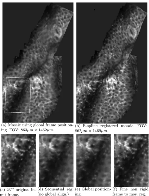
(a) Mosaic using global frame position-ing. FOV: 863µm × 1462µm.
(b) B-spline registered mosaic. FOV: 862µm × 1469µm.
(c) 23rd
original in-put frame.
(d) Sequential reg. (no global align.)
(e) Global position-ing.
(f) Fine non rigid frame to mos. reg. Fig. 2. Mosaic of 50 live mouse colon images (Fluorescence FCM). The zone corre-sponding to the 23rd
input frame is detailed for different steps of the algorithm. FOV one input: 303µm × 425µm. Images are courtesy of Danijela Vignjevic, Sylvie Robine, Daniel Louvard, Institut Curie, Paris, France
8 Tom Vercauteren, Aymeric Perchant, Xavier Pennec, and Nicholas Ayache
The effectiveness of the proposed algorithm is shown on a sequence that has been acquired in-vivo on a mouse colon stained by acriflavine at 0,001%. The mouse was treated with azoxymethane (AOM) to induce a colon cancer. As shown in fig.2(b), our algorithm allows for a simultaneous visualization of normal crypts and ACFs.
The global frame positioning mosaicing took approximately 1 min on a 2GHz P4 and 12 min if the non-rigid deformations are compensated. The imaged tissue is really soft and non-linear deformations occur. Figure 2(b) illustrates the gain we obtain by taking into account those non-rigid deformations. Some details are lost if we only use rigid deformations and appear again on our final mosaic. The results shown here prove the feasibility of mosaicing for in-vivo soft-tissue mi-croscopy. Current work is dedicated to the validation of the proposed approach.
6
Conclusion
The problem of video mosaicing for in-vivo soft tissue confocal microscopy has been explored in this paper. A fully automatic robust approach based on Rie-mannian statistics and efficient scattered data fitting techniques was proposed. The results shown for two different imaging modalities are promising and en-courage the application of the proposed method for qualitative and quantitative studies on the mosaics.
References
1. G. Goualher, A. Perchant, M. Genet, C. Cave, B. Viellerobe, F. Berier, B. Abrat, and N. Ayache, “Towards optical biopsies with an integrated fibered confocal fluo-rescence microscope,” in Proc. of MICCAI’04, 2004, pp. 761–768.
2. M. Irani, P. Anandan, and S. Hsu, “Mosaic based representations of video sequences and their applications,” in Proc. ICCV’95,, June 1995, pp. 605–611.
3. J. Davis, “Mosaics of scenes with moving objects,” in Proc. CVPR’98, 1998, pp. 354–360.
4. S. Peleg, B. Rousso, A. Rav-Acha, and A. Zomet, “Mosaicing on adaptive mani-folds,” IEEE Trans. Pattern Anal. Machine Intell., vol. 22, no. 10, pp. 1144–1154, Oct. 2000.
5. S. Ourselin, A. Roche, S. Prima, and N. Ayache, “Block matching: A general frame-work to improve robustness of rigid registration of medical images,” in Proc. MIC-CAI’00, 2000, pp. 557–566.
6. A. Can, C. V. Stewart, B. Roysam, and H. L. Tanenbaum, “A feature-based tech-nique for joint linear estimation of high-order image-to-mosaic transformations: Mosaicing the curved human retina,” IEEE Trans. Pattern Anal. Machine Intell., vol. 24, no. 3, pp. 412–419, Mar. 2004.
7. H. S. Sawhney, S. Hsu, and R. Kumar, “Robust video mosaicing through topology inference and local to global alignment,” in Proc. ECCV’98, vol. 2, 1998, pp. 103– 119.
8. X. Pennec, “Probabilities and statistics on Riemannian manifolds: Basic tools for geometric measurements,” in Proc. NSIP’99, vol. 1, 1999, pp. 194–198.
9. I. Amidror, “Scattered data interpolation methods for electronic imaging systems: a survey,” J. Electron. Imaging, vol. 11, no. 2, pp. 157–176, Apr. 2002.