On the identification of cohesive zone model for curved crack in mortar

HAL Id: hal-02555911

https://hal.archives-ouvertes.fr/hal-02555911

HAL is a multi-disciplinary open access

archive for the deposit and dissemination of sci-entific research documents, whether they are pub-lished or not. The documents may come from teaching and research institutions in France or abroad, or from public or private research centers.

L’archive ouverte pluridisciplinaire HAL, est destinée au dépôt et à la diffusion de documents scientifiques de niveau recherche, publiés ou non, émanant des établissements d’enseignement et de recherche français ou étrangers, des laboratoires publics ou privés.

crack in mortar

R Vargas, A Tsitova, F. Bernachy-Barbe, B Bary, R B Canto, François Hild

To cite this version:

R Vargas, A Tsitova, F. Bernachy-Barbe, B Bary, R B Canto, et al.. On the identification of co-hesive zone model for curved crack in mortar. Strain, Wiley-Blackwell, 2020, 56 (6), pp.e12364. �10.1111/str.12364�. �hal-02555911�

DOI: xxx/xxxx

RESEARCH PAPER

On the identification of cohesive zone model for curved crack in

mortar

R. Vargas

_{| A. Tsitova}

_{| F. Bernachy-Barbe}

_{| B. Bary}

_{| R.B. Canto}

_{| F. Hild*}

1_{Graduate Program in Materials Science and}

Engineering (PPGCEM), Federal University of São Carlos (UFSCar), São Carlos, Brazil

2_{Den-Service d’Etude du Comportement des}

Radionucléides (SECR), CEA, Université Paris-Saclay, Gif-sur-Yvette, France

3_{Université Paris-Saclay, ENS Paris-Saclay,}

CNRS, LMT - Laboratoire de Mécanique et Technologie, Cachan, France

4_{Federal University of São Carlos (UFSCar),}

Department of Materials Engineering (DEMa), São Carlos, Brazil

Correspondence

*François Hild

Email: francois.hild@ens-paris-saclay.fr

Summary

This paper proposes an approach to defining the path of a curved crack in a single edge notched specimen with gray level residuals extracted from digital image cor-relation, followed by the calibration of the parameters of a cohesive zone model. Only the experimental force is used in the cost function minimized via finite element model updating. The displacement and gray level residual fields allow for the vali-dation of the calibrated parameters. Last, the results are confronted with those given by a straight crack to highlight the benefits of accounting for the actual crack path.

KEYWORDS:

Calibration, digital image correlation (DIC), finite element model updating (FEMU), gray level residuals

1

INTRODUCTION

The safety of double wall Concrete Containment Buildings (CCB) that are widely used in the French nuclear industry primarily depends on the integrity of concrete. The delayed deformations of concrete induced by creep and shrinkage cause microcracking and a loss of pre-stress that is the major factor in reducing the leak tightness of the CCB internal wall in accidental conditions [12]. Creep of concrete is a complex phenomenon and its rate depends on several factors among which microcracking itself is of major significance [6], which is also crucial for other analyses (e.g., fracture mechanics). To improve the predictive capabilities of models describing the mechanical response of concrete, the coupling of damage and viscous behavior is currently studied at the mesoscale, and starts with an accurate modeling of the fracture behavior. The latter is the focus of the present paper where a cohesive zone model [5] will be considered.

Hillerborg et al. [25] proposed a cohesive zone model that was not only suitable for finite element (FE) analyses of concrete but also described damage in other brittle materials during the development of fracture processes [15]. It is one way of representing

damage in materials that keep some cohesion between the newly created surfaces of a propagating crack, which can be related to adhesives in some applications or to the crack wake effect [15]. Elices et al. [15] discussed many features of cohesive elements and exemplified their use in three different materials, i.e., castable, polymethyl-methacrylate (PMMA), and steel to demonstrate the potential and relevance of these models. The authors showed how to define cohesive properties and how useful they were for mixed-mode (e.g., mode I and II) loading, even if they were obtained for mode I fracture. They also checked that two out of the four parameters of one of the cohesive laws needed stable crack propagation in order to be calibrated.

Moslemi and Khoshravan [33] studied the differences between a bilinear model and the modified Park-Paulino-Roesler (PPR) model [36, 35]. They also estimated the cohesive zone size and its discretization, and reported where care should be exercised on the used mesh. Aure and Ioannides [4] used the cohesive elements implemented in the commercial code Abaqus™ to demonstrate how to model cracks in concrete by comparing with results reported in the literature. The simulation properties were given through the thickness of the cohesive elements, with some characteristics that influence the results, e.g., that usual Newton-Raphson routines should not be used in such cases. Last, they checked that the traction-separation laws were the more suitable for concrete among those implemented in Abaqus™.

Evangelista et al. [16] proposed a new formulation of cohesive elements to be used in Abaqus™ to analyze concrete fracture. The traction-separation of the element was based on damage mechanics [30], conventional experiments were conducted to define parameters with physical meaning, and considering the irreversible mechanisms that occur during fracture. The proposed formulation used zero thickness elements. Besides, they also discussed the stability of the obtained model by using a Riks algorithm instead of the standard Newton-Raphson scheme, and the robustness for cyclic loading, which is usually problematic for cohesive elements.

Digital Image Correlation (DIC [46]) may be applied to monitor crack propagation tests measuring displacement fields that ensure experimental insight into the fracture wake zone (i.e., localized damage) that would not be possible using common extensometry [13, 37, 11]. DIC measurements can be used as inputs to FE analyses for identification purposes [18], and also for validating their predictions [51]. Moreover, FE analyses facilitate the stress analysis and allow the original geometry to be modeled even with its complexities [50]. Other studies were reported in the literature where DIC was utilized for calibrating CZM parameters. For example, Ferreira et al. [19] used the Boundary Element Method coupled with DIC to prove that a linear cohesive law was suitable for concrete. Even with small displacements in comparison to measurement uncertainties, the use of measured displacement fields allowed for parameter identification of the studied model. When dealing with very small displacements, Réthoré and Estevez [39] calibrated the parameters of a CZM at the microscale to model crazing in PMMA using crack-tip displacement fields (i.e., provided by integrated DIC analyses [41] at the macroscale) and relied on comparisons of crack tip positions. Such path will not be followed herein.

Shen and Paulino [45] used DIC coupled with FE analyses for parameter identification of a fiber-reinforced cementitious composite. A 4-point bend test and a Newton-Raphson routine were used to obtain the elastic properties. For the cohesive model, a pre-notched 3-point bend test was selected, and the Nelder-Mead optimization procedure was used due to difficulties to obtain initial guesses for derivative-based methods such as Newton-Raphson schemes. Fedele et al. [18] reported how a sensitivity analysis on the displacement field gave insight into the identifiability of CZM parameters in an adhesive joint. The sensitivity to parameter identification of cohesive properties using full-field measurements was also reported by Alfano et al. [3]. The authors discussed how separating the data throughout the test can improve the identification process. For instance, the cohesive strength was better identified with images before the peak load of the test, while the cohesive energy should be identified after the peak. Vargas et al. [51] presented a similar approach, in which each CZM parameter showed a higher influence at different time steps of the analysis, namely, a boundary condition correction at the very beginning of the experiment, then the cohesive strength close to the peak load, and last cohesive energy on the post-peak steps. This type of analysis will also be used herein to guide the calibration procedure. Last, in a very recent paper, Ruybalid et al. [43] calibrated a mixed-mode CZM using only micrographs, without coupling force data. In the present analysis, the load data will be the primary information used for calibrating the sought parameters.

It is worth noting that in most of the previous studies, a simple crack path was chosen, most often straight in a well-defined position. The present paper will deal with a curved crack path, which is often present experimentally, especially for concrete and mortar. The experimental crack path will be determined thanks to correlation residuals of global DIC [23]. Further, DIC-measured displacements will be used to drive the boundary conditions of the calibration procedure based on load data in which the uncertainty levels are assessed and explicitly accounted for. One point to address consists in checking whether the exact description of the crack path is necessary for such identification or if a simple (i.e., straight) path is sufficient. Section 2 intro-duces the experimental data analyzed herein. The material composition, sample geometry, and the resulting loading curve are presented. DIC measurements are utilized to determine the crack path. In Section 3, the numerical methods are briefly summa-rized, namely, finite element analyses with cohesive elements to simulate the experiment, and finite element model updating to calibrate the sought parameters. The results are gathered and discussed in Section 4. A sensitivity analysis checks whether the sought parameters are identifiable, and allows a two-step calibration strategy to be devised. Last, various validation analyses are proposed.

2

EXPERIMENTAL ANALYSES

2.1

Three-point flexural test

The sample was made of VERCORS (VErification Réaliste du Confinement des Réacteurs [20, 32]) mortar. The formulation was derived from that of VERCORS concrete (Table 1). The water to cement ratio was W/C = 0.525. Such formulation corresponds to the matrix surrounding coarse aggregates. The specimen was stored at 100% relative humidity before the test that was carried out at 28-day age.

TABLE 1Mortar constituents [26]

Constituent Mass (kg) Density Cement CEM I 52.5 N CE CP2 NF Gaurain 596 3.1 Sand 0/4 REC LGP1 (0.57wt% water absorption) 1267 2.6 sieved through a 2-mm screen

Sikaplast Techno 80 (76wt% water content) 4.8 1.06

Added water 316 1.0

Prior experiments were performed to evaluate its mechanical properties (Table 2) for modeling purposes [26]. The Young’s modulus, Poisson’s ratio and compressive strength were determined by means of compression tests on cylindrical specimens of size ⌀30 × 65 mm. The strain measurements were performed in the central parts of the cylinders. The average tensile strength evaluated with 6 Brazilian tests was 6.6 MPa (cylinder diameter: 30 mm, width: 13.5 mm [2]).

TABLE 2Mechanical properties of mortar

Young’s modulus 29 GPa Poisson’s ratio 0.2 Tensile strength 6.6MPa Fracture energy♭ _{68 J/m}2

♭_{evaluated with the present experimental data (Figure 2)}

The experiment analyzed herein is a three-point flexural test on a single edge notched beam (Figure 1). The length of the beam was 160.5 mm, its height equal to 40 mm, and its width 38.5 mm. The notch depth was 11.8 mm, and its width 0.5 mm. The notch was obtained with a wire saw (with very low applied force and speed) and water lubrication. This method induces very limited damage around the notch root whose diameter is equal to 0.5 mm. The outer span was equal to 120 mm. The experiment was performed with an electromechanical testing machine (Instron 5985 with 250 kN load capacity), and was displacement-controlled with a velocity of 0.5 µm/s. The notch opening displacement was measured with a clip gauge mounted on two

aluminum alloy brackets glued on the bottom surface of the sample (Figure 1). The tensile strength (evaluated as the net flexural strength) was equal to 5.8 MPa for this test, which is consistent with the previous data (Table 2).

FIGURE 1 Reference image of the flexural experiment on single edge notched beam made of mortar. The cyan contour

corresponds to the ROI of FE-based DIC and FE analyses

One clip gauge attached to the sample (see Figure 1) gave access to the notch opening displacement (NOD). The force vs. NOD curve of the test is presented in Figure 2. The fracture energy reported in Table 2 was estimated by the integral of this curve divided by the nominal cracked area. It is worth noting that when all the points acquired at a 20 Hz frequency are plotted, some spaced dots can be seen close to a level of 50 µm, which is related to faster crack propagation in that part of the test (i.e., only two pictures were acquired during this propagation increment).

0

100

200

300

400

0

200

400

600

800

1000

Force, N

FIGURE 2Load as a function of notch opening displacement of the reported experiment. The red circles correspond to the

2.2

Digital Image Correlation

The hardware parameters of the optical setup are reported in Table 3. Nine hundred thirty pictures were acquired during the test. No surface preparation was used (i.e., the raw surface was analyzed via DIC). This configuration is considered as very difficult because of the low contrast (Figure 1).

TABLE 3DIC hardware parameter

Camera Basler acA1920-155um Definition 1920 × 1200pixels Gray Levels amplitude 8 bits

Lens 35-mm Fujinon Aperture 𝑓∕22

Field of view 140 × 85mm2

Image scale 72 µm/pixel Stand-off distance ≈ 40cm Image acquisition rate 1.5 fps Exposure time 1 ms Patterning technique none Pattern feature size 30 pixels

In FE-based DIC [7], the global gray level residual

𝜙2_𝑐 =∑ ROI ( 𝑓(𝐱) − 𝑔 ( 𝐱+∑ 𝑖 𝜐_𝑖𝚿_𝑖(𝐱) ))2 (1) is minimized over the region of interest (ROI) with respect to the nodal displacements 𝜐𝑖 associated with the selected shape functions 𝚿𝑖by finding the optimal displacement field to correct the image 𝑔 of the deformed configuration to make it as close as possible to its reference state 𝑓. The ROI considered herein is shown in Figure 1. A rather fine mesh was considered to be able to properly mesh around the notch with three-noded linear elements (Figure 3). In the present case, the average element size was computed as the square root of the mean element area was equal to 9 pixels.

FIGURE 3First mesh used in the DIC procedure. The orange dashed box represents the region where the crack propagated (see

Figure 5)

Because the pictures had not much contrast (Figure 1), regularized DIC was used [40, 48]. Mechanical regularization consists in adding a penalty term based on the equilibrium gap [14]. If elasticity is enforced at a local level (to be defined hereafter), and if the bulk is free from external forces, the mechanical equilibrium gap to be minimized reads

𝜙2_𝑚 = {𝛖}⊤_[𝐊]⊤_{[𝐊]{𝛖} (2)} where {𝛖} is the column vector that gathers all the nodal displacements, and [𝐊] the stiffness matrix. The gray level residuals are now penalized by the equilibrium gap so that the weighted sum 𝜙2

𝑐+ 𝑤𝑚𝜙2𝑚is minimized with respect to {𝛖}. It was shown that the weight 𝑤𝑚is proportional to the regularization length 𝓁𝑟𝑒𝑔raised to the power 4 [40, 48]. When the regularization length is greater than the element size 𝓁, the displacement fluctuations that are not mechanically admissible are filtered out over a spatial domain of size 𝓁𝑟𝑒𝑔. This regularization length also defines the characteristic size of the domain over which elasticity is enforced. The images were processed using the Correli 3.0 framework [28] in which the elastic regularization was implemented (Table 4). With the selected regularization length (i.e., 𝓁𝑟𝑒𝑔 = 200pixels), the standard displacement uncertainty was equal to 0.015 pixel (or ≈ 1 µm). The corresponding noise-floor level associated with the maximum eigen strain is found to be equal to 6 × 10−5_{. These levels were achieved thanks to the regularization strategy used herein.}

TABLE 4DIC analysis parameters

DIC software Correli 3.0 [28] Image filtering none

Element length (mean) 9 and 31 pixels Shape functions linear (T3)

Mesh see Figures 3, 6 and 7

Matching criterion penalized sum of squared differences [40, 48] Regularization length 200 pixels

Interpolant cubic Displacement noise-floor 0.015 pixel Eigen strain noise-floor 6 × 10−5

Figures 4(a-b) show the displacement fields in the horizontal direction for image #325 for which the most significant opening increment occurred (Figure 2), and the last one for which the propagation path is the longest. The presence of the crack is clearly visible on both fields. It becomes even clearer on the maximum eigen strain fields (Figures 4(c-d)), which show that the crack path is not straight (i.e., influenced by the underlying material heterogeneities). It is also worth noting that the damage process concentrates around the dominant crack, and no secondary cracks are detected (at the scale of the considered mesh, see Figure 3). For picture #325, the crack has reached the mid-height of the sample, and traversed almost the whole sample for the last picture.

(a) (b)

(c) (d)

FIGURE 4Horizontal displacement field (expressed in µm, positive from left to right) for the image #325 (a) and the last one

(b), and for the maximum eigen strain for image #325 (c) and the last one (d)

This last observation is confirmed when analyzing the gray level residuals. Figure 5 shows the gray level residual 𝜌DIC_map,

in the deformed configuration corrected by the measured displacement field 𝐮DIC_{of image #325 and for the last loading step}

(i.e., image #930), or equivalently 𝜌DIC_{(𝐱) = 𝑓 (𝐱)−𝑔(𝐱 +𝐮}DIC_{(𝐱)). The random pattern completely disappeared and the residuals}

had very low levels (root mean square or RMS of 1.7 and 2.4 gray levels, respectively). The residual field related to image #325 (Figure 5(a)) shows the crack propagating until the mid-height of the sample ligament, while in the last image (Figure 5(b)) the crack is fully developed over almost the entire height of the sample. Because crack opening displacements are higher at the end of propagation, the crack path is more easily detected (visually). This observation explains why the residual field of the last image will be used to determine the actual morphology of the crack.

-20 0 20 (a) -100 -50 0 (b)

FIGURE 5Gray level residual fields for the DIC analysis of image #325 (a) and the last one (b) using the mesh of Figure 3.

The orange dashed box is zoomed in Figure 6(a) for the last image

These residual fields prove that the registration was successful. There are however small zones where the residuals are very high in which the crack has propagated. This is due to the fact that in this first analysis, the presence of the crack was not accounted for (i.e., the displacement field was assumed to be continuous everywhere within the ROI). This hypothesis was satisfied except where the crack initiated and propagated. It is also worth noting that the “thick” crack in the maximum eigen strain fields (Figures 4(c-d)) is related to the mechanical regularization that filters out steep gradients, and the crack geometry is better defined on the gray level residuals (Figure 5), which are are computed pixel-wise instead of element-wise for the eigen strains.

With such information at hand (Figure 6(a)), the mesh was then adapted to account for the presence of the crack. First, the (curved) crack path was manually drawn with cubic spline segments over the gray level residuals shown in Figure 6(b). These points were then doubled and coupled to the geometry of the sample shown in Figure 1. This contour was rearranged to generate the T3 mesh (of the elastic domain) using GMSH [21]. Two-dimensional linear cohesive elements [35] were then manually added with the correct orientation by setting the connectivity of the doubled nodes on the crack path.

The adapted mesh is shown in Figure 7 and details around the crack mouth are shown in Figure 6(c). The mean element length (i.e., square root of the mean element surface) of the second mesh is three times higher than the first one (Table 4). For the

(a) (b) (c)

FIGURE 6(a) Detail of the gray level residual field for the DIC analysis of the last image using the mesh of Figure 3. (b)

Con-struction of the crack path with splines. (c) FE mesh adapted to the crack path with cohesive elements. Even smaller details are shown in the orange solid boxes

former, it was possible to significantly increase the mesh density close to the crack path while using less elements (i.e., 11669 elements for the first mesh (Figure 3) and 2920 elements for the second one (Figure 7)).

FIGURE 7Adapted mesh used in the DIC procedure and FE analyses. This second mesh was constructed by using the gray

level residuals (Figure 5) obtained with the first mesh. The red circles depict the nodes on which measured displacements were prescribed in FE analyses

DIC analyses were run with this new mesh in which nodes were split along the crack path [42, 17] (i.e., without the linear cohesive elements along the crack path, which is equivalent to having split all the nodes along the crack path). Figure 8(a) shows

the change of the RMS residuals (i.e., RMS(𝜌DIC_{)) as functions of the picture number when the two meshes were used. There are}

two regimes, namely, the first one up to picture #324 where both results led to virtually the same RMS residuals (Figure 8(b)). In that case no crack had initiated yet. Then the two analyses induced different RMS levels (Figure 8(b)), which was due to the fact that the first mesh did not account for the presence of the crack. Conversely, the adapted mesh yielded RMS levels that did not increase much as the crack propagated. Consequently, these last results were deemed more trustworthy than the former ones.

0 250 500 750 1000 Image number 1.5 2 2.5 RMS residual, GL 1st mesh 2nd mesh (a) 0 250 500 750 1000 Image number 0 0.1 0.2 0.3 0.4 0.5 0.6 RMS residual, GL (b)

FIGURE 8(a) RMS gray level residuals as functions of the image number for the two considered meshes and (b) the difference

between both curves. The dashed line depicts the regimes prior to and after crack initiation (i.e., at image #324)

Figure 9 highlights the main differences between both meshes by reporting the horizontal displacement measured for the last image in both cases. For the first mesh (Figure 3), it is possible to distinguish the crack, but there is no displacement jump because of the continuity assumption and mechanical regularization acts like a low-pass filter. For the adapted mesh (Figure 7), displacement jumps are observed thanks to the node splitting procedure.

FIGURE 9Horizontal displacement fields (expressed in µm) measured for the last image using (a) the first mesh (Figure 3),

and (b) the adapted mesh (Figure 7). Note the smooth transition caused by mesh continuity and mechanical regularization in the first case, and displacement jumps in the second mesh related to a better description of the crack

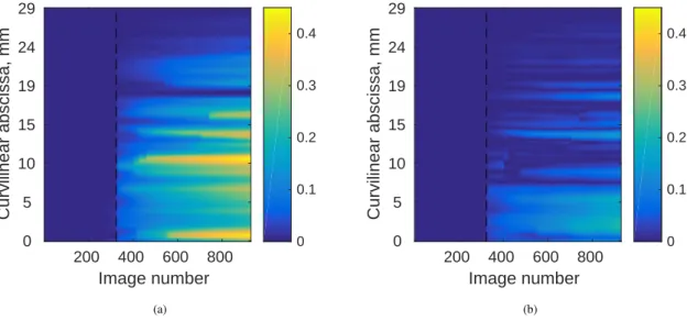
Figure 10 shows the space-time maps of the crack opening displacement (COD) that was obtained by computing the displace-ment jump for each split node for which its curvilinear abscissa was calculated along the crack path. The COD uncertainty was evaluated for the first 324 pictures for which the RMS residuals were virtually identical for both meshes (Figure 8(b)). Conse-quently, it was assumed that no crack had initiated. The standard COD uncertainty was equal to 0.03 pixel (or about 2 µm). This level is twice that observed on average for all the nodes (Table 4). A COD being obtained as the difference of two displace-ments, its variance is twice that of the nodal displacements (since it is uncorrelated). Further, the variance of edge nodes is on

200 400 600 800 Image number 0 5 10 15 19 24 29 Curvilinear abscissa, mm 0 0.1 0.2 0.3 0.4 (a) 200 400 600 800 Image number 0 5 10 15 19 24 29 Curvilinear abscissa, mm 0 0.1 0.2 0.3 0.4 (b)

FIGURE 10Mode I (a) and II (b) COD profiles as functions of time, expressed in mm, for each point along the crack path. For

the mode II, the absolute value is considered and the same dynamic range is used in both sub-figures. The dashed line depicts the regimes prior to and after crack initiation (i.e., at image #324)

average twice that of bulk nodes [24]. Therefore, it is expected that the standard COD uncertainty is two times that of nodal displacements, which is exactly what was observed. Given the fact that the COD amplitudes reached up to 6 pixels, such levels were deemed trustworthy since they were two orders of magnitude greater than the measurement uncertainties.

The mode I (i.e., opening) component was generally higher than the absolute mode II (i.e., in-plane shear) contributions, except close to the notch root, which indicated that crack initiation occurred under mixed mode condition. This observation may explain why the crack did not initiate parallel to the notch direction but at an angle of about 45° (Figure 5). The notch root geometry associated with material heterogeneities (e.g., air bubbles, aggregates in the millimeter range) and superficial drying cracks of the cementitious matrix (although minimized by sample conservation at 100% relative humidity) may promote off-axis crack initiations (as observed in other samples). Last, special caution has to be exercised since these analyses only rely on one lateral surface and may depend on the underlying microstructure.

The DIC measurements using the first mesh (Figure 3) were further post-processed to evaluate the notch opening displacement (NOD). Two zones of interest (ZOIs) were selected, and the NOD was then determined as the difference of average displacements over both ZOIs (Figure 11). In the present case, there is one instance for which crack propagation is very fast, namely, when the

0 100 200 300 400 0 200 400 600 800 1000 1200

Force, N

image number

FIGURE 11(a) Load vs. notch opening displacement (NOD) measured via DIC and comparison with the clip gauge data (for

the same temporal discretization as image acquisition). The two ZOIs over which the displacements are averaged are shown as red boxes in the inset. (b) Difference between NOD measurements using the clip gauge and DIC vs. image number. The dashed line depicts the regimes prior to and after crack initiation (i.e., at image #324)

NOD varies between 35 and 59 µm in 0.67 s and the load decreases from 765 to 444 N. It is worth mentioning that even though the NOD measurements of the clip gauge and DIC were not performed exactly at the same location (see inset of Figure 11(a)), the results are very consistent with an RMS difference of 11.7 µm (i.e., 0.16 pixel) for the full curve, but considerably smaller if only the first 324 images are considered, namely, 2.2 µm (i.e., 0.03 pixel, which is of the order of the measurement uncertainty).

This difference may be due to the fact that when the crack propagates, 3D effects are more important, and the two responses no longer coincide exactly. It is worth noting that thanks to DIC, it may be possible to fully suppress the need for clip gauges, not only reducing costs but also obtaining more information of the test to feed simulations and identification procedures, as proposed in this paper.

One additional advantage of using DIC for the NOD measurement in comparison to the clip gauge is the direct access to the mode II NOD [27]. Both mode I and II components are shown in Figure 12. Even though the crack initiates at a 45° angle and propagates along a complex path, the NOD profiles show that the studied experiment is close to a pure mode I test at the macroscopic level (e.g., the maximum amplitude of mode I NOD is equal to 330 µm in comparison to 20 µm for the mode II component). Another interesting point is the NOD jump from image #324 to #325 of 23 µm for mode I and less than 3 µm for mode II. 0 250 500 750 1000

image number

FIGURE 12Histories of mode I (opening) and II (in-plane shear) NODs

Last, an estimate of the fracture energy can be obtained as the integral of the load vs. NOD curve divided by the nominal cracked surface, namely, 𝐽𝑐 ≈ 66J/m2_{, which is very close to the estimate obtained with the clip gauge (Table 2). These new}

results additionally validate the DIC analysis in the presence of a major crack.

3

NUMERICAL PROCEDURES

The following section summarizes the numerical procedures applied herein. First, the geometry, boundary conditions, and constitutive models for the FE simulations are described. Then, the identification procedure is briefly discussed.

3.1

Finite Element Model

The finite element (FE) code Abaqus™ [1] was run for the analyses reported herein. The mesh used in the FE model was based on that used in DIC analyses (Figure 7). The cohesive elements were introduced along the curved crack path as explained in Section 2.2 (Figure 6(b)). For the elastic part, three-node plane strain elements (CPE3) were used with homogeneous properties over the whole sample. The plane strain hypothesis is made because of the large width (i.e., 38.5 mm) to height (i.e., 40 mm) ratio. The so-called PPR model was selected [36, 35]. It is considered that CZM parameters for mode I and mode II are the same since the sensitivity for mode II is very low in the present case. The parameters of the PPR model that defines the curve,

i.e., the shape parameters (𝛼 and 𝛽) and the initial slope (𝜆𝑛 and 𝜆𝑡) were chosen equal to 7 and 0.005 respectively [51]. To

illustrate the selected CZM, Figure 13 shows the traction-separation law using the PPR model with the initial parameters. The initial slope was selected to be steep enough to make sure that spurious elastic softening was mitigated, but not too much for numerical purposes. With the selected shape parameters, the softening response at the end (i.e., beyond 20 µm separations) can help better describe fracture phenomena in concrete-like materials [15]. For the converged properties, it was checked that considering 𝛼 = 2 (i.e., linear decay) did not significantly change the results reported hereafter (in terms of residual levels) as it essentially alters the cohesive strength 𝜎𝑚𝑎𝑥. The overall shape of the traction-separation law shown in Figure 13 will be identical for all the following analyses.

FIGURE 13Mode I traction-separation law with the initial parameters considered herein

Since the displacement levels were small (i.e., in the sub-pixel range for most of the analysis) and there was not much contrast in the images, they were too noisy when directly prescribed as boundary conditions. Therefore, the nodal displacements measured by DIC were temporally filtered with a moving average using 25 points and then utilized as Dirichlet boundary conditions at the

nodes highlighted in red circles in Figure 7. It is worth noting that even using this temporal regularization, it will be shown that there still are fluctuations due to measurement uncertainties in the following analyses. The displacement field measured for the very first image was taken out from the subsequent time steps to avoid the consideration of the preloading of the sample, and similarly for the measured load.

3.2

Identification Procedure

The identification was carried out using the Finite Element Model Updating (FEMU [34]) scheme. The cost function was written to minimize the gap between the experimental applied load and the calculated force. Let us consider the instantaneous force residual

𝑅_𝐹(𝑡, {𝐩}) = 𝐹exp(𝑡) − 𝐹FE(𝑡, {𝐩}) (3) where 𝐹exp_{is the experimental force (i.e., measured by the load cell), 𝐹}FE _{the vertical force calculated in the FE simulations}

for the top Dirichlet node (Figure 7), and {𝐩} the column vector with the chosen parameters. The identification was performed with a nonlinear least squares minimization scheme of 𝜒2

𝐹 𝜒_𝐹2({𝐩}) = 1 𝑛_𝑡𝛾2 𝐹 ∑ 𝑡 𝑅2_𝐹(𝑡, {𝐩}) (4)

and thus this procedure will be referred to as FEMU-F hereafter. 𝑛𝑡denotes the number of time steps, and 𝛾𝐹 the standard load uncertainty. The minimization of Equation (4) was performed via a Gauss-Newton scheme. The latter consists in approximating, at iteration 𝑛, about the current estimate {𝐩𝐧}of the parameters

𝐹FE(𝑡, {𝐩𝐧} + {𝛅𝐩}) ≈ 𝐹FE(𝑡, {𝐩𝐧}) + 𝜕𝐹FE

𝜕{𝐩}(𝑡, {𝐩𝐧}){𝛅𝐩} (5) and coupling Equations (3) and (4) in order to minimize the load residuals with respect to {𝛿𝐩}, thereby leading to linear systems in terms of parameter corrections {𝛿𝐩}

[𝐇]{𝛿𝐩} = {𝐡} (6)

where [𝐇] is the Hessian matrix, and {𝐡} the Jacobian vector. For these quantities, the load sensitivities 𝐒𝐅to each considered

parameter of 𝐹FE_{were calculated [47]. Herein, it was chosen to use finite differences with a 1% perturbation of each individual}

parameter. At each time step 𝑡, a line vector was obtained {𝐒𝐅(𝑡, {𝐩})} =

𝜕𝐹FE

𝜕{𝐩}(𝑡, {𝐩}) (7)

so that the Hessian [𝐇] reads

and the Jacobian {𝐡}

{𝐡} = [𝐒𝐅({𝐩})]⊤{𝐑𝐅({𝐩})} (9)

where [𝐒𝐅({𝐩})]denotes the sensitivity matrix that concatenates all line vectors {𝐒𝐅(𝑡, {𝐩})} over time, and {𝐑𝐅({𝐩})} all

instantaneous equilibrium residuals 𝑅𝐹(𝑡, {𝐩}).

The FEMU-F procedure was implemented within the Correli 3.0 framework [31] in which Abaqus™ is called whenever needed for updating a current solution or computing the load sensitivities. The convergence criterion was set for the RMS of the parameter updates reaching less than 1% their current level.

4

RESULTS

This section gathers the results of all the numerical analyses. First, uncertainty and sensitivity analyses are carried out to check whether the sought parameters are identifiable, and if so, at which time steps of the experiment. Further, the identification procedure uses different steps to avoid as much as possible local minima. Last, the results are validated with pieces of information of the experiment that were not used in the calibration, namely, displacement fields and registration residuals.

4.1

Load uncertainty due to Dirichlet boundary conditions

It is proposed to calibrate the CZM parameters using only the loading curve of the test via a FEMU-F procedure. The load uncertainty is important to check whether the parameters can be calibrated. Although the load cell had a nominal standard uncertainty of about 2.5 N, it is proposed to evaluate the contribution of the DIC displacement uncertainties on the reaction forces when they are applied as Dirichlet boundary conditions on the FE model (Figure 7).

A first simulation is run with the proposed model, for the first 100 time steps to ensure that no crack propagation occurred. It is worth noting that the Young’s modulus calibrated in Section 4.3.1 is used instead of its initial level in the identification procedure. Then, for each time step, each of the six applied displacements (i.e., horizontal and vertical components for each of the three nodes highlighted in Figure 7) was perturbed with a random centered Gaussian noise with a standard deviation equal to the standard displacement uncertainty (i.e., 0.015 pixel or 1.1 µm, which was subsequently filtered with a moving average using 25 temporal data as performed with the experimental measurements). The standard deviation of the reaction force difference of the top node (Figure 7) for all time steps of these two analyses is calculated to estimate the load uncertainty. The procedure is then repeated 100 times and resulted in an average standard deviation of 40 N, namely, about sixteen times higher than the load cell uncertainty. It is worth noting that if the temporal filtering is not accounted here, this estimate reached 110 N, which points toward the need for temporal filtering. All these analyses show that, in the present case, displacement uncertainties in the micrometer range (or possibly below) are required to get good estimates of elastic parameters.

As will be shown hereafter, this is a major source of limitation. For the sake of comparison, a standard load uncertainty

𝛾𝐹 = 40N will be considered in all subsequent analyses.

4.2

Sensitivity Analysis

Before performing the calibration itself, sensitivity analyses are very useful to make sure that all the parameters of the selected model are identifiable [18, 3, 51]. In the present case, the load sensitivities were computed for parameter offsets 𝜖 = 1%. The considered parameters were the ones gathered in Table 2 (Poisson’s ratio excluded) that were used to start the calibration procedure.

Figure 14 reports the sensitivities of the three selected parameters. The Young’s modulus is the most sensitive parameter,

0 50 100 150 200 250 300 350 0 500 1000 1500 2000 S F , N/ E max J c

FIGURE 14Load sensitivities to the three considered parameters for 𝜖 = 1% variation. The first dashed line depicts the

pre-peak part (i.e., elastic regime prior to image #287), the second defines the first step of crack initiation (i.e., at image #325), and the third delimits the series of images used in the first step of the CZM calibration (i.e., image #350)

which indicates that the behavior of mortar, as expected, remains essentially elastic throughout the whole test. For a 1% offset, the load variations are very high for the elastic parameter (i.e., more than two orders of magnitude higher than 𝛾𝐹), and with a maximum about ten times higher than 𝛾𝐹 for the cohesive parameters. The sensitivity to the cohesive strength 𝜎max, which is

significant, occurs over a limited time duration that corresponds to the crack initiation regime. Similarly, the fracture energy 𝐽𝑐, which controls crack propagation, leads to sensitivities that mostly cancel out during the second part of the experiment. It is interesting to note that the rise of the curves related to the cohesive strength and fracture energy are related to the sudden drop of the one related to the Young’s modulus, when part of the elastic energy stored in the sample is converted into new crack surfaces.

The decimal logarithm of the associated absolute Hessian is shown in Figure 15(a). When diagonalized (Figure 15(b)), it was concluded that the condition number was of the order of 200, and all eigen values were very large in comparison to zero. Consequently, all three parameters can be determined with the present data at hand. Figure 15(c) shows that the first eigen vector is dominated by the Young’s modulus, as was expected from the analysis of the load sensitivities. The second eigen vector is mostly dependent on the fracture energy, and the third one on the cohesive strength. The latter leads to the lowest eigen vector, namely, it will be the most difficult to calibrate.

6.5 7 7.5 8 8.5 (a) 6 6.5 7 7.5 8 8.5 9 (b) -1 -0.5 0 0.5 1 (c)

FIGURE 15 (a) Decimal logarithm of the absolute Hessian [𝐇] (expressed in (N/𝜖)2) for 𝜖 = 1% variation. (b) Decimal

logarithm of diagonalized Hessian (expressed in (N/𝜖)2_{), and (c) corresponding eigen vectors}

4.3

Parameter Calibration

In this section, the identification consists of calibrating one parameter related to the elastic behavior (i.e., Young’s modulus

𝐸) and two for the CZM (i.e., cohesive strength 𝜎_maxand fracture energy 𝐽𝑐). As shown in Figure 14, both CZM parameters

induced no sensitivity in the initial loading steps (since no crack had initiated yet). For the numerical approach, it is important to initialize the identification with reasonable values for avoiding local minima or divergence [47].

Three steps were considered in the identification procedure. First, the Young’s modulus was calibrated, and then both CZM parameters, using few time steps, and then the full curve. The initial parameters were based on the data gathered in Table 2. The Young’s modulus was directly the measured property, and the value for the cohesive strength was assumed to be equal to the ultimate tensile strength. The fracture energy was selected higher than its estimate obtained with the load vs. NOD curve (Section 2.2), as will be explained in Section 4.3.2.

4.3.1

Elastic parameter

The load sensitivity to the Young’s modulus is shown in Figure 16(a) for the experimental pre-peak load levels (i.e., first 295 time steps). The algorithm was initialized with 𝐸 = 29 GPa and converged to 𝐸 = 13.4 GPa in only two iterations due to its

linearity with respect to the applied load (Figure 16(b)). From an initial RMS force residual of 593 N, it decreased to 92 N after convergence, which is about twice the estimated load uncertainty 𝛾𝐹. It is worth noting that in the present case, the load fluctuations are higher in the FE simulation than in the experiment since experimentally measured displacements (which are noisy) were applied as boundary conditions.

-10 0 10 20 -200 0 200 400 600 800 1000 S F , N/ Young's modulus (a) -10 0 10 20 0 500 1000 1500 2000 Force, N experimental initial converged (b)

FIGURE 16(a) Load sensitivity to the Young’s modulus for 𝜖 = 1% variation. (b) Initial and final load histories for the pre-peak

images, and comparison with the experimentally measured data

The Young’s modulus decreased significantly between its initial guess and the converged solution. One reason may be related to the fact that only one surface was analyzed herein. Had the two opposite surfaces been monitored via DIC, different levels may have possibly be observed since the experimental boundary conditions would have been better captured [10]. This point highlights that measurements of Young’s modulus using only data from one side of the specimen may lead to very different results.

4.3.2

CZM parameters

Once the Young’s modulus was calibrated, the CZM parameters were determined. It was chosen not to let the former change. For this case, only the first 350 images were considered since the crack was already well formed (see gray level residuals shown in Figure 17 for the first DIC mesh, for image #350) even though its opening was still small (Figure 10). For the chosen images, the crack has not yet fully propagated and thus less artifacts related to the microstructure and out of plane propagation interfere with the results. Further, the sensitivity analysis (see Figure 14) shows that the sought cohesive parameters are the most sensitive for this first part of the test. Last, since less images are considered, the FE simulations run faster. The converged solution can also be used as initialization of longer analyses that generally induce less iterations.

-30 -20 -10 0 10 20

FIGURE 17Gray level residual field for the DIC analysis of the 350-th image using the mesh of Figure 3

The sensitivities to both parameters are shown in Figure 18(a), from image #295 on (i.e., starting from the last one used in the calibration of the elastic parameter). In the FEMU-F analysis, since the dependence to the parameters were nonlinear, the updates per iteration were limited (i.e., 5% in the present case) to avoid very sever fluctuations at the beginning of the optimization process. In the present case, the initial cohesive strength 𝜎max= 5.8MPa was considered (i.e., identical to the net

flexural strength). However, the initial fracture energy was set to 𝐽𝑐 = 100J/m2, i.e., about 1.5 times the estimate from the load vs. NOD curve (Table 2). The higher initial fracture energy was used to avoid negative eigenvalue errors in Abaqus™ for the

20 40 60 80 -500 0 500 1000 1500 S F , N/ Cohesive strength Fracture energy (a) 0 20 40 60 80 0 200 400 600 800 1000 Force, N experimental initial converged (b)

FIGURE 18(a) Load sensitivities to the cohesive strength and fracture energy of the CZM for 𝜖 = 1% variation for the initial

iteration. (b) Initial and final load histories for the analyzed images, and comparison with the experimentally measured data

iterations when the crack started to propagate when initialized with 𝐽𝑐= 68J/m2_{. The code converged after 7 iterations, and the}

are slightly different from image #320 on, and that the converged state better captures the sudden crack propagation (i.e., sudden drop of force) at image #324. The RMS force residual decreased from 93 N to 87 N, which again is close to twice the load uncertainty. Consequently, the identification quality associated with the Young’s modulus, and cohesive parameters is identical. The calibrated parameters are gathered in Table 5. It is worth noting that the fracture energy is 20% higher than the estimate obtained from the load vs. NOD curve. If 10 images are added in this calibration, the cohesive strength 𝜎max converges to

4.7 MPa, while 𝐽𝑐remains closer to the last estimate, converging to 74 J/m2_{. Conversely, the cohesive strength is less stable in}

the calibration in comparison to the ultimate tensile strength, as expected from the sensitivity analysis.

TABLE 5Calibrated parameters via FEMU-F

Young’s modulus (𝐸) 13.4 GPa Cohesive strength (𝜎𝑚𝑎𝑥) 6.2 MPa Fracture energy (𝐽𝑐) 79 J/m2

The characteristic fracture length [25]

𝓁𝐻 =

𝐸𝐽_𝑐 𝜎2

max

(10) is of the order of 2.8 cm when the calibrated parameters are used (Table 5), or 4.5 cm, if 𝜎max= 4.7MPa and 𝐽𝑐 = 74J/m2are

considered. The fracture process zone size, which is a fraction of it [44], amounts to few millimeters, which is very small. This observation also explains why the sensitivities to 𝜎maxand 𝐽𝑐 are rather low for the second part of the experiment (Figure 14),

and that no secondary crack was detected.

4.3.3

Full curve

Last, the identification is performed using all time steps, and the parameters reported in Table 5. Since the initialization is taken with pre-calibrated parameters, their change was set to a maximum of 10% per iteration. It converged after 10 iterations, reducing the RMS force residuals from 182 N to 164 N (i.e., about 4 times the standard load uncertainty). The final loading curves are shown in Figure 19.

0 50 100 150 200 250 300 350 -200 0 200 400 600 800 1000 Force, N experimental initial converged

FIGURE 19Initial and final full load histories for the analyzed images, and comparison with the experimentally measured data

Although the initial curve shows a better fit right after the peak, the converged state improves especially after the time step #350, which was not included in the previous identification step. However, the overall identification quality has degraded by a factor of two in comparison with the previous result that focused on the first 350 images. This result indicates that the cohesive model does not fully account for the final stages of crack propagation. The converged parameters of this analysis are gathered in Table 6. The calibration of the CZM parameters using the full curve was more stable than in the previous step, since the parameter sensitivities were higher. However, initializing with 𝜎max= 4.7MPa or 𝜎max= 6.2MPa, FEMU-F converged to the

same final parameters. The fact the two sets of parameters led to the order of magnitude of load residuals (i.e., about 4 times the standard load uncertainty) is that the model error is similar in both cases. Considering this last set of parameters (Table 6) in Equation (10), the characteristic fracture length now becomes 𝓁𝐻 = 5.9cm, which is twice higher than for the previous estimate, but still leading to millimetric fracture process zone sizes.

TABLE 6Calibrated parameters via FEMU-F in the full curve

Cohesive strength (𝜎𝑚𝑎𝑥) 5.9 MPa Fracture energy (𝐽𝑐) 152 J/m2

4.4

Validation

A large part of the information that could be extracted from the test was not used in the identification procedure, i.e., displacement fields and gray level residuals. Thus they can be used to validate the calibration results. The nodal displacement difference between FE simulations using the last set of parameters (Table 6) and DIC analyses, which are gathered in the column vector

{𝛿𝛖}, are calculated. The corresponding RMS displacement residuals RMS({𝛿𝛖}) = √ 1 𝑛_dof ∑ 𝑑𝑜𝑓 ( 𝜐DIC_𝑖 − 𝜐FE_𝑖 )2 (11)

where 𝑛dofis the number of degrees of freedom, 𝜐DIC𝑖 nodal displacements of DIC analyses, and 𝜐FE𝑖 nodal displacements of FE simulations are shown in Figure 20. The RMS residual is on average equal to 0.15 pixel for the first set of images (i.e., about 10 times the standard displacement uncertainty), and increases to 0.39 pixel (i.e., about 26 times the standard displacement uncertainty) from image #325 until the last one. From these results, it is also concluded that a higher model error occurs in the second part of the experiment (even though there is already a model error in the first part), namely, the selected CZM and the numerical model are not able to fully capture the complexity of the cracking mechanism.

0 250 500 750 1000 Image number 0 0.1 0.2 0.3 0.4 0.5 RMS displacement residual, px

FIGURE 20 RMS displacement residuals between FE simulation and DIC analysis as functions of the image number. The

dashed line depicts the regimes prior to and after crack initiation (i.e., at image #324)

The gray level residuals are directly computed from the images, by using the resulting displacement fields from the FE analysis (i.e., 𝜌FE_{(𝐱) = 𝑓 (𝐱) − 𝑔(𝐱 + 𝐮}FE_{(𝐱))). This is possible because the FE simulations were driven by measured boundary conditions.}

The results are shown in Figure 21. Although an offset is seen, the mean difference is 0.45 gray level, smaller than 0.2% of the dynamic range of the 8-bits image. The mean RMS difference is equal to 0.40 gray level when calculated until image #324 (represented by the dashed line in Figure 21), and 0.48 gray level from image #325 to the end of the test. The global degradation is an additional indication that the numerical simulation is not fully capturing the crack propagation process.

0 250 500 750 1000 Image number 1.2 1.4 1.6 1.8 2 2.2 2.4 2.6 RMS residual, GL FEM DIC (a) 0 250 500 750 1000 Image number 0.1 0.2 0.3 0.4 0.5 0.6 0.7 0.8 RMS residual, GL (b)

FIGURE 21(a) RMS gray level residuals as functions of the image number for the FE simulation and the DIC analysis and

(b) the difference between both curves. The dashed line depicts the regimes prior to and after crack initiation (i.e., at image #324) One additional analysis is proposed, since the CZM parameters were calibrated in two steps. The residuals in displacement and in gray level between these two analyses are summarized in Figure 22. Figure 22(a) reports the difference between the RMS displacement residuals with respect to DIC measurements. It is shown that from image #325 to the end of the test, the RMS difference is on average equal to 0.015 pixel (i.e., identical to the DIC displacement uncertainty), with the highest value being close to the onset of propagation.

0 250 500 750 1000 Image number -0.01 0 0.01 0.02 0.03 0.04 0.05 Difference in Ures, px (a) 0 250 500 750 1000 Image number -0.05 0 0.05 0.1 0.15 0.2 Difference in GLres, GL (b)

FIGURE 22Residual differences for CZM parameters of Sections 4.3.3 with respect to those of Section 4.3.2 in terms of (a)

A similar trend is observed in Figure 22(b) for the gray level differences. Although using 𝜎max= 5.9MPa and 𝐽𝑐 = 152J/m2

(Table 6) led to slightly lower force residuals, higher residuals in terms of displacements and gray levels are observed in com-parison to using 𝜎max= 6.2MPa and 𝐽𝑐 = 79J/m2(Table 5). This observation shows that the first set of parameters should not

be discarded, and is at least as good as the second one to describe the experiment analyzed herein.

It is noteworthy how the identified fracture properties were close to those obtained for the material with experiments, especially when approaching a noisy data set, and identifying a very different Young’s modulus. Considering that most of the effects of the out of plane crack propagation are gathered in the energy parameter, it may be argued that to estimate the fracture energy in such cases, it is better not to use the full set of data, and only until the crack is well defined but has not fully propagated. For the cohesive strength, a higher uncertainty (related to smaller sensitivity, see Figure 18(a)) is seen, and although more uncertain, it may give a first estimation for more complex models and avoid the need for other experiments.

4.5

Geometrical validation

One may wonder whether the effort to describe a curved crack was necessary. To answer that question, one last study was performed. A mesh with a straight crack (see Figure 23) was used to check whether the properties obtained by the identification with the curved crack would be reasonable for this case. The same GMSH procedure was followed but the crack was assumed to be vertically straight and centered about the notch root. The mesh density is approximately the same as before with the same number of cohesive elements (i.e., the vertical coordinates of the new cohesive nodes are identical to the previous case).

FIGURE 23Mesh used to check the influence of a straight crack path on the predictive power of the CZM

By analyzing the whole test with the properties identified in Section 4.3.3, the RMS load residual is equal to 145 N, which is lower than the level reported for the curved crack (i.e., 164 N), as shown in Figure 24. Most of the improvement is for the early stages of crack propagation (i.e., NOD < 50µm), but it is very similar otherwise. If the calibration is performed using

this set of parameters as initial guess, it converges after 5 iterations to an RMS load residual of 119 N, when 𝜎𝑚𝑎𝑥= 6.7MPa and 𝐽𝑐 = 170J/m2_{. These levels are higher than those observed for the curved crack (Table 6). The cohesive strength is very}

close to the tensile strength determined from Brazilian tests (Table 2). The crack length being smaller for the straight crack, it is compensated by a higher fracture energy in comparison to the curved crack. A first order estimate of the work of fracture is given by 𝑊𝑐 = 𝐽𝑐𝓁𝑐𝑤, where 𝓁𝑐is the crack propagation length (for the damaged elements) and 𝑤 the width of the sample (i.e., under the hypothesis that the crack propagates equally through the width). For the straight crack, 𝑊𝑐 is equal to 169 mJ, and 167 mJ for the curved crack. The fact that these two values are close shows that the identified fracture energies lead to the same work of fracture (or macroscopic dissipation) for curved or straight cracks. The levels are significantly larger than the evaluation based on the measured force vs. NOD curve shown in Figure 2 (i.e., 𝑊𝑐 = 74mJ). These differences are mostly concentrated on the second regime of propagation (when NOD > 50 µm, Figure 24), where a significantly lower amount of energy is dissipated in the experiment but a lot more in the simulations (possibly due to imperfect boundary conditions).

0 50 100 150 200 250 300 350 0 200 400 600 800 1000 Force, N experimental straight crack curved crack

FIGURE 24 Full load histories for the analyzed images with curved and straight cracks compared with the experimentally

With no additional information, it would be concluded that the details of the crack geometry are not important. However, there are other sources of information, namely those provided by displacement fields and gray level residual maps. The RMS displacement residuals are shown in Figure 25. The result for the curved crack is the same as that of Figure 20. Even before image # 324, the RMS residuals are significantly higher (i.e., about two to three times) for the straight crack than for the curved crack. For the second part of the test, during crack propagation, the difference increases even more (i.e., up to four times). In terms of kinematic data, there is very clear degradation of the prediction quality for the simplified geometry.

0 250 500 750 1000 Image number 0 0.5 1 1.5 2 2.5 RMS displacement residual, px straight crack curved crack

FIGURE 25RMS displacement residuals between FE simulations considering curved or straight cracks. The dashed line depicts

the regimes prior to and after crack initiation (i.e., at image #324)

From the simulated kinematic fields, the gray level residuals can be computed for the same reasons as those discussed above. They are shown in Figure 26. Before image #324, small differences are seen (i.e., they are slightly higher for a straight crack), but more discrepancies thereafter. Since the crack path is not well described, the residuals increase a lot more once that the crack is more developed. At the end of the test, while the curved crack led to residuals about 50% higher than DIC, the straight crack induced levels up to 200% higher.

0 250 500 750 1000 Image number 1 1.5 2 2.5 3 3.5 RMS residual, GL straight crack curved crack DIC (a) 0 250 500 750 1000 Image number 0 0.2 0.4 0.6 0.8 1 1.2 1.4 RMS residual, GL straight crack curved crack (b)

FIGURE 26(a) RMS gray level residuals as functions of the image number for the FE simulations, with the curved and straight

crack meshes, and the DIC analysis (using the adapted mesh) and (b) the difference between both curves to DIC. The dashed line depicts the regimes prior to and after crack initiation (i.e., at image #324)

If only a straight crack were considered, one could mistakenly conclude that by having low force residuals, and the properties would be well identified. This is the case if only global (i.e., at the macroscopic scale) load data are used. When kinematic fields are then used for validation purposes, the geometric details of the crack path at the mesoscopic scale have a more significant influence. These results emphasize the importance of validating the calibrated models against independent data at various scales (i.e., here the displacement fields at the mesoscale and gray level residual maps at the microscale).

5

SUMMARY AND PERSPECTIVES

A numerical approach to identify the parameters of a cohesive zone model of a curved crack was presented. Starting from digital image correlation analyses, the gray level residuals were used to construct a suitable mesh for finite element simulations and model updating of a curved crack. It is worth noting that no artificial pattern was applied to the monitored surface.

The uncertainty related to using noisy displacements as Dirichlet boundary conditions was assessed, and the sensitivities to each parameter provided an insight into their identifiability. Displacement fields and gray level residuals allowed the calibration to be validated since only the load measurements of the tests were used in the calibration scheme in addition to displacements of three points.

When the calibration was performed on the first propagation stage only, the level of the cohesive strength was similar to that of the tensile strength of the material obtained from flexural and Brazilian tests. Similarly, the cohesive energy had the same order of magnitude as the fracture energy evaluated from the load vs. notch opening displacement curve. This first regime of

propagation was very well captured by the selected model. Conversely, when the full propagation stage was considered, higher fracture energies were estimated with a higher model error, thereby signaling more deviations with respect to the experiment. It is worth noting that the RMS load residuals varied between 2 and 4 times the uncertainties associated with the fact that measured boundary conditions were prescribed to FE simulations. Given the complexity of the present situation, such levels are remarkably low and show that the CZM considered herein can be used to model cracking of the studied mortar especially at the early stages of propagation.

The validity of CZM was studied for the actual crack path and a straight crack. If the predictive capacity was only probed at the macroscale with the load residuals, there was no significant gain in accounting for the geometric details of the propagation path. In the present case, lower RMS residuals were observed for the straight path. Conversely, when displacement fields and gray level maps were compared at more local (i.e., mesoscopic and microscopic) scales, the actual geometry led to significantly better results.

It is worth noting that the analyses presented herein relied on monitoring a single face of a rather thick beam. As such, it only partially captured the complexity of the crack surface, prevented a satisfactory calibration of the Young’s modulus, and a full validation of the CZM. By monitoring opposite faces of the sample, more data would be available for more complete analyses of the test via 2D [49, 50, 51] or 3D analyses. Further, in situ tests and measurements via digital volume correlation may enable for the estimation of 3D cracked surfaces and crack fronts [38, 23]. Last, no material heterogeneities were accounted for and only macroscopic (and deterministic) properties were calibrated. Full 4D analyses (3D + time) [8] would be required to fully characterize more local properties, and repeated tests would be required to evaluate their scatter.

Although it was shown that a difficult case for DIC could be used, after this analysis it is believed that the uncertainty of the identification could be reduced mainly along three directions, namely, applying a speckle pattern on the sample surface for achieving higher contrasts, controlling the test with the clip gauge measurement instead of stroke to reduce the likelihood of crack jump between small time steps (e.g., due to snap-back responses), by monitoring opposite faces of the test (e.g., for a better calibration of the Young’s modulus, and possibly by using other CZMs).

Similar approaches as those discussed herein are of special interest when an increasing R-curve behavior is expected and can be applied to many other brittle materials. For further studies, tackling different experimental setups (e.g., 4-point flexural or wedge splitting tests), different materials, or analyzing more samples to check the consistency, would be straightforward follow-ups. Combining more kinematic data than used herein for calibration purposes (or directly the pictures in integrated frameworks [29, 31, 22, 9]) was considered to be out of this paper scope. Last, crack branches, coupling opposite face analyses, and 3D models could give further insight into crack propagation and its interaction with the material microstructure.

ACKNOWLEDGMENTS

This work was performed within the FAPESP-CNRS SPRINT project, grant #2018/15266-0, São Paulo Research Foundation (FAPESP). The experimental work reported herein was carried out within the framework of the CEA-EDF-Framatome agree-ment. This study was also partially supported by the Coordenação de Aperfeiçoamento de Pessoal de Nível Superior - Brasil (CAPES) - Finance Code 001. The PhD project of RV is supported through grant #2018/23081-0, São Paulo Research Foundation (FAPESP).

References

[1] 2014: Abaqus 6.14 Documentation. Dassault Systèmes Simulia Corp., Providence, RI, USA.

[2] AFNOR, 2012: Essais pour béton durci - Partie 6 : détermination de la résistance en traction par fendage d’éprouvettes. Standard NF EN 12390-6, AFNOR, Paris (France).

[3] Alfano, M., G. Lubineau, and G. H. Paulino, 2015: Global sensitivity analysis in the identification of cohesive models using full-field kinematic data. International Journal of Solids and Structures, 55, 66–78.

[4] Aure, T. and A. Ioannides, 2010: Simulation of crack propagation in concrete beams with cohesive elements in abaqus.

Transportation Research Record: Journal of the Transportation Research Board, no. 2154, 12–21.

[5] Barenblatt, G., 1962: The mathematical theory of equilibrium of crack in brittle fracture. Adv. Appl. Mech., 7, 55–129. [6] Bažant, Z. and X. Yunping, 1994: Drying creep of concrete: constitutive model and new experiments separating its

mechanisms. Materials and Structures, 27, no. 1, 3–14.

[7] Besnard, G., F. Hild, and S. Roux, 2006: “Finite-Element” displacement fields analysis from digital images: Application to Portevin-Le Chatelier bands. Experimental Mechanics, 46, no. 6, 789–803.

[8] Buljac, A., C. Jailin, A. Mendoza, J. Neggers, T. Taillandier-Thomas, A. Bouterf, B. Smaniotto, F. Hild, and S. Roux, 2018: Digital Volume Correlation: Review of Progress and Challenges. Experimental Mechanics, 58, no. 5, 661–708.

[9] Buljac, A., V.-M. Trejo-Navas, M. Shakoor, A. Bouterf, J. Neggers, M. Bernacki, P.-O. Bouchard, T. Morgeneyer, and F. Hild, 2018: On the calibration of elastoplastic parameters at the microscale via X-ray microtomography and digital volume correlation for the simulation of ductile damage. European Journal of Mechanics - A/Solids, 72, 287–297.

[10] Carpiuc-Prisacari, A., M. Poncelet, K. Kazymyrenko, F. Hild, and H. Leclerc, 2017: Comparison between experimental and numerical results of mixed-mode crack propagation in concrete: Influence of boundary conditions choice. Cement and

Concrete Research, 100, 329–340.

[11] Carpiuc-Prisacari, A., M. Poncelet, K. Kazymyrenko, H. Leclerc, and F. Hild, 2017: A complex mixed-mode crack prop-agation test performed with a 6-axis testing machine and full-field measurements propprop-agation. Engineering Fracture

Mechanics, 176, 1–22.

[12] Charpin, L., Y. Le Pape, E. Coustabeau, E. Toppani, G. Heinfling, C. Le Bellego, B. Masson, J. Montalvo, A. Courtois, J. Sanahuja, and N. Reviron, 2018: A 12year edf study of concrete creep under uniaxial and biaxial loading. Cement and

Concrete Research, 103, 140–159.

[13] Choi, S. and S. P. Shah, 1997: Measurement of deformations on concrete subjected to compression using image correlation.

Experimental Mechanics, 37, no. 3, 307–313.

[14] Claire, D., F. Hild, and S. Roux, 2004: A finite element formulation to identify damage fields: The equilibrium gap method.

Int. J. Num. Meth. Engng., 61, no. 2, 189–208.

[15] Elices, M., G. Guinea, J. Gómez, and J. Planas, 2002: The cohesive zone model: advantages, limitations and challenges.

Engineering Fracture Mechanics, 69, 137–163.

[16] Evangelista, F., J. R. Roesler, and S. P. Proença, 2013: Three-dimensional cohesive zone model for fracture of cementitious materials based on the thermodynamics of irreversible processes. Engineering Fracture Mechanics, 97, 261–280. [17] Fagerholt, E., T. Børvik, and O. S. Hopperstad, 2013: Measuring discontinuous displacement fields in cracked specimens

using digital image correlation with mesh adaptation and crack-path optimization. Optics Lasers Eng., 51, no. 3, 299–310. [18] Fedele, R., B. Raka, F. Hild, and S. Roux, 2009: Identification of adhesive properties in GLARE assemblies using digital

image correlation. Journal of the Mechanics and Physics of Solids, 57, no. 7, 1003–1016.

[19] Ferreira, M., W. Venturini, and F. Hild, 2011: On the analysis of notched concrete beams: From measurement with digital image correlation to identification with boundary element method of a cohesive model. Engineering Fracture Mechanics,

78, no. 1, 71 – 84.

[20] Galenne, E. and B. Masson, 2012: A new mock-up for evaluation of the mechanical and leaktightness behaviour of NPP containment building. Proceedings SSCS 2012.

[21] Geuzaine, C. and J.-F. Remacle, 2009: Gmsh: A 3D finite element mesh generator with built-in pre-and post-processing facilities. International Journal for Numerical Methods in Engineering, 79, no. 11, 1309–1331.