HAL Id: hal-01313895
https://hal.archives-ouvertes.fr/hal-01313895
Submitted on 23 Jan 2017
HAL is a multi-disciplinary open access
archive for the deposit and dissemination of
sci-entific research documents, whether they are
pub-lished or not. The documents may come from
teaching and research institutions in France or
abroad, or from public or private research centers.
L’archive ouverte pluridisciplinaire HAL, est
destinée au dépôt et à la diffusion de documents
scientifiques de niveau recherche, publiés ou non,
émanant des établissements d’enseignement et de
recherche français ou étrangers, des laboratoires
publics ou privés.
Distributed under a Creative Commons Attribution| 4.0 International License
On the Periods of Spatially Periodic Preimages in Linear
Bipermutive Cellular Automata
Luca Mariot, Alberto Leporati
To cite this version:
Luca Mariot, Alberto Leporati. On the Periods of Spatially Periodic Preimages in Linear
Bipermu-tive Cellular Automata. 21st Workshop on Cellular Automata and Discrete Complex Systems
(AU-TOMATA), Jun 2015, Turku, Finland. pp.181-195, �10.1007/978-3-662-47221-7_14�. �hal-01313895�
On the Periods of Spatially Periodic Preimages in Linear
Bipermutive Cellular Automata
Luca Mariot and Alberto Leporati
Dipartimento di Informatica, Sistemistica e Comunicazione, Università degli Studi Milano - Bicocca,
Viale Sarca 336/14, 20124 Milano, Italy
l.mariot@campus.unimib.it, alberto.leporati@unimib.it
Abstract. In this paper, we investigate the periods of preimages of spatially pe-riodic configurations in linear bipermutive cellular automata (LBCA). We first show that when the CA is only bipermutive and y is a spatially periodic con-figuration of period p, the periods of all preimages of y are multiples of p. We then present a connection between preimages of spatially periodic configurations of LBCA and concatenated linear recurring sequences, finding a characteristic polynomial for the latter which depends on the local rule and on the configura-tions. We finally devise a procedure to compute the period of a single preimage of a spatially periodic configuration y of a given LBCA, and characterise the pe-riods of all preimages of y when the corresponding characteristic polynomial is the product of two distinct irreducible polynomials.
Keywords: Linear bipermutive cellular automata, spatially periodic configurations, preimages, surjectivity, linear recurring sequences, linear feedback shift registers.
1
Introduction
It is known that if F : AZ→ AZis a surjective cellular automaton (CA) and y ∈ AZis a
spatially periodic configuration, then all preimages x ∈ F−1(y) are spatially periodic as well [2]. However, to our knowledge there are no works in the literature addressing the problem of actually finding the periods of such preimages.
The aim of this paper is to study the relation between the periods of spatially peri-odic configurations and the periods of their preimages in the case of linear bipermutive cellular automata(LBCA). Given a spatially periodic configuration y ∈ AZof period
p, we first prove that in generic bipermutive cellular automata (BCA) the period of a preimage x ∈ F−1(y) is a multiple of p, where the multiplier h ranges in {1, · · · , q2r}, with qbeing the size of the alphabet and r the radius of the BCA. We then show that, in the case of LBCA, a preimage x ∈ F−1(y) can be described as a concatenated linear recur-ring sequence(LRS) whose characteristic polynomial is the product of the characteristic polynomials respectively induced by the local rule f of the CA and by configuration y. Finally, we present a procedure which given a block x[0,2r−1]of a preimage x ∈ F−1(y)
determines the period of x, and we characterise the periods of all q2rpreimages of y when their characteristic polynomial is the product of two irreducible polynomials.
This research was inspired from the problem of determining the maximum number of players allowed in a BCA-based secret sharing scheme presented in [10].
The rest of this paper is organised as follows. Section 2 recalls some basic defini-tions and facts about cellular automata, linear recurring sequences and linear feedback shift registers. Section 3 shows that the periods of spatially periodic preimages are mul-tiples of the periods of their respective images, and characterises preimages of LBCA as concatenated linear recurring sequences. Section 4 focuses on the characteristic polyno-mial of concatenated LRS, while Section 5 presents an algorithm to compute the period of a single LBCA preimage and characterises the periods of all preimages of a spatially periodic configuration y in the particular case of irreducible characteristic polynomials. Finally, Section 6 summarises the results presented throughout the paper and points out some possible future developments on the subject.
2
Basic Definitions
2.1 Cellular Automata
Let A be a finite alphabet having q symbols, and let AZbe the full shift space consisting
of all biinfinite configurations over A. Given x ∈ AZ and i, j ∈ Z with i ≤ j, by x [i, j]
we denote the finite block (xi,··· , xj). In what follows, we focus our attention on
one-dimensional cellular automata, formally defined below:
Definition 1. A one-dimensional cellular automaton is a function F : AZ→ AZdefined
for all x ∈ AZand i ∈ Z as:
F(x)i= f (x[i−r,i+r]) ,
where f : A2r+1→ A is the local rule of the CA and r ∈ N is its radius.
From a dynamical point of view, a CA can be considered as a biinfinite array of cells where, at each time step t ∈ N, all cells i ∈ Z simultaneously change their state si∈ A by
applying the local rule f on the neighbourhood {i − r, · · · , i+ r}.
The main class of CA studied in this paper consists of bipermutive CA, defined as follows:
Definition 2. A CA F : AZ→ AZinduced by a local rule f : A2r+1→ A is called left
permutive (respectively, right permutive) if, for all z ∈ A2r, the restriction fR,z: A → A (respectively, fL,z: A → A) obtained by fixing the first (respectively, the last) 2r coordi-nates of f to the values specified in z is a permutation on A. A CA which is both left and right permutive is said to be abipermutive cellular automaton (BCA).
Another class of CA which can be defined by endowing the alphabet with a group structure is that of linear (or additive) cellular automata. We give the definition for the particular case in which A is a finite field. Thus, we have A= Fqwith q= ρα, where
ρ ∈ N is a prime number (called the characteristic of Fq) and α ∈ N.
Definition 3. A CA F : FZ
q→ FZq with local rule f: F2r+1q → Fqislinear if there exists
(c0,··· ,c2r) ∈ F2r+1q such that f can be defined for all(x0,··· , x2r) ∈ F2r+1q as:
f(x0,··· , x2r)= c0· x0+ ··· + c2r· x2r ,
One easily checks that if both c0and c2rin Definition 3 are nonzero then a linear CA is
bipermutive as well. Most of the results proved in this paper concern cellular automata which are both linear and bipermutive.
A configuration x ∈ AZ is called spatially periodic if there exists p ∈ N such that
xn+p= xnfor all n ∈ Z, and the least p for which this equation holds is called the period
of x. In this case, x is generated by the biinfinite concatenation of a string u ∈ Apwith itself, denoted by ωuω. A proof of the following result about preimages of spatially periodic configurations in surjective CA can be found in [2].
Lemma 1. Let F : AZ→ AZbe a surjective CA. Then, given a spatially periodic
con-figuration y ∈ AZ, each preimage x ∈ F−1(y) is also spatially periodic.
This lemma is a consequence of a theorem proved by Hedlund [7], which states that every configuration x ∈ AZ has a finite number of preimages under a surjective CA.
In the same work, Hedlund showed that bipermutive CA are also surjective. Indeed, given a BCA F : AZ→ AZinduced by a local rule f : A2r+1→ A and a configuration
y ∈ AZ, a preimage x ∈ F−1(y) is determined by first setting in x a block of 2r cells
x[i,i+2r−1]∈ A2r, with i ∈ Z. Then, denoting by fR,z−1: A → A and fL,z−1: A → A the inverses of the permutations obtained by respectively fixing the first and the last 2r coordinates of f to z ∈ A2r, for all n ≥ i+ 2r and n < i the value of xnis determined through the
following recurrence equation:
xn= fR,z(n)−1 (yn−r), where z(n)= x[n−2r,n−1], if n ≥ i + 2r (a) fL,z(n)−1 (yn+r), where z(n)= x[n+1,n+2r], if n < i (b) (1) As a consequence, by Lemma 1 the preimages of spatially periodic configurations under a BCA are spatially periodic as well. Moreover, since a preimage of y is uniquely deter-mined by a 2r-cell block using Equation (1), it follows that y has exactly q2rpossible preimages in F−1(y).
We now formally state the problem analysed in the remainder of this paper: Problem. Let y ∈ AZ be a spatially periodic configuration of period p ∈ N. Given a
BCA F : AZ→ AZ, find the relation between p and the spatial periods of the preimages
x ∈ F−1(y).
2.2 Linear Recurring Sequences and Linear Feedback Shift Registers
We now recall some basic definitions and results about the theory of linear recurring sequences and linear feedback shift registers, which will be useful to characterise the periods of preimages in LBCA. All the proofs of the theorems mentioned in this section may be found in the book by Lidl and Niederreiter [9].
Definition 4. Given k ∈ N and a, a0, a1, ··· , ak−1∈ Fq, alinear recurring sequence
(LRS) of order k is a sequence s= s0, s1,··· of elements in Fqwhich satisfies the
follow-ing relation:
The terms s0, s1, ··· , sk−1which uniquely determine the rest of the LRS are called the
initial valuesof the sequence. If a= 0 the sequence is called homogeneous, otherwise it is called inhomogeneous. In what follows, we will only deal with homogeneous LRS.
A linear recurring sequence can be generated by a device called linear feedback shift register(LFSR), depicted in Figure 1. Basically, a LFSR of order k is composed of
D0 Output a0 a1 + D1 · · · ak−2 + · · · Dk−2 ak−1 + Dk−1
Fig. 1: Diagram of a linear feedback shift register of length k.
k delayed flip-flops D0, D1, ··· , Dk−1, each containing an element of Fq. At each time
step n ∈ N, the elements sn, sn+1, ··· , sn+k−1in the flip-flops are shifted one place to
the left, and Dk−1is updated by the linear combination a0· sn+ ··· + ak−1· sn+k−1, which
corresponds to the linear recurrence defined in Equation (2).
It is straightforward to observe that the output produced by the LFSR (that is, the LRS s= s0, s1,···) must be ultimately periodic, that is, there exist p,n0∈ N such that for
all n ≥ n0, sn+p= sn. In fact, for all n ∈ N the state of the LFSR is completely described
by the vector (sn, sn+1,··· , sn+k−1). Since all the components of such vector take values
in Fq, which is a finite set of q elements, after at most qkshifts the initial value of the
vector will be repeated. In particular, in [9] it is proved that if a0, 0, then the sequence produced by the LFSR (or, equivalently, the corresponding LRS) is periodic, i.e., it is ultimately periodic with preperiod n0= 0.
An important parameter of a k-th order homogeneous LRS s= s0, s1,··· is its
char-acteristic polynomial a(x) ∈ Fq[x], defined as:
a(x)= xk− ak−1xk−1− ak−2xk−2− · · · − a0 . (3)
The multiplicative order of the characteristic polynomial, denoted by ord(a(x)), is the least integer e such that a(x) divides xe− 1, and it can be used to characterise the period of s. In fact, in [9] it is shown that if a(x) is irreducible over Fqand a(0) , 0, then
the period p of s equals ord(a(x)), while in the general case where a(x) is reducible ord(a(x)) divides p.
A common way of representing a LRS s= s0, s1,··· is by means of its generating
function G(x), which is the formal power series defined as:
G(x)= s0+ s1x+ s2x2+ ··· = ∞
X
n=0
In this case, the terms s0, s1,··· are called the coefficients of G(x). The set of all
gener-ating functions over Fqcan be endowed with a ring structure in which sum and product
are respectively pointwise addition and convolution of coefficients. The fundamental identity of formal power seriesstates that the generating function G(x) of a k-th order homogeneous LRS s can be expressed as a rational function:
G(x)= g(x) a∗(x) =
−Pk−1
j=0Pi=0j ai+k− jsixj
xka(1/x) . (5)
where g(x) is the initialisation polynomial, which depends on the k initial terms of sequence s (in which we set ak= −1), while a∗(x)= xka(1/x) is the reciprocal
charac-teristic polynomialof s.
It is easy to see that a given LRS s= s0, s1,··· over Fqsatisfies several linear
recur-rence equations. Hence, several characteristic polynomials can be associated to s, one for each recurrence equation which s satisfies. The minimal polynomial m(x) associated to s is the characteristic polynomial which divides all other characteristic polynomials of s, and it can be computed as follows:
m(x)= a(x)
gcd(a(x), h(x)) , (6)
where a(x) is a characteristic polynomial of s and h(x)= −g∗(x) is the reciprocal of the initialisation polynomial g(x) appearing in Equation (5), with the sign changed. In [9] it is proved that the period of s equals the order of its minimal polynomial m(x).
In order to study the periods of preimages of LBCA, we also need some results about the sum of linear recurring sequences. Let s= s0, s1,··· and t = t0,t1,··· be
ho-mogeneous LRS over Fq. The sum sequence σ= s + t is defined as σn= sn+ tn, for all
n ∈ N.
Theorem 1. Let σ1 and σ2 be two homogeneous LRS having minimal polynomials
m1(x), m2(x) ∈ Fq[x] and periods p1, p2∈ N, respectively. If m1(x) and m2(x) are
rela-tively prime, then the minimal polynomial m(x) ∈ Fq[x] of the sum σ= s + t is equal to
m1(x) · m2(x), while the period of σ is the least common multiple of p1and p2.
The following theorem gives a characterisation of the periods of LRS associated to an irreducible characteristic polynomial.
Theorem 2. Let S (a(x)) be the set of all homogeneous linear recurring sequences over Fqwith irreducible characteristic polynomial a(x) ∈ Fq[x], and let e be the
multiplica-tive order of a(x). Then, S (a(x)) contains one sequence of period 1 and qk− 1 sequences
of period e.
3
Preliminary Results
3.1 Preimages Periods in Generic BCA
We begin our analysis of Problem 2.1 by considering the general case where only biper-mutivity holds. To this end, we first show a relation between finite blocks in the preim-ages of BCA.
Lemma 2. Let F : AZ→ AZbe a BCA with local rule f : A2r+1→ A. Then, given a
configuration y ∈ AZand i, j ∈ Z, for all x ∈ F−1(y) there exists a permutation between
the blocks x[i,i+2r−1]and x[ j, j+2r−1].
Proof. Without loss of generality, let us assume i< j. Since y is fixed and F is biper-mutive, for all x[i,i+2r−1]∈ A2rdefineϕ
y: A2r→ A2rasϕy(x[i,i+2r−1])= x[ j, j+2r−1], where
for each n ∈ { j,··· , j + 2r − 1} the value of xnis computed by applying case (a) of
Equa-tion(1). We have to show that ϕyis a permutation on A2r(Figure 2).
y · · · · · · · x[i,i+2r−1] · · · x[ j, j+2r−1] · · · ϕyis bijective 2r cells 2r cells
Fig. 2: By fixing y, function ϕyis a A2r-permutation.
For all possible values of block x[ j, j+2r−1], the value of x[i,i+2r−1]is uniquely determined by applying case (b) of Equation (1). As a consequence, under ϕy each image has a
unique preimage, and thusϕyis bijective. ut
Using Lemma 2, the following useful information about the periods of spatially periodic preimages in BCA can be deduced:
Proposition 1. Let F : AZ→ AZbe a BCA with local rule f: A2r+1→ A and let y ∈ AZ
be a spatially periodic configuration of period p ∈ N. Given a preimage x ∈ F−1(y), the period m ∈ N of x is a multiple of p. In particular, it holds that m = p · h, where h ∈ {1, · · · , q2r}.
Proof. Since y is spatially periodic of period p, we have that y = ωuωfor a certain u ∈ Ap. Given a preimage x ∈ F−1(y), denote by w
1∈ A2r the block x[i−r,i+r−1], where
i ∈ Z is such that yi= yi+p= u1. In other words, w1is a2r-cell block of x placed across
the boundary between two copies of u in y (see Figure 3). By Lemma 2 we know that block u fixes a permutationϕu: A2r→ A2rwhich maps block w1to w2= x[i+p−r,i+p+r−1].
More in general, observe that for all j ≥2 the permutation which associates block wj= x[i+p j−r,i+p j+r−1]to wj+1= x[i+p( j+1)−r,i+p( j+1)+r−1]is alwaysϕu, the reason being
that the block below wj and wj+1 is a repetition of u. Since |A|= q, the permutation
ϕucan be composed by at most one cycle of length q2r. This means that, after at most
h ≤ q2r applications ofϕu, block wh= x[i+ph−r,i+ph+r−1] will be equal to w1, and from
then on the preimage will periodically repeat itself. Thus, it results that xn= xn+phfor
u · · · u u · · · w1 · · · v1 w2 · · · wh−1 vh−1 w1 v1 w2 · · · h ≤ q2rcopies of u ϕu · · · ϕu ϕu
Fig. 3: After at most h ≤ q2rapplications of ϕu, the 2r-cell block w1will be repeated.
At this point, the subsequent p-cell block in the preimage will be a copy of v1w2.
3.2 Characterising LBCA Preimages By LRS Concatenation
Proposition 1 limits the possible values of the periods attained by preimages of spatially periodic configurations in BCA. In what follows we show that, by narrowing the analy-sis to the class of LBCA, further information about the periods of preimages can be obtained.
Let F : FZ
q→ FZq be a LBCA of radius r with local rule f : F2r+1q → Fqdefined by a
vector (c0,··· ,c2r) ∈ F2r+1q , where c0, 0 and c2r, 0. Given x ∈ F2r+1q and y= f (x), the
following equalities hold:
y= c0x0+ c1x1+ ··· + c2r−1x2r−1+ c2rx2r
x2r= c−12r(−c0x0− c1x1− · · · − c2r−1x2r−1+ y) .
Setting d= c−12r and ai= −d · cifor all i ∈ {0, · · · , 2r − 1}, we obtain
x2r= a0x0+ a1x1+ ··· + a2r−1x2r−1+ dy . (7)
Equation (7) defines the inverse fR,z−1of the permutation fR,z: Fq→ Fqobtained by fixing
the first 2r coordinates of f to the values of z= (x0,··· , x2r−1). Hence, given a
configu-ration y ∈ FZ
qand the 2r-cell block x[0,2r−1]∈ F2rq in a preimage x ∈ F−1(y), case (a) of
Equation (1) yields
xn= a0xn−2r+ a1xn−2r+1+ ··· + a2r−1xn−1+ dyn−r ∀n ≥ 2r , (8)
and by setting k= 2r and vn= yn+rfor all n ∈ N, Equation (8) can be rewritten as
xn+k= a0xn+ a1xn+1+ ··· + ak−1xn+k−1+ dvn ∀n ≥ 2r . (9)
Equation (9) reminds the definition of a linear recurring sequence of order k= 2r, with the exception of term dvn. However, if y is a spatially periodic configuration of period p
then it is possible to describe the sequence v= v0,v1,··· as a linear recurring sequence
of order l ≤ p defined by
where bi∈ Fqfor all i ∈ {0, · · · , l − 1}, and the initial terms of the sequence are v0= yr,
v1= yr+1, · · · , vl−1= yr+l−1. In the worst case, the LRS v will have order l= p, and it
will be generated by the trivial LFSR which cyclically shifts a word of length p. As a consequence, preimage x ∈ F−1(y) is a linear recurring sequence of a special kind, where xn+k is determined not only by the previous k= 2r terms, but it is also “disturbed” by the LRS v. In particular, we define x as the concatenation of sequences sand v, which we denote by s f v, where s = s0, s1,··· is the k-th order LRS satisfying
the recurrence equation
sn+k= a0sn+ a1sn+1+ ··· + ak−1sn+k−1 , (11)
and whose initial values are s0= x0, s1= x1, · · · , sk−1= xk−1.
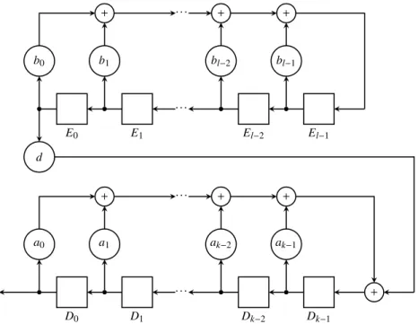
Equivalently, a preimage x ∈ F−1(y) is generated by a LFSR of order k= 2r where the feedback is summed with the output of an l-th order LFSR multiplied by d= c−12r, which produces sequence v. Similarly to concatenated LRS, we call this system a con-catenationof LFSR. Figure 4 depicts the block diagram of this concatenation.
E0 d b0 b1 + E1 · · · bl−2 + · · · El−2 bl−1 + El−1 D0 x a0 a1 + D1 · · · ak−2 + · · · Dk−2 ak−1 + Dk−1 +
Fig. 4: Diagram of two concatenated LFSR.
In conclusion, we have shown that the periods of the preimages x ∈ F−1(y) are equivalent to the periods of the concatenated LRS generated by the LFSR in Figure 4, where the disturbing LFSR is initialised with the values yr, · · · , yr+l−1. In particular,
since multiplying the terms of a LRS by a constant does not change its period, in what follows we will assume d= 1.
4
Analysis of Concatenated LRS
4.1 Sum Decomposition of Concatenated LRS
In order to study the period of the concatenated linear recurring sequence s f v giving rise to preimage x ∈ F−1(y), we first prove that it can be decomposed into the sum of two LRS: namely, sequence s and the 0-concatenation u= s f0vsatisfying the same
recurrence Equation (9) of x, but whose k initial terms u0, · · · , uk−1are set to 0.
Theorem 3. Let s= s0, s1,··· and v = v0,v1,··· be the LRS respectively satisfying
Equa-tions(11) and (10), whose initial terms are respectively s0= x0,··· , sk−1= xk−1and
v0= yr,··· ,vl−1= yr+l−1, and let x= s f v be the concatenation of s and v defined
by Equation(9), where d= 1. Additionally, let u = s f0v be the0-concatenation of
sequences s and v, where u0= u1= ··· = uk−1= 0. Then, xn= sn+ unfor all n ∈ N.
Proof. Since u0= u1= ··· = uk−1= 0, for all n ∈ {0,··· ,k − 1} it holds
sn+ un= sn+ 0 = xn .
Therefore, it remains to prove xn= sn+ unfor all n ≥ k. We proceed by induction on n.
For n= k, we have
sk+ uk= a0s0+ ··· + ak−1sk−1+ a0u0+ ··· + ak−1uk−1+ v0=
= a0x0+ ··· + ak−1xk−1+ v0= xk .
For the induction step we assume sn+un= xnfor n ≤ k. The sum sn+1+un+1is equal to:
sn+1+ un+1= a0sn−k+1+ ··· + ak−1sn+ a0un−k+1+ ··· + ak−1un+ vn−k+1=
= a0(sn−k+1+ un−k+1)+ ··· + ak−1(sn+ un)+ vn−k+1 . (12)
By induction hypothesis, sn−k+i+ un−k+i = xn−k+i for all i ∈ {1, · · · , k}. Hence, Equa-tion(12) can be rewritten as
sn+1+ un+1= a0xn−k+1+ ··· + ak−1xn+ vn−k+1= xn+1 .
u t
4.2 Characteristic Polynomial of Concatenated LRS
Theorem 3 tells us that a preimage x ∈ F−1(y) can be generated by the sum of two LRS: the LRS generated by the concatenated LFSR of Figure 4, where the disturbed LFSR is initialised to zero, and the LRS produced by the non-disturbed LFSR, that is, the lower LFSR in Figure 4 without the external feedback, initialised to the values x0,··· , xk−1.
We now show that this sum decomposition allows one to determine a characteristic polynomial of the concatenated sequence x= s f v. To this end, we first need a result proved by Chassé in [3] which concerns the generating function of the 0-concatenation u= s f0v. The proof stands on the observation that for all n ∈ N, the n-th term of u is
given by the linear combinationPn−1
coefficients ajwhich define Equation (11). In particular, we will need the values of A(0)n
for n ≥ 0, which can be computed by the following recurrence equation:
A(0)n = Pk−1 j=0ajA(0)n−k+ j , if n > 1 1 , if n= 1 0 , if n= 0 (13)
where k= 2r and A(0)n−k+ j = 0 if n − k + j < 0. Using our notation and terminology, Chassé’s result can thus be stated as follows:
Proposition 2. Let u= s f0v be the0-concatenation of the LRS s and v defined in
The-orem 3, and let V(x) be the generating function of v. Denoting by A(x) the generating function of the sequence A= {A(0)n+1}n∈N, the generating function of u is
U(x)= x · A(x) · V(x) . (14) Moreover, if a(x) ∈ Fq[x] is the characteristic polynomial of the sequence s associated
to the recurrence equation(11), then a(x) is also a characteristic polynomial of A. We now prove that the characteristic polynomial of the concatenation s f v is the product of the characteristic polynomials of s and v.
Theorem 4. Let s f v be the concatenation of LRS s and v defined by Equation (9) with d= 1, and let a(x),b(x) ∈ Fq[x] be the characteristic polynomials of s and v,
re-spectively associated to the linear recurring equations(11) and (10). Then, a(x) · b(x) is a characteristic polynomial of s f v.
Proof. By Theorem 3 the concatenation of LRS s and v can be written as s f v = s + u, where u= s f0v is the0-concatenation associated to s f v. By applying the
funda-mental identity of formal power series (Equation(5)) and Proposition 2, the following equalities hold:
S(x)=gs(x)
a∗(x) (15)
U(x)=x · gA(x) · gv(x)
a∗(x) · b∗(x) , (16)
where gs(x), gA(x) and gv(x) are polynomials whose coefficients are computed
accord-ing to the numerator in the RHS of Equation(5). Hence, the generating function of s f v is: G(x)=gs(x) a∗(x)+ x · gA(x) · gv(x) a∗(x) · b∗(x) = gs(x) · b∗(x)+ x · gA(x) · gv(x) a∗(x) · b∗(x) . (17)
By applying again the fundamental identity of formal power series to Equation(17), we deduce that the reciprocal of c(x)= a∗(x) · b∗(x) is a characteristic polynomial of s f v. Denoting by k and l the degrees of a(x) and b(x) respectively, it follows that c(x)= xk+l· a(1/x) · b(1/x), and thus the reciprocal of c(x) is
c∗(x)= xk+l· 1
xk+l· a(x) · b(x)= a(x) · b(x) . (18) Therefore, a(x) · b(x) is a characteristic polynomial of s f v. ut
Theorem (4) thus gives a characteristic polynomial for all preimages x ∈ F−1(y) of a spatially periodic configuration y ∈ FZ
q. As a matter of fact, the polynomials a(x)
and b(x) do not depend on the particular value of the block x[0,2r−1], but only on the
local rule f and on configuration y, respectively. From the LFSR point of view, this means that a preimage x ∈ F−1(y) can be generated by a single LFSR implementing the (k+ l)-th order recurrence equation
σn+k+l= c0σn+ c1σn+1+ ··· + ck+l−1σn+k+l−1 , (19)
where for all µ ∈ {0, · · · , k+ l − 1} the term cµis the µ-th convolution coefficient in the multiplication a(x) · b(x) given by
cµ=
X
i+ j=µ
aibj, for i ∈ {0,··· ,k} and j ∈ {0,··· ,l} . (20)
Additionally, the first k= 2r initial terms σ0,··· ,σk−1in Equation (19) are initialised
to the values in x[0,2r−1], while the remaining l ones are obtained using the recurrence
equation (9). Hence, by applying the fundamental identity of formal power series, the numerator of Equation (17) can also be expressed as:
g(x)= − k−1 X j=0 j X i=0 ci+k− jσixj . (21)
5
Further Results
5.1 Computing the Period of a Single Preimage
To summarise the results discussed so far, we now present a practical procedure to compute the spatial period of a single preimage. Given a LBCA F : FZ
q→ FZqwith local
rule f : F2r+1q → Fq of radius r ∈ N, a spatially periodic configuration y ∈ FZq and a
2r−cell block x[0,2r−1]∈ F2rq of a preimage x ∈ F−1(y), the procedure can be described
as follows:
1. Find the minimal polynomial b(x)= xl− bl−1xl−1· · · − b0 of the linear recurring
sequence v, where vn= yn+rfor all n ∈ N.
2. Set the characteristic polynomial a(x) associated to the inverse permutation fR,z−1 to a(x)= xk− ak−1xk−1− · · · − a0, where k= 2r and the coefficients ai are those
appearing in the recurrence equation (11).
3. Compute the polynomial g(x) given by Equation (21), and set h(x)= −g∗(x). 4. Determine the minimal polynomial of the preimage by computing
m(x)= a(x) · b(x)
gcd(a(x) · b(x), h(x)) . (22) 5. Compute the order of m(x), and output it as the period of preimage x.
For step 1, the minimal polynomial of v can be found using the Berlekamp-Massey al-gorithm[11], by giving as input to it the string composed by the first 2p elements of v, where p is the period of y (and hence the period of v as well). The time complexity of this algorithm is O(p2). Step 4 requires the computation of a greatest common divi-sor, which can be performed using the standard Euclidean division algorithm in O(n2) steps, where n= max{deg(a(x)b(x)),deg(h(x))}. Finally, the order of m(x) in step 5 can be determined by first factorizing the polynomial, for example by using Berlekamp’s algorithm[1] which has a time complexity of O(D3), where D is the degree of m(x), if the characteristic ρ of Fqis sufficiently small. Once the factorization of m(x) is known,
ord(m(x)) can be computed using the following theorem proved in [9]:
Theorem 5. Let m(x) ∈ Fq[x] be a polynomial having positive degree and such that
m(0) , 0. Let m(x) = a ·Qn
i=0fi(x)bibe the canonical factorization of m(x), where a ∈ Fq,
b1,··· ,bn∈ N and f1(x), · · · , fn(x) ∈ Fq[x] are distinct monic irreducible polynomials.
Then ord(m(x))= eρt, whereρ is the characteristic of Fq, e is the least common multiple
of ord( f1(x)), · · · , ord( fn(x)) and t is the smallest integer such that ρt≥ max (b1,··· ,bn).
Notice that Theorem 5 depends on the knowledge of the orders of the irreducible poly-nomials involved in the factorization of m(x). A method to determine the order of an ir-reducible polynomial is also described in [9], which relies on the factorization of qD− 1. There exist several factorization tables for numbers in this form, especially for small values of q (see for example [4]).
We now present a practical application of the procedure described above. The com-putations in the following example have been carried out with the computer algebra system MAGMA.
Example 1. Let F : FZ
2→ FZ2 be the LBCA with local rule f : F 3
2→ F2of radius r= 1,
defined as f (x1, x2, x3)= x1+ x2+ x3for all (x1, x2, x3) ∈ F32, which is the elementary
rule 150. Let y ∈ FZ
2 be a spatially periodic configuration of period p= 4 generated
by the block y[0,3]= (0,0,1,1), and let x[0,1]= (1,0) be the initial 2-cell block of a
preimage x ∈ F−1(y). Since r= 1, sequence v is generated by block v[0,3]= (0,1,1,0).
Feeding the string (0, 1, 1, 0, 0, 1, 1, 0) to the Berlekamp-Massey algorithm yields the polynomial b(x)= x3+ x2+ x +1, while the characteristic polynomial associated to rule 150 is a(x)= x2+ x + 1. Hence, it follows that c(x) = a(x) · b(x) = x5+ x3+ x2+ 1 is a characteristic polynomial of the preimage. Since the first 5 elements of preimage x are 1, 0, 1, 0, 0, the initialisation polynomial of Equation (21) is g(x)= x4+ x3+ 1, from which we deduce that h(x)= x4+ x+1. Considering that h(x) is irreducible, the greatest common divisor of c(x) and f (x) is 1, and thus by Equation (22) c(x) is also the minimal polynomial of the preimage. The factorization of c(x) is (x+ 1)3(x2+ x + 1), and the orders of x+ 1 and x2+ x + 1 are respectively 1 and 3, from which it follows that the least common multiple e is 3. Finally, the smallest integer t such that 2t≥ 3 is t= 2. Therefore, by applying Theorem 5 the period of preimage x is e2t= 12. Figure 5 shows
the actual value of the block x[0,11]which generates preimage x.
5.2 Characterisation of Periods When a(x) and b(x) Are Irreducible
As a further application of Theorem 4, we now show a complete characterisation of the periods of x ∈ F−1(y) in the special case where the characteristic polynomials a(x)
0 y0 · · · 0 y1 1 y2 1 y3 0 y4 0 y5 1 y6 1 y7 0 y8 0 y9 1 y10 1 y11 0 y12 0 y13 · · · 0 x1 1 x0 · · · 1 x2 0 x3 0 x4 0 x5 0 x6 1 x7 0 x8 1 x9 1 x10 1 x11 1 x12 0 x13 · · ·
Fig. 5: Block x[0,11] which generates preimage x ∈ F−1(y) under rule 150, computed
using case (a) of Equation (1). Notice that (x12, x13)= (x0, x1) and (y12,y13)= (y0,y1).
Hence, for n ≥ 12 and n < 0 the preimage will periodically repeat itself.
and b(x) are irreducible. To this end, we first report an additional theorem proved in [9] which concerns the sum of families of LRS.
Theorem 6. Let f1(x), f2(x) ∈ Fqbe non-constant monic polynomials, and let S( f1(x))
and S( f2(x)) be the families of LRS whose characteristic polynomials are respectively
f1(x) and f2(x). Denoting by S ( f1(x))+ S ( f2(x)) the family of all LRS σ+ τ where
σ ∈ S ( f1(x)) and τ ∈ S ( f2(x)), it follows that S ( f1(x))+ S ( f2(x))= S (c(x)), where c(x)
is the least common multiple of f1(x) and f2(x).
Our characterisation result, which is analogous to Theorem 2, is the following: Theorem 7. Let F : FZ
q → FqZbe an LBCA having local rule f : F2r+1q → Fq, and let
a(x)= xk− ak−1xk−1− · · · − a0∈ Fq[x] be the characteristic polynomial associated to
the inverse permutation fR,z−1, where k= 2r, a0,··· ,ak−1are the coefficients appearing in
Equation(11) and ord(a(x))= e. Further, let y ∈ FZ
qbe a spatially periodic configuration
of period p> 1, and let b(x) be the minimal polynomial of sequence v, where vn= yn+r
for all n ∈ N. If a(x) and b(x) are both irreducible and a(x) , b(x), then F−1(y) contains one configuration of period p and qk− 1 configurations of period m, where m is the least common multiple of e and p.
Proof. By Theorem(4), a(x) · b(x) is a characteristic polynomial of the qkpreimages in F−1(y). Denote by S (a(x)) and S (b(x)) the sets of LRS having characteristic polynomi-als a(x) and b(x), respectively. Since a(x) and b(x) are both irreducible and a(x) , b(x), by Theorem 6 it follows that S(a(x) · b(x))= S (a(x))+S (b(x)). Hence, F−1(y) is a subset of S(a(x))+ S (b(x)), and as a consequence every preimage x ∈ F−1(y) can be written as x= σ + τ, where σ ∈ S (a(x)) and τ ∈ S (b(x)). In particular, by applying Theorem 2 it results that S(a(x)) is composed by one sequence of period 1 and qk− 1 sequences of period e, while since p> 1 the sequence τ is necessarily one of the ql− 1 sequences of period p of S(b(x)), where l is the degree of b(x). Therefore, by making all possible sums forσ ranging in S (a(x)), Theorem 1 yields that F−1(y) is composed by one con-figuration having period p, which is the preimage x= σ+τ where σ has period 1, while the period of all the remaining qk− 1 configurations is the least common multiple of e
and p. ut
6
Conclusions
In this work, we studied the relation between the periods of spatially periodic configura-tions of LBCA and the periods of their preimages, characterising the latter as
concatena-tions of linear recurring sequences. We remark that Theorem 4 can be straightforwardly generalised to the case x(t)∈ F−t(y), i.e. preimages of y with respect to the t-th iterate of the CA, where t ∈ N. Indeed, it can be shown that a(x)t· b(x) is a characteristic polyno-mial of x(t), which is thus generated by a “cascade” of concatenated LFSR where each LFSR is initialised to a block x(i)[0,2r−1] of an intermediate preimage x(i)∈ F−i(y), for i ∈ {1, · · · , t}. Of course in this case we have to take into account the fact that the running time of the procedure described in Section 5.1 grows exponentially in the degree D of the minimal polynomial m(x), since it depends on the factorization of qD− 1.
We conclude by discussing some possible future directions of research on the sub-ject. A first idea is to generalise the results presented in this paper to nonlinear BCA, where the preimages are generated by a Nonlinear Feedback Shift Register (NFSR) dis-turbed by the LFSR which generates configuration y. We remark that this concatenation is also the main primitive upon which the stream cipher Grain is based [8]. Hence, finding a general method to study the periods of preimages of nonlinear BCA could also be useful to cryptanalyse this cipher. This study could be further generalised to generic surjective CA. In this regard, a possible starting point could be a result reported in [5], which implies that if F : FZ
q→ FZqis a surjective linear CA, then there exists t ∈ N
such that the t-th iterate Ftis bipermutive. Finally, a further extension of this research would be to analyse the periods of spatially periodic configurations in the case of multi-dimensional cellular automata, by considering suitable notions of bipermutivity such as the ones introduced in [6].
References
1. Berlekamp, E.R.: Factoring polynomials over finite fields. Bell Syst. Tech. J. 46, 1853–1859 (1967)
2. Cattaneo, G., Finelli, M., Margara, L.: Investigating topological chaos by elementary cellular automata dynamics. Theor. Comp. Sci. 244, 219–241 (2000)
3. Chassé, G.: Some remarks on a LFSR “disturbed” by other sequences. In: Cohen, G., Charpin. P. (eds.) EUROCODE ’90. LNCS vol. 514, pp. 215–221. Springer, Heidelberg (1991)
4. The Cunningham Project, http://homes.cerias.purdue.edu/~ssw/cun/index.html 5. Dennunzio, A., Di Lena, P., Formenti, E., Margara, L.: On the directional dynamics of
addi-tive cellular automata. Theor. Comput. Sci. 410, 4823–4833 (2009)
6. Dennunzio, A., Formenti, E., Weiss, M.: Multidimensional cellular automata: closing prop-erty, quasi-expansivity, and (un)decidability issues. Theor. Comput. Sci. 516, 40–59 (2014) 7. Hedlund, G.A.: Endomorphisms and Automorphisms of the Shift Dynamical Systems.
Math-ematical Systems Theory 7(2), 138–153 (1973)
8. Hell, M., Johansson, T., Meier, W.: The Grain Family of Stream Ciphers. In: Robshaw, M., Billet, O. (eds.) New Stream Ciphers Designs. LNCS vol. 4986, pp. 179–190. Springer, Hei-delberg (2008)
9. Lidl, R., Niederreiter, H.: Introduction to finite fields and their applications. Cambridge Uni-versity Press, Cambridge (1994)
10. Mariot, L., Leporati, A.: Sharing Secrets by Computing Preimages of Bipermutive Cellular Automata. In: Was, J., Sirakoulis, G.Ch., Bandini, S. (eds.): ACRI 2014. LNCS vol. 8751, pp. 417–426. Springer, Heidelberg (2014)
11. Massey, J.L.: Shift-register synthesis and BCH decoding. IEEE Trans. Inf. Theory 15, 122– 127 (1969)


![Fig. 5: Block x [0,11] which generates preimage x ∈ F −1 (y) under rule 150, computed using case (a) of Equation (1)](https://thumb-eu.123doks.com/thumbv2/123doknet/13267652.397239/14.892.269.649.179.256/fig-block-generates-preimage-rule-computed-using-equation.webp)
