HAL Id: hal-00862399
https://hal.archives-ouvertes.fr/hal-00862399v2
Submitted on 15 Nov 2013
HAL is a multi-disciplinary open access
archive for the deposit and dissemination of sci-entific research documents, whether they are pub-lished or not. The documents may come from teaching and research institutions in France or abroad, or from public or private research centers.
L’archive ouverte pluridisciplinaire HAL, est destinée au dépôt et à la diffusion de documents scientifiques de niveau recherche, publiés ou non, émanant des établissements d’enseignement et de recherche français ou étrangers, des laboratoires publics ou privés.
measurements with toroidal harmonics for equilibrium
reconstruction in a Tokamak
Blaise Faugeras, Jacques Blum, Cédric Boulbe, Philippe Moreau, Eric Nardon
To cite this version:
Blaise Faugeras, Jacques Blum, Cédric Boulbe, Philippe Moreau, Eric Nardon. 2D interpolation and extrapolation of discrete magnetic measurements with toroidal harmonics for equilibrium reconstruc-tion in a Tokamak. Plasma Physics and Controlled Fusion, IOP Publishing, 2014, 56, pp.114010. �hal-00862399v2�
magnetic measurements with toroidal harmonics for
equilibrium reconstruction in a tokamak
Blaise Faugeras1, Jacques Blum1, Cedric Boulbe1, Philippe
Moreau2 and Eric Nardon2
1Laboratoire J.A. Dieudonn´e, UMR 7351, Universit´e Nice Sophia-Antipolis, Parc Valrose, 06108 Nice Cedex 02, France
2CEA, IRFM, F-13108, Saint-Paul-lez-Durance, France E-mail: Blaise.Faugeras@unice.fr
Abstract. We present a method based on the use of toroidal harmonics and on a modelization of the poloidal field coils and divertor coils for the 2D interpolation and extrapolation of discrete magnetic measurements in a tokamak. The method is generic and can be used to provide Cauchy boundary conditions needed as input by a fixed domain equilibrium reconstruction code like Equinox [1]. It can also be used to extrapolate the magnetic measurements in order to compute the plasma boundary itself. The proposed method and algorithm are detailed in the paper and results from numerous numerical experiments are presented. The method is foreseen to be used in the real time plasma control loop on the WEST tokamak [2].
1. Introduction
Equilibrium reconstruction codes are fundamental for the analysis and the control of fusion experiments in a tokamak [3]. The state variable of interest in the modelization of such an equilibrium under the usual axisymmetric assumption is the poloidal flux ψ(r, z)
which is related to the poloidal magnetic field by the relation B = 1
r(−∂zψ, ∂rψ) in the cylindrical coordinate system (r, φ, z). The basic inputs used to achieve the numerical reconstruction of the equilibrium are magnetic measurements taken at several locations surrounding the vacuum vessel.
Basically equilibrium codes can be of two types. The first one is the full domain type in which the reconstruction is performed in the whole right half plane (r > 0) and relies on the use of Green’s functions. A drawback of this method is that nonlinear ferromagnetic structures which can be present in certain tokamaks are complicated to deal with. An iron model has to be introduced [4] and these codes can hardly run in real time. The second type of code is the bounded domain one in which computations are performed in a fixed domain containing the plasma but restricted to a limited
region. A difficulty is that Cauchy boundary conditions (g = ψ, h = ∂nψ) have to
be provided on a fixed closed contour defining the boundary of the computation domain (this contour, called Γ in the remaining part of this paper, can link some of the B probes for example). These boundary conditions have to be computed from the discrete magnetic measurements. If these measurements are numerous enough and regularly located on a smooth contour a direct linear interpolation can be considered [5, 6]. However this method is not robust in case of defective sensors. Morevover it cannot be used in today’s machines like JET in which the measurement points are scattered in some annular region surrounding the vacuum vessel. Another approach which can be considered is to use the plasma boundary identification code of a particular machine if it exists. Such a code will in fact compute the poloidal flux ψ in the vacuum surrounding the plasma and can be used to evaluate ψ and its normal derivative on any given fixed closed contour Γ. This is the approach followed until now for the equilibrium reconstruction code Equinox [1]. The computations rely on the boundary conditions g and h provided by the plasma boundary reconstruction codes Xloc at JET [7, 8] and the Apolo code at Tore Supra [9]. The main drawback of this approach is that these two
boundary reconstruction codes are extremely machine dependent and not transportable to a generic platform such as the ITM [10]. Moreover concerning the particular case of Tore Supra a new numerical method has to be developped since the machine is going to be upgraded to WEST [2].
The aim of this paper is to investigate the possibility of using toroidal harmonics to perform the 2D interpolation and extrapolation of magnetic measurements in an annular domain surrounding the plasma to compute Cauchy boundary conditions on a given fixed closed contour Γ in order to be able to run in a second step an equilibrium reconstruction code such as Equinox in the bounded domain limited by Γ. Actually at a given instant in time the fictitious inner boundary of the annular domain could be defined as being the plasma boundary itself and the data interpolation problem is very closely connected to the ill-posed inverse problem of the identification of the plasma
boundary. The latter is a Cauchy problem for the elliptic equation ∆∗
ψ = 0 and various
solution methods have been proposed to solve it, compute ψ in the vacuum surrounding the plasma and identify the plasma boundary (see [11] for a review). The ill-posedness of the problem usually imposes the use of a regularization technique and an apriori representation of plasma current density and the flux it generates, called the internal solution, for example using filaments of current, or a fictious current sheet, or also a decomposition in toroidal harmonics. The latter seems particularly attractive since these functions provide explicit solutions to the equation ∆∗
ψ = 0. Toroidal harmonics
[12, 13] were used in a number of papers in the plasma physics literature in the 80’s and 90’s [14, 15, 16, 17, 18, 19, 20] and more recently in [21].
Apart from [16] and [21] authors using toroidal harmonics do not use any regularization procedure. Our point of view is that the small number of harmonics needed to represent the flux in the vacuum is in itself a regularizing procedure. Our numerical experiments confirm this point. In fact the number of toroidal harmonics used to represent the internal solution in some way can be seen as the regularization parameter. A too small number might lead to a smooth solution possibly not fitting the data very well and not giving a very accurate plasma boundary, whereas a too large number might lead to an irregular solution well fitting the data but giving an irregular plasma boundary.
Another ingredient of the method to which the solution is quite sensitive is the location of the pole of the toroidal coordinates system. Actually together with the number of internal toroidal harmonics it is the only parameter of the internal solution which can be tuned and curiously it is generally kept fixed in the literature apart from [19] in which an optimization method is proposed to identify a proper location of the pole. In this paper we propose two simple methods to do so.
Finally in order to represent the flux ψ in the vacuum some authors use a pure decomposition in toroidal harmonics [14, 15, 16, 20] whereas others add a term coming from the modelization of the flux generated by the poloidal field coils [17, 19]. In this paper we discuss this point together with the impact of the presence of nonlinear ferromagnetic material. Our numerical experiments show that it is important to take
into account the divertor coils.
The paper is organized as follows. In the next section we introduce notations for a number of domains and contours which are needed. Section 3 deals with the decomposition of the flux in toroidal harmonics. In section 4 the proposed numerical algorithm is presented and in the last section a number of numerical results are presented.
2. Mathematical setting
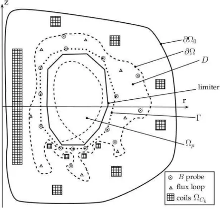
In order to get into the details of this work we first need to briefly recall the equilibrium reconstruction problem and introduce a number of contours and domains. Therefore a schematic representation of a poloidal cross-section of a tokamak is shown on Fig. 1 and described below.
The unknown plasma free boundary domain is noted Ωp. The plasma boundary
is the isoflux line whose value is defined either by the contact with the limiter or as a magnetic separatrix (hyperbolic line with an X-point represented by the dashed line inside the limiter contour in Fig. 1). Poloidal field coils and divertor coils are noted ΩCk. Poloidal field probes measure the local value of the poloidal magnetic field, flux loops and saddle loops measure the local value of the flux ψ. Flux and saddle loops, represented by triangles, and B probes, represented by cross-circles, are shown surrounding the limiter contour. All these measurements points can be included into a fictitious annular domain D which neither contains the coils nor the plasma. The inner boundary of D can for example be chosen to be the limiter contour. The presence of divertor coils can impose the choice of a somehow tortured outer boundary (dashed line labelled ∂Ω). The
outer boundary of D also defines a domain Ω including D, Ωp and the vacuum region
lying between the plasma and D. Eventually all these different domains are included in
the larger domain Ω0 outside of which nonlinear magnetic material like iron might be
present. Its boundary is noted ∂Ω0.
Depending on the domain the poloidal flux satisfies the partial differential equation −∆∗ ψ = 0 in D (1) or −∆∗ ψ = jp(ψ, r)χΩp in Ω (2) or −∆∗ ψ = jp(ψ, r)χΩp+ X k jCkχΩCk in Ω0 (3)
where the differential operator ∆∗ = ∂ ∂r( 1 µ0r ∂ ∂r) + ∂ ∂z( 1 µ0r ∂ ∂z),
is linear, the right hand sides represents the toroidal component of the local current density and χ is the indicator function. If iron is present outside Ω0 (like for JET and
Figure 1. Schematic representation of a poloidal cross-section of a tokamak. See the text for details.
Tore Supra) µ0 is no longer a constant but a function of |B| and the operator ∆∗becomes nonlinear. This is why we restrict ourselves to Ω0 where ∆∗ is linear. In Ω0\{ΩpS ΩCk} the current is null. In the coils ΩCk the densities jCk are measured and known. In the
plasma Ωp the current density is unknown but according to Grad-Shafranov equation
takes the form
jp(ψ, r) = rp′(ψ) + 1 µ0r (f f′ )(ψ) (4) in which p′ and f f′
are unknown functions to be identified by an equilibrium reconstruction code.
As explained in the Introduction one of our goals is to compute Cauchy conditions
(g = ψ, h = ∂nψ) on contour Γ in order to provide inputs to the reconstruction code
Equinox. Indeed let us recall that this code solves the following problem:
Find functions A and B defined on [0, 1] which minimize the following regularized cost function J(A, B) = Z Γ (∂nψ− h)2ds+ ǫ( Z 1 0 (A′′ (x))2+ (B′′ (x))2dx) where ψ satisfies −∆∗ ψ = λ(r r0 A( ¯ψ) + r0 r B( ¯ψ))χΩp(ψ), in DΓ ψ = g on Γ
Here λ is a scaling factor, r0 is a constant, A and B are related to p′ and f f′, ¯ψ is a
normalized flux and DΓ is the domain contained inside Γ. Equinox implements a finite
element discretization method and identifies the full equilibrium (plasma boundary and
current density) in the fixed domain DΓ. This computation completely relies on the
boundary conditions g and h deduced from the magnetic measurements.
3. Decomposition of the poloidal flux ψ in the annular domain D
In this section we recall the principle of the decomposition of the flux in toroidal harmonics in the region D. Moreover we show that the non linearity induced by the presence of iron outside Ω0 does not restrict the possibility of using a modelization of the flux generated by the different coils.
3.1. Toroidal harmonics
The toroidal coordinates system [13, 22] or bipolar coordinates system (if we ignore the angular toroidal variable) (ζ, η) ∈ IR+∗ × [0, 2π] about the pole F0 = (r0, z0) is related to the cylindrical coordinates system (r, z) by
r = r0sinh ζ
cosh ζ − cos η and z − z0 =
r0sin η cosh ζ − cos η
In what follows we assume that F0 lies inside the region surrounded by the annular
domain D and more precisely inside the plasma domain where the homogeneous
equation, −∆∗
ψ = 0, is not satisfied. In the domain D this equation is satisfied.
It is known that explicit solutions to this equation in an annular domain can be found in toroidal coordinates using a quasi separation of variables technique (see [23, 24] for details on the computations). Moreover the family of solutions found is complete [24, 21]. That is to say that, given any regular enough Dirichlet boundary condition u on ∂D, the solution to the boundary value problem
( −∆∗
ψ = 0 in D
ψ = u on ∂D (5)
can be uniquely decomposed as ψ = ψext+ ψint ψext = r0sinh ζ √ cosh ζ − cos η× [ ∞ X n=0 aenQ1n−1/2(cosh ζ) cos(nη) + ∞ X n=1 benQ1n−1/2(cosh ζ) sin(nη)] ψint = r0sinh ζ √ cosh ζ − cos η× [ ∞ X n=0 ainPn−1/21 (cosh ζ) cos(nη) + ∞ X n=1 binPn−1/21 (cosh ζ) sin(nη)] (6)
where P1
n−1/2 and Q1n−1/2 are the associated Legendre functions of first and second kind,
of degree one and half integer order [25], also called toroidal harmonics when evaluated at point cosh ζ. Functions P1
n−1/2have a singularity when ζ → ∞ that is to say at point
F0 and therefore ψint represents the flux generated by currents flowing inside D. On the contrary functions Q1
n−1/2 are singular when ζ → 0 that is to say on the axis r = 0 and
therefore ψext represents the flux generated by currents flowing outside D. 3.2. Including information from the knowledge of the currents in the coils
Let us denote by x = (r, z) a point in the poloidal plane. For any scalar fields ψ and
φ on Ω, two integrations by parts of the quantity φ∆∗
ψ lead to the so called Green’s
second identity (or Green’s theorem) Z Ω (φ∆∗ ψ− ψ∆∗ φ)dx = Z ∂Ω 1 µ0r (∂φ ∂nψ− ∂ψ ∂nφ)ds (7)
Let ¯x ∈ D and G(x, ¯x) be the free space Green function which satisfies
−∆∗
G(x, ¯x) = δ(x − ¯x) in the whole half plane r > 0 and G(x, ¯x) → 0 when |x| → ∞ or r → 0.
The important point here is that even if the region external to Ω0contains nonlinear materials such as iron, the restriction of G to Ω can still be used as function φ in Eq. (7). If ψ is chosen to be the solution to Eq. (2) one gets
ψ(¯x) = Z Ωp jp(ψ(x), r)G(x, ¯x)dx+ Z ∂Ω 1 µ0r (∂G ∂n(x, ¯x)ψ(x)− ∂ψ ∂n(x)G(x, ¯x))ds(8)
and this leads again to a decomposition of the type ψ = ψint+ ψext with
ψint(¯x) = R Ωpjp(ψ(x), r)G(x, ¯x)dx ψext(¯x) = Z ∂Ω 1 µ0r (∂G ∂n(x, ¯x)ψ(x) − ∂ψ ∂n(x)G(x, ¯x))ds (9) ψint is another expression for the flux generated by currents running inside D and ψext
for those running outside. Moreover Green’s theorem can also be applied in Ω0 (the
region including the plasma and the coils). One then gets the following expression for ψ in D: ψ = ψint+ ψext+ ψC with
ψint(¯x) = R Ωpjp(ψ(x), r)G(x, ¯x)dx ψext(¯x) = Z ∂Ω0 1 µ0r (∂G ∂n(x, ¯x)ψ(x) − ∂ψ ∂n(x)G(x, ¯x))ds ψC(¯x) = X k Z Ck jCkG(x, ¯x)dx (10)
where ψC represents the contribution of the coils to the total flux. In the annular domain D, ˜ψ = ψ − ψC = ψint+ ψext still satisfies
( −∆∗˜ ψ = 0 in D ˜ ψ = ψ|∂D− ψC|∂D on ∂D (11) and can thus be decomposed in toroidal harmonics.
This shows that the knowledge of the currents jCk in the coils can be used in the representation of the flux in the region D in the presence or absence of iron outside
Ω0. In fact if the coils are located very close to the measurement points such as the
divertor coils are it is necessary to modelize them. Their contribution to the flux in
D can theoretically be written as a series of toroidal harmonics but many of them are
needed in practice. This can be critical compared to the number of measurements and the numerical resolution of the problem might become difficult.
4. Numerical method
Let us now present the numerical method which we implemented. At each discrete time step during a discharge the magnetic measurements available are of three types:
• Flux loops provide Nf flux measurements at points xfi such that ψimeas≈ ψ(x f i)
• Saddle loops provide Nsflux variations measurements between two points such that
δiψmeas ≈ ψ(x1i) − ψ(x2i)
• B probes provide NB measurements of the poloidal field at points xBi and directions di such that Bimeas ≈ B(xBi ).di
The first step of the algorithm consists in substracting from the measurements a numerical approximation of the contribution from the coils.
˜ ψimeas = ψmeas i − ˆψC(xfi), for i = 1, . . . Nf
δiψ˜meas = δiψmeas− ( ˆψC(x1i) − ˆψC(x2i)), for i = 1, . . . Ns ˜
Bimeas = Bmeas
i − ˆBC(xBi ).di, for i = 1, . . . NB
(12)
Here the contribution from each coil Ck is computed as follows. The known current
density is given as jCk =
Ik
Sk where Ik is the total current in the coil and Sk its surface. The coil is divided into nk subcoils Ck,l of equal surface Snk
k and center ck,l on which the integrals are numerically evaluated as
Z Ck,l Ik Sk G(x, ¯x)dx ≈ Ik nk G(ck,l,x)¯ (13)
This in fact consists in considering the contribution of the coils as a sum of the contributions from filaments of current
ˆ ψC(¯x) = X k X l Ik nk G(ck,l,x)¯ (14)
The second step consists in truncating the toroidal harmonics expansion of ˜ψ to approximate it by ˆ ψ = ψˆext+ ˆψint ˆ ψext = r0sinh ζ √ cosh ζ − cos η× [ ne a X n=0 aenQ1n−1/2(cosh ζ) cos(nη) + ne b X n=1 benQ1n−1/2(cosh ζ) sin(nη)] ˆ ψint = r0sinh ζ √ cosh ζ − cos η× [ ni a X n=0 ainPn−1/21 (cosh ζ) cos(nη) + ni b X n=1 binPn−1/21 (cosh ζ) sin(nη)] (15)
and evaluate each of the terms in the expansion of ˆψ and of the associated field ˆB at the different measurement points in order to form a least square cost function
J(u) = Nf X i=1 ( ˆψi(u) − ˜ψimeas)2 σ2 f + Ns X i=1 (δiψˆ(u) − δiψ˜meas)2 σ2 s + NB X i=1 ( ˆBi(u) − ˜Bimeas)2 σ2 B (16) depending on u= (ae0, . . . , aene a, b e 1, . . . , bene b, a i 0, . . . , aini a, b i 1, . . . , bini b)
the unknown coefficients of the expansion in toroidal harmonics. The weights σf, σs and
σB correspond to the assumed measurement errors. J is quadratic in u and is minimized
by solving the associated normal equation to find the optimal set of coefficients uopt.
In these computations the expressions for ˆψC and ˆBC are explicit [26]. The
expression for ˆBis also explicit. The numerical evaluation of half integer order associated Legendre functions is not straightforward. We use the algorithm and the computer routine DTORH1 provided with [27]. This code enables an accurate and fast evaluation of the set Pm
n−1/2(x), Qmn−1/2(x) for real x > 1, integers m ≥ 0 and n = 0, · · · N.
Once uopt is computed an approximation of the flux can be obtained at any point
of the vacuum surrounding the plasma by ψ(x) = ˆψ(x) + ˆψC(x). In particular one can
evaluate ψ and its normal derivative on a fixed closed countour Γ in order to provide Cauchy boundary conditions to a fixed bounded domain equilibrium reconstruction code. Of course one can also identify the plasma boundary as the largest closed flux surface inside the limiter contour.
Such a procedure provides meaningful results if the pole F0 lies inside the unknown plasma region and not too close from the boundary. The most natural choice is to put the pole at the location of the magnetic axis but as the plasma boundary it is unknown. Thus we propose the following procedure. At the first time step the pole is located at
(r0,0) where r0 is the major radius of the tokamak. Then at time step tn+1 the pole
is located at the position of the magnetic axis computed at the previous time step tn.
This magnetic axis position is computed exactly if an equilibrium reconstruction code like Equinox is run at each time step. If this is not the case and one is only interested in the plasma boundary identification problem, or by an equilibrium reconstruction at
a given instant in time it can be approximated by the current center (rc, zc) defined as moments of the plasma current density [28, 11]. These quantities can be precisely computed as integrals on the contour Γ at every point of which the flux ψ and the field
B can be evaluated: Ip := Z DΓ jpdx = Z Γ 1 µ0 Bsds zcIp := Z DΓ zjpdx = Z Γ 1 µ0(−r log rBn + zBs)ds r2cIp := Z DΓ r2jpdx= Z Γ 1 µ0 (2rzBn+ r2Bs)ds 5. Numerical results
5.1. Twin experiments for WEST
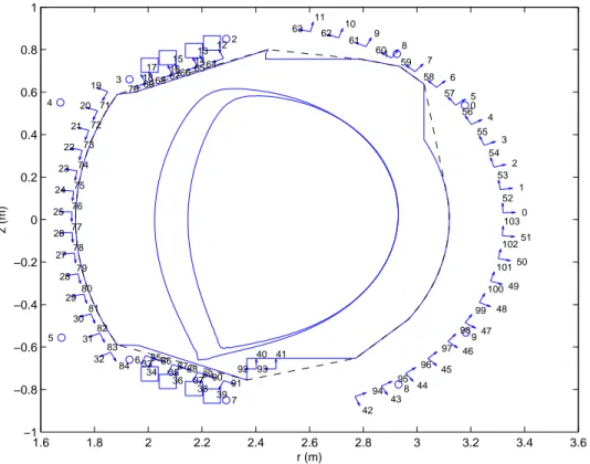
In view of the upgrade of the tokamak Tore Supra to WEST we have conducted several numerical experiments to test the method. The code Cedres++ [29] is run to simulate four WEST equilibria. In the first case the X-point position is very close to the limiter whereas in the second one the plasma is smaller. Configurations 3 and 4 are limiter configurations. From these simulations the equivalent of magnetic measurements are extracted: 10 flux loops measurements and 104 Bprobes measurements (see Fig 2). The reconstruction of the plasma boundary and the equilibrium can then be performed using these measurements as inputs as well as the currents running in the coils. Using the notations of Eq. (16) we take Nf = 10, σf = 10−3 [W b2π] and NB = 104, σB = 10−3 [T ].
Let us first concentrate on the reconstruction of the flux in vacuum for case 1 with the algorithm using toroidal harmonics (TH). Unless specified we always take into account the values of the currents in the coils. Here we want to reconstruct a single equilibrium and thus do not have a priori at our disposal the knowledge of the magnetic axis position. As described in section 4 we proceed in 2 steps. First run TH setting the pole of the toroidal coordinate system to P0 = (r0,0), compute the current center P1 = (rc, zc) and re-run TH setting the pole to these new coordinates. This mimics the fact that during a whole pulse reconstruction the current center at the previous time step would play the role of P0and if P1 is too far from P0 then the pole of the coordinate system is modified.
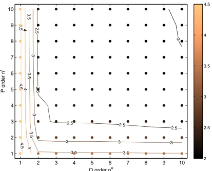
A first natural question which has to be answered is how many toroidal harmonics should be used to represent the flux ψ in the vacuum. In all the computations we choose
the maximum order of the toroidal harmonics used in Eq. (15) to be ne := ne
a = neb and
ni := ni
a= nib. From Fig. 3 it appears that the value of the cost function at the optimal point, which is an indicator of the quality of the fit to the measurements, decreases very
rapidly as we increase the maximum order from ne= ni = 1 to 4. Above this value the
benefit of adding new degrees of freedom is much less significant and the plot shows an almost flat region for orders greater than 4.
1.6 1.8 2 2.2 2.4 2.6 2.8 3 3.2 3.4 3.6 −1 −0.8 −0.6 −0.4 −0.2 0 0.2 0.4 0.6 0.8 1 0 1 2 3 4 5 6 7 8 9 0 1 2 3 4 5 6 7 8 9 10 11 12 13 14 15 16 17 18 19 20 21 22 23 24 25 26 27 28 29 30 31 32 33 34 35 36 37 38 39 40 41 42 43 44 45 46 47 48 49 50 51 52 53 54 55 56 57 58 59 60 61 62 63 64 65 66 67 68 69 70 71 72 73 74 75 76 77 78 79 80 81 82 83 84 85868788 8990 91 92 93 94 95 96 97 98 99 100 101 102 103 r (m) z (m)
Figure 2. Poloidal section of the WEST tokamak. The two plasma boundaries correspond to case 1 (large plasma) and case 2 (smaller plasma). The Bprobes represented by arrows are numbered from 0 to 103 and the flux loops represented by small circles are numbered from 0 to 9. The four bottom divertor coils are shown as well as the top ones. The limiter contour is also plotted as well as its convex hull (dashed line) which will be used as contour Γ that is to say the boundary of the computation domain for the equilibrium reconstruction code Equinox.
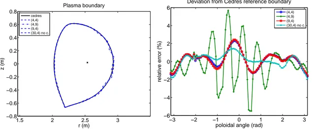
As a consequence we make the choice ne = ni = 4. This corresponds to the
minimum number of degrees of freedom needed to obtain a good fit to the measurements. Numerical values for the optimal cost and corresponding root mean square (rms) errors
are given for different choices of ne and ni in Table 1. The corresponding computed
plasma boundaries are also shown on Figure 4. As already mentioned adding interior functions (column (4, 9)) or exterior functions (column (9, 4)) does not significantly
modify the rms. However in the first case it deterioriates the plasma boundary
reconstruction (Fig. 4). This is due to the fact that interior functions are involved
with the ill-posed character of the inverse boundary reconstruction problem. The
only regularization mechanism lies in the small number of toroidal harmonics used to represent the flux. The blow up of the interior harmonics accentuates with their order and the zone where the computed solution is not relevant spreads around the pole of the coordinate system even reaching the plasma boundary in this case. This phenomenum disappears in the plasma boundaries computed by Equinox in all cases (see Figure 6) and this is due to the fact that the reconstruction of the boundary is not an ill-posed
2 2.5 2.5 2.5 2.5 2.5 3 3 3 3 3 3.5 3.5 3.5 3.5 3.5 4 4 4 4.5 4.5 4.5 Q order ne P order n i 1 2 3 4 5 6 7 8 9 10 1 2 3 4 5 6 7 8 9 10 2 2.5 3 3.5 4 4.5
Figure 3. Contour and scatter plot of log(J(uopt)) as a function of the maximum order of the associated Legendre functions of first kind ni and second kind neused for the representation of the flux.
inverse problem in Equinox in which the equation for ψ is solved also in the plasma and the free boundary problem is a particular non linearity of the model.
The last column of Table 1 shows the interest of using a modelization of the flux generated by the divertor and poloidal field coils. If we do not use these informations in this particular case the value of ne has to be taken of at least 30 to achieve a fit to the measurements comparable to the one obtain with the choice (4, 4).
(ne, ni) (4, 4) (4, 9) (9, 4) (30, 4) no c.
cost J(uopt) 2.783e+02 1.666e+02 2.004e+02 3.352e+02
rms B [T ] 1.614e-03 1.233e-03 1.343e-03 1.624e-03
rms Flux [W b
2π] 5.814e-04 6.663e-04 7.832e-04 1.657e-03
Table 1. Minimization results for the default choice (ne= 4, ni= 4), as well as choices (4, 9), (9, 4) and (30, 4) without using any representation of the flux generated by the divertor and poloidal field coils (no c.)
Figure 5 shows the fit to the measurements for the choice ne = ni = 4. It appears
that the largest errors on the Bprobes measurements happen for those in the range 32-40 and 84-92 which correspond to the ones located close to the X-point. These numerical experiments therefore suggest that if some sensors could be added in the design of WEST, it is desirable to put them if possible in the region of the divertor.
From Table 2 it can be seen that the reconstruction of the Xpoint position is
quite accurate (up to a few mm) with the default choice (ne = 4, ni = 4). More
1.5 2 2.5 3 −0.8 −0.6 −0.4 −0.2 0 0.2 0.4 0.6 0.8 r (m) z (m) Plasma boundary cedres (4,4) (4,9) (9,4) (30,4) no c. −3 −2 −1 0 1 2 3 −6 −4 −2 0 2 4 6
poloidal angle (rad)
relative error (%)
Deviation from Cedres reference boundary
(4,4) (4,9) (9,4) (30,4) no c.
Figure 4. Left: Plasma boundaries. Boundaries computed with (ne = 4, ni = 4) or (ne = 9, ni = 4) and (ne = 30, ni = 4) without any PF coils modelization (no c.) are almost superimposed with the reference boundary computed with Cedres. The boundary computed with (ne= 4, ni= 9) shows some irregularity
Right: Corresponding relative deviation from Cedres++ boundary,
100(ρ − ρCedres)/ρCedresas a function of the poloidal angle θ. The center of the polar coordinate system (ρ, θ) is the magnetic axis from Cedres++ (shown on left figure).
0 20 40 60 80 100 0 1 2 3 4 5 6 #Bcoil error B (mT)
Absolute errors on Bprobes reconstruction
0 1 2 3 4 5 6 7 8 9 0 0.2 0.4 0.6 0.8 1 #Flux loop
error flux (mWb/rad)
Absolute errors on flux loops reconstruction
Figure 5. Comparison between measured and reconstructed values for WEST case 1 using (ne= 4, ni= 4).
some oscillations. This is still true for many other choices of (ne, ni) and is thus satisfying because it makes the determination of the Xpoint very little dependant on the tuning of the TH algorithm. Table 2 also shows that the magnetic axis computed by Equinox is very close to the one given by Cedres, and that the computed pole for the toroidal coordinate system is also a good approximation of the magnetic axis position.
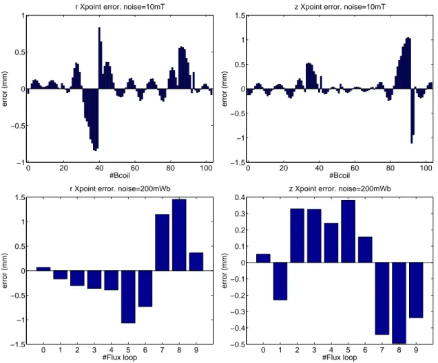
Finally in order to get some insight of the impact of a noisy sensor on the reconstruction of the X point position with the TH algorithm we have conducted 104+10
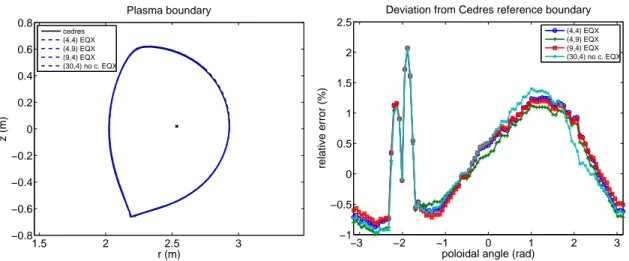
1.5 2 2.5 3 −0.8 −0.6 −0.4 −0.2 0 0.2 0.4 0.6 0.8 r (m) z (m) Plasma boundary cedres (4,4) EQX (4,9) EQX (9,4) EQX (30,4) no c. EQX −3 −2 −1 0 1 2 3 −1 −0.5 0 0.5 1 1.5 2 2.5
poloidal angle (rad)
relative error (%)
Deviation from Cedres reference boundary
(4,4) EQX (4,9) EQX (9,4) EQX (30,4) no c. EQX
Figure 6. Left: Plasma boundaries. Boundaries computed by Equinox (EQX) with (ne = 4, ni = 4) or (ne = 9, ni = 4) and (ne = 30, ni = 4) without any PF coils modelization (no c.) are almost superimposed with the reference boundary computed with Cedres++. The boundary computed with Equinox (ne = 4, ni = 9) does not show any irregularities.
Right: Corresponding relative deviation from Cedres++ boundary,
100(ρ − ρCedres)/ρCedresas a function of the poloidal angle θ. The center of the polar coordinate system (ρ, θ) is the magnetic axis from Cedres++ (shown on left figure).
(ne, ni) (4, 4) (4, 9) (9, 4) (30, 4) no c.
||XptT H− XptCedres|| [mm] 6.7 8.6 7.4 7.8
||XptEQX− XptCedres|| [mm] 5.4 5.4 5.4 5.4
||CT H− MagCedres|| [mm] 18.5 18.3 18.5 19.3
||MagEQX− MagCedres|| [mm] 4.4 3.6 4.5 4.0
Table 2. Rows 1 and 2: distance between the X-point given by Cedres and the one computed by the Toroidal Harmonics algorithm (TH) or the one re-computed by Equinox (EQX). Row 3: distance between the current center used as the pole of the toroidal coordinate system in TH and the magnetic axis given by Cedres. Row 4: distance between the magnetic axis given by Cedres and computed by Equinox.
numerical reconstructions each time applying an offset on a different sensor. The results are displayed on Figure 7. Adding an offset of 10 mT on a Bcoil or of 200 mWb on a flux loop pertubates the X-point position of about maximum 1 mm. Again naturally the Xpoint position is more dependent on sensors that are in the divertor region than on others.
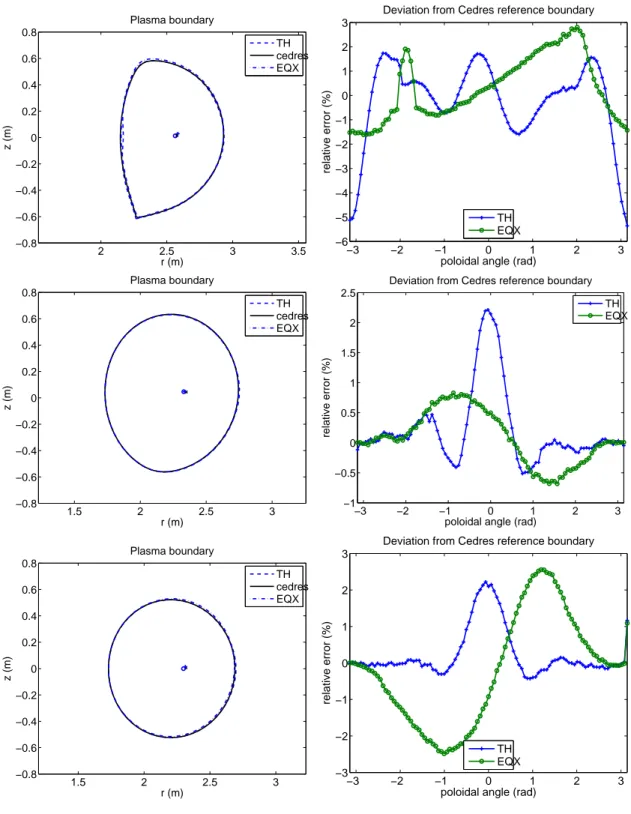
The numerical results for case 2 (smaller plasma) are very similar to those presented above for case 1. It should be mentioned however that the plasma boundary
reconstructed by the TH algorithm with the default (ne = 4, ni = 4) choice presents a
small concavity on the high field side. Nevertheless it is small (distance of maximum 2 cm from Cedres boundary) and again disappears in the plasma boundary computed by Equinox (see Figure 8). In cases 3 and 4 with a limiter configuration the plasma
0 20 40 60 80 100 −1 −0.5 0 0.5 1 #Bcoil error (mm)
r Xpoint error. noise=10mT
0 20 40 60 80 100 −1.5 −1 −0.5 0 0.5 1 1.5 #Bcoil error (mm)
z Xpoint error. noise=10mT
0 1 2 3 4 5 6 7 8 9 −1.5 −1 −0.5 0 0.5 1 1.5 #Flux loop error (mm)
r Xpoint error. noise=200mWb
0 1 2 3 4 5 6 7 8 9 −0.5 −0.4 −0.3 −0.2 −0.1 0 0.1 0.2 0.3 0.4 #Flux loop error (mm)
z Xpoint error. noise=200mWb
Figure 7. Error introduced on X-point position reconstruction by adding a 10 mT offset on a single Bcoil measurement or a 200 mWb offset on a single flux loop measurement.
boundary reconstructions are accurate (see Figure 8). 5.2. Computing time
In view of the possible use of this method for the real time control of the plasma position and shape in the WEST tokamak it is important to evaluate the computing time for one boundary reconstruction. Each evaluation of the flux or the field at a given point has a cost in terms of computing time because the evaluation of the toroidal harmonics as well as the elliptic integrals involved in the expression of the flux generated by a filament of current have one. Therefore in order to have an efficient code, all these functions are precomputed and stored in tables. The evaluation of a function then just involves a linear interpolation between two entries of a table. A second point concerns parallelism. Many loops in the code (matrix assembly, integrals computations, boundary points computation, . . . ) can be parallelized. We have used OpenMP to do so. The program is tested on a Laptop with 2 quadcore processors running at 2.4 GHz. With
this material configuration the code takes about 2 ms for one boundary reconstruction as shown in Table 3. Although this is already in the range of computing time needed for the real time control of the plasma on WEST this result could still be improved using more threads or even GPU as proposed in [30]
Nbr of bnd pts 1 10 20 30 60
Comp. Time (ms) 1.09 1.23 1.44 1.54 1.98
Table 3. Wall clock computing time. 1 boundary point corresponds to the following operations: update of the normal equation matrix as the pole of the toroidal coordinate system changes, solve the normal equation, compute the new current center (to be given to the next time step), compute the point defining the boundary isoflux value ψb (either limiter point or X point). Then add to this the computation of 9, 19, 29 or 59 boundary points for the next columns.
5.3. Equinox on the ITM platform
The method presented in this paper has also been tested on data provided in the ITM database. The aim is to be able to run the equilibrium reconstruction code Equinox directly from the discrete magnetic measurements.
During a first initialization phase all the geometric inputs are read from the database: limiter contour, PFcoils geometry and location, the Bprobes orientation and location, flux and saddle loops location. The convex hull of the limiter contour is computed. This is the Γ contour which is the boundary of the computation domain for the finite element part of Equinox. From this contour a mesh is generated. Of course many other contours could be used as boundary and if desired one can define their own one point by point. However the convex hull of the limiter has the advantage of being computed automatically.
Then comes the time stepping. Each time step is made of two stages. In the first one at the discrete time tn the pole of the toroidal coordinate system is set to the
magnetic axis location computed at time tn−1. The contribution of the different PF
coils to the flux is computed and substracted from the magnetic measurements. The residuals are then fitted to a truncated series of toroidal harmonics.
Once this is done the flux can be evaluated at any point of an unknown annular domain surrounding the plasma and therefore clearly on the contour Γ. We are thus able to compute Cauchy boundary conditions on Γ. Note that even if it is possible in principle we do not compute the plasma boundary at this stage. Indeed we want to run the finite element method of Equinox on a fixed domain which does not need to be re-meshed at each time step. The plasma boundary is thus computed during this second stage as well as all the parameters which characterize a plasma equilibrium (among which the magnetic axis which will be used at the next time step) which are then copied to the ITM database.
6. Conclusion
We have presented in this paper a method based on the use of toroidal harmonics and on a modelization of the poloidal field coils and divertor coils for the 2D interpolation of discrete magnetic measurements.
The method completely relies on the classical assumptions that the equilibrium is axisymmetric and that a negligeable amount of the total current density flows in the plasma existing in the region of the sensors (i.e ∆∗
ψ = 0 holds in this region). If the
first assumption was to be defaulted with non-negligeable 3D effects [31, 32, 33, 34, 35] the method might be destabilized. The same conclusion holds if the second assumption was to fail since the decomposition of the flux in a series of toroidal harmonics with constant coefficients is not exact anymore.
However under these assumptions our numerical results show that the method is quite stable even though it does not involve a classical regularization procedure. This is due to the fact that the ill-posed part of the method that is to say the computation of the internal solution only relies on the choice of the pole of the toroidal coordinate system and on the number of internal toroidal harmonics used to approximate the flux. Our numerical experiments show that the magnetic axis is a good and easy to compute choice for the first point, and concerning the second point that only a few toroidal harmonics are needed to accurately approximate the flux.
The method is generic and can be used to provide Cauchy boundary conditions needed as input by a fixed domain equilibrium reconstruction code like Equinox. This is implemented in the ITM version of Equinox. The method can also be used to extrapolate the magnetic measurements to compute the X-point position and the plasma boundary. It is foreseen to be used in the real time plasma control loop on the WEST tokamak. Acknowledgments
We would like to thank the two anonymous reviewers for their constructive criticism from which the paper has benefitted significantly.
2 2.5 3 3.5 −0.8 −0.6 −0.4 −0.2 0 0.2 0.4 0.6 0.8 r (m) z (m) Plasma boundary TH cedres EQX −3 −2 −1 0 1 2 3 −6 −5 −4 −3 −2 −1 0 1 2 3
poloidal angle (rad)
relative error (%)
Deviation from Cedres reference boundary
TH EQX 1.5 2 2.5 3 −0.8 −0.6 −0.4 −0.2 0 0.2 0.4 0.6 0.8 r (m) z (m) Plasma boundary TH cedres EQX −3 −2 −1 0 1 2 3 −1 −0.5 0 0.5 1 1.5 2 2.5
poloidal angle (rad)
relative error (%)
Deviation from Cedres reference boundary TH EQX 1.5 2 2.5 3 −0.8 −0.6 −0.4 −0.2 0 0.2 0.4 0.6 0.8 r (m) z (m) Plasma boundary TH cedres EQX −3 −2 −1 0 1 2 3 −3 −2 −1 0 1 2 3
poloidal angle (rad)
relative error (%)
Deviation from Cedres reference boundary
TH EQX
Figure 8. Row 1: Case 2
Left : Cedres++ reference and boundaries reconstructed with toroidal harmonics (TH) and Equinox (EQX). Cedres++ and Equinox magnetic axis as well as the computed plasma center taken as the pole of the toroidal coordinate system (circle) are also shown.
Right: Corresponding relative deviation from Cedres++ boundary,
100(ρ − ρCedres)/ρCedresas a function of the poloidal angle θ. The center of the polar coordinate system (ρ, θ) is the magnetic axis from Cedres++ (shown on left figure). Row 2 : same for Case 3. Row 3 : same for Case 4.
[1] J. Blum, C. Boulbe, and B. Faugeras. Reconstruction of the equilibrium of the plasma in a tokamak and identification of the current density profile in real time. J. Comp. Phys., 231:960–980, 2012. [2] Bucalossi J. et al. Feasibility study of an actively cooled tungsten divertor in Tore Supra for ITER
technology testing. Fus. Engin. Des., 86(6-8):684–688, 2011.
[3] J. Wesson. Tokamaks, volume 118 of International Series of Monographs on Physics. Oxford University Press Inc., New York, Third Edition, 2004.
[4] O’Brien D.P., Lao L.L., Solano E.R., Garribba M., Taylor T.S., Cordey J.G., and Ellis J.J. Equilibrium analysis of iron core tokamaks using a full domain method. Nuclear Fusion, 32(8):1351–1360, 1992.
[5] J. Blum. Numerical Simulation and Optimal Control in Plasma Physics with Applications to Tokamaks. Series in Modern Applied Mathematics. Wiley Gauthier-Villars, Paris, 1989. [6] B. Faugeras, A. Ben Abda, J. Blum, and C. Boulbe. Minimization of an energy error functional
to solve a cauchy problem arising in plasma physics: the reconstruction of the magnetic flux in the vacuum surrounding the plasma in a tokamak. ARIMA, 15:37–60, 2012.
[7] D.P. O’Brien, J.J Ellis, and J. Lingertat. Local expansion method for fast plasma boundary identification in JET. Nuclear Fusion, 33(3):467–474, 1993.
[8] F. Sartori, A. Cenedese, and F. Milani. JET real-time object-oriented code for plasma boundary reconstruction. Fus. Engin. Des., 66-68:735–739, 2003.
[9] F. Saint-Laurent and G. Martin. Real time determination and control of the plasma localisation and internal inductance in Tore Supra. Fusion Engineering and Design, 56-57:761–765, 2001. [10] Integrated tokamak modelling. http://portal.efda-itm.eu/, 2013.
[11] B.J. Braams. The interpretation of tokamak magnetic diagnostics. Plasma Phys. Control. Fusion, 33(7):715–748, 1991.
[12] Fock V.A. Fiz. Zh Sovietunion, 1:215, 1932.
[13] Morse P.M. and Feshbach H. Methods of theoritical physics. Cambridge University press, 1953. [14] Lee D.K. and Peng Y.-K. M. An approach to rapid plasma shape diagnostics in tokamaks.
J. Plasma Phys., 25:161–173, 1981.
[15] Deshko G.N., Kilovataya T.G., Kuznetsov Y.K., Pyatov V.N., and Yasin I.V. Determination of the plasma column shape in a tokamak from magnetic measurements. Nuclear Fusion, 23(10):1309– 1317, 1983.
[16] Bondarenko S.P., Golant V.E., Gryaznevich M.P., Kuznetsov Y.K., Pyatov V.N., Taran V.S., Shakhovets K.G., and Yasin I.V. Measurement of the shape of the plasma column in the tuman-3 tokamak. Sov. J. Plasma Phys., 10:520–524, 1984.
[17] Alladio F. and Crisanti F. Analysis of mhd equilibria by toroidal multipolar expansions. Nuclear Fusion, 26(9):1143–1163, 1986.
[18] Van Milligen B.P. Exact relations between multipole moments of the flux and moments of the toroidal current density in tokamaks. Nuclear Fusion, 30(1):157–160, 1990.
[19] Kurihara K. Improvement of tokamak plasma shape identification with a legendre-fourier expansion of the vacuum poloidal flux function. Fusion Tech., 22:334–349, 1992.
[20] Van Milligen B.P. and Lopez Fraguas A. Expansion of vacuum magnetic fields in toroidal harmonics. Comput. Phys. Comm., 81:74–90, 1994.
[21] Y. Fischer. Identification de param`etres magn´etiques `a l’int´erieur d’un tokamak. Journal europ´een des syst`emes automatis´es, 46(6-7):611–632, 2012.
[22] N.N. Lebedev. Special Functions and their Applications. Dover Publications, 1972.
[23] B.J. Braams. Computational studies in Tokamak equilibrium and transport. PhD thesis, University of Utrecht, 1986.
[24] Y. Fischer. Approximation dans des classes de fonctions analytiques g´en´eralis´ees et r´esolution de probl`emes inverses pour les tokamaks. PhD thesis, Universit´e de Nice-Sophia Antipolis, 2011. [25] M. Abramowitz and Stegun I.A. Handbook of Mathematical Functions. National bureau of
Standards, Washington, DC, 1964.
[27] Segura J. and Gil A. Evaluation of toroidal harmonics. Comput. Phys. Comm., 124:104–122, 2000.
[28] L.E Zakharov and V.D. Shafranov. Equilibrium of a Toroidal Plasma with Non-circular Cross Section. Sov. Phys. Tech. Phys., 18:151–156, 1973.
[29] P. Hertout, C. Boulbe, E. Nardon, J. Blum, S. Br´emond, J. Bucalossi, B. Faugeras, V. Grandgirard, and P. Moreau. The CEDRES++ equilibrium code and its application to ITER, JT-60SA and Tore Supra. Fusion Engineering and Design, 86(6):1045–1048, 2011.
[30] X N Yue, B J Xiao, Z P Luo, and Y Guo. Fast equilibrium reconstruction for tokamak discharge control based on GPU. Plasma Phys. Control. Fusion, 55:9pp, 2013.
[31] W. A. Cooper, J. P. Graves, and O. Sauter. Helical ITER hybrid scenario equilibria. Plasma Phys. Control. Fusion, 53:024002, 2011.
[32] W. A. Cooper et al. Bifurcated helical core equilibrium states in tokamaks. Nuclear Fusion, 53:073021, 2013.
[33] S. Lazerson and I. T. Chapman. STELLOPT modeling of the 3D diagnostic response in ITER. Plasma Phys. Control. Fusion, 55:084004, 2013.
[34] J. D. Hanson et al. Non-axisymmetric equilibrium reconstruction for stellarators, reversed field pinches and tokamaks. Nuclear Fusion, 53:083016, 2013.
[35] A.D. Turnbull et al. Comparisons of linear and nonlinear plasma response models for non-axisymmetric perturbations. Phys. Plasmas, 20:056114, 2013.