HAL Id: hal-00317153
https://hal.archives-ouvertes.fr/hal-00317153
Submitted on 1 Jan 2003
HAL is a multi-disciplinary open access
archive for the deposit and dissemination of
sci-entific research documents, whether they are
pub-lished or not. The documents may come from
teaching and research institutions in France or
abroad, or from public or private research centers.
L’archive ouverte pluridisciplinaire HAL, est
destinée au dépôt et à la diffusion de documents
scientifiques de niveau recherche, publiés ou non,
émanant des établissements d’enseignement et de
recherche français ou étrangers, des laboratoires
publics ou privés.
Combining global and multi-scale features in a
description of the solar wind-magnetosphere coupling
A. Y. Ukhorskiy, M. I. Sitnov, A. S. Sharma, K. Papadopoulos
To cite this version:
A. Y. Ukhorskiy, M. I. Sitnov, A. S. Sharma, K. Papadopoulos. Combining global and multi-scale
features in a description of the solar wind-magnetosphere coupling. Annales Geophysicae, European
Geosciences Union, 2003, 21 (9), pp.1913-1929. �hal-00317153�
Annales
Geophysicae
Combining global and multi-scale features in a description of the
solar wind-magnetosphere coupling
A. Y. Ukhorskiy1, M. I. Sitnov2, A. S. Sharma2, and K. Papadopoulos1,2
1Department of Physics, University of Maryland at College Park, USA 2Department of Astronomy, University of Maryland at College Park, USA
Received: 5 November 2002 – Revised: 30 May 2003 – Accepted: 9 June 2003
Abstract. The solar wind-magnetosphere coupling during substorms exhibits dynamical features in a wide range of spa-tial and temporal scales. The goal of our work is to combine the global and multi-scale description of magnetospheric dy-namics in a unified data-derived model. For this purpose we use deterministic methods of nonlinear dynamics, together with a probabilistic approach of statistical physics. In this paper we discuss the mathematical aspects of such a com-bined analysis. In particular we introduce a new method of embedding analysis based on the notion of a mean-field di-mension. For a given level of averaging in the system the mean-filed dimension determines the minimum dimension of the embedding space in which the averaged dynamical sys-tem approximates the actual dynamics with the given accu-racy. This new technique is first tested on a number of well-known autonomous and open dynamical systems with and without noise contamination. Then, the dimension analysis is carried out for the correlated solar wind-magnetosphere database using vBS time series as the input and AL index as
the output of the system. It is found that the minimum em-bedding dimension of vBS−ALtime series is a function of
the level of ensemble averaging and the specified accuracy of the method. To extract the global component from the ob-served time series the ensemble averaging is carried out over the range of scales populated by a high dimensional multi-scale constituent. The wider the range of multi-scales which are smoothed away, the smaller the mean-field dimension of the system. The method also yields a probability density func-tion in the reconstructed phase space which provides the ba-sis for the probabilistic modeling of the multi-scale dynam-ical features, and is also used to visualize the global por-tion of the solar wind-magnetosphere coupling. The struc-ture of its input-output phase portrait reveals the existence of two energy levels in the system with non-equilibrium dy-namical features such as hysteresis which are typical for non-equilibrium phase transitions. Further improvements in space weather forecasting tools may be achieved by a combi-Correspondence to: A. Y. Ukhorskiy ([email protected])
nation of the dynamical description for the global component and a statistical approach for the multi-scale component. Key words. Magnetospheric physics (solar wind– magnetosphere interactions; storms and substorms) – Space plasma physics (nonlinear phenomena)
1 Introduction
The magnetospheric dynamics during substorms exhibits both globally coherent and multi-scale features. The globally coherent behavior of the magnetosphere is evident in such large-scale phenomena as the formation and ejection of plas-moids, the recovery of the field lines from the stretched to a more dipole-like configuration, the formation of global cur-rent systems, etc. At the same time, a number of small-scale phenomena observed during substorms, such as MHD turbu-lence, bursty bulk flows, current disruption, etc., are multi-scale in nature; viz. they have broad band power spectra in a wide range of spatial and temporal scales. The traditional approach of modeling the magnetospheric dynamics is the first principal approach which explicitly takes into account the nature of all forces in the system and then derives its col-lective behavior by considering interactions on the scales de-termined by the model. However, it is well recognized now that the collective behavior of a large number of complex many-body systems is determined by only generic dynamical features such as the range of interaction forces, dimension-ality, and the nature of the order parameter. The dynamical models of such systems can be derived directly from data us-ing general principals of nonlinear dynamics and statistical physics. The clear advantage of such data-derived models is their ability to reveal inherent features of dynamics, even in the presence of complexity and strong nonlinearity. More-over, in many cases they still yield more accurate results and require much less computational power than the first princi-pal models.
1914 A. Y. Ukhorskiy et al.: Global and multi-scale features of magnetospheric dynamics The earlier dynamical models of magnetospheric activity
were motivated by the global coherence indicated by the ge-omagnetic indices and inspired by the concept of dynamical chaos. They were based on the assumption that the multi-scale spectra of observed time series are mainly attributed to the nonlinear dynamics of a few dominant degrees of free-dom (see reviews: Sharma, 1995; Klimas et al., 1996). The dimension analyses of AE time series gave evidence of low effective dimension in the system (Vassiliadis et al., 1990; Sharma et al., 1993). Further elaboration of this hypothe-sis resulted in creating space weather forecasting tools based on local-linear filters (Price et al., 1994; Vassiliadis et al., 1995; Valdivia et al., 1996), data-derived analogues (Klimas et al., 1997; Horton et al., 1999), and neural networks (Her-nandes et al., 1993; Gleisner and Lundstedt, 1997; Weigel et al., 2002). The low dimensional organized behavior of the magnetosphere on global scales is also evident in many in situ observations of the large-scale features of substorms by many spacecrafts including INTERBALL and GEOTAIL missions (Petrukovich et al., 1998; Nagai et al., 1998; Ieda et al., 1998).
However, the subsequent studies have shown that not all aspects of magnetospheric dynamics during substorms con-form to the hypothesis of low dimensionality and thus cannot be accounted for within the framework of dynamical chaos and self-organization. For example, the power spectrum of
AE index data (Tsurutani et al., 1990) and magnetic field fluctuations in the tail current sheet (Ohtani et al., 1995) have a power-law form typical for high dimensional colored noise. Prichard and Price (1992) have argued that by using a mod-ified correlation integral (Theiler, 1991), a low correlation dimension cannot be found for the magnetospheric dynam-ics. Moreover, detailed analyses (Takalo et al., 1993, 1994) have shown that the qualitative properties of AE time se-ries are much more similar to the bicolored noise than to the time series generated by a low dimensional chaotic system. It was also shown (Ukhorskiy et al., 2002a) that the low di-mensional dynamical models leave out a significant portion of the observed time series which is associated with high di-mensional multi-scale dynamical constituent.
One interpretation of these multi-scale aspects of magne-tospheric dynamics was a multifractal behavior generated by intermittent turbulence (Borovsky et al., 1997; Consolini et al., 1996; Angelopoulos et al., 1999). Another approach to magnetosphere modeling is based on the concept of self-organized criticality (SOC). SOC was first introduced by Bak et al. (1987), who claimed that in “sand-pile” cellular automata the “criticality” (power distribution of avalanches which conduct the energy transport in the system) arises spontaneously without tuning of the control parameters. In SOC models the multi-scale features of substorms were re-produced by a “sand-pile” or other non-equilibrium cellular automata which explicitly take into account the large num-ber of degrees of freedom in the system and the interactions among them on different scales (Consolini, 1997; Uritsky and Pudovkin, 1998; Watkins et al., 1999, 2001; Takalo et al., 1999; Chapman and Watkins, 2001; Uritsky et al., 2002).
However, it was shown (Vespignani and Zapperi, 1998) that in order for the system to achieve criticality, the fine tuning of control parameters is required. In the cellular automata models, like “sand-pile” or “forest fire” models, the fine tun-ing corresponds to the vanishtun-ing values of input parameters. This makes these systems effectively autonomous and thus questions the relevance of the SOC framework to the mag-netosphere, whose dynamics is, to a large extent, driven by the solar wind input. Moreover, original SOC models gener-ally cannot account for the large-scale coherent features of the magnetosphere, since in most SOC models the multi-scale properties of the system are essentially independent of the global dynamics. To reconcile the multi-scale fea-tures with the global dynamics in a SOC-like model, the “sand-pile” model with the modified dynamical rules was proposed (Chapman, 2000; Chapman et al., 2001). In this model the scale-invariant avalanches were found to coexist with system-wide large-scale events. However, since such system-wide avalanches were found only in the “sand-pile” models with a vanishing rate of the energy input, this still cannot account for the specific global features of the actual magnetospheric dynamics. The SOC concept generalized for continuous systems (Lu, 1995) was further elaborated in the MHD model of the magnetospheric plasma sheet driven by a noise-like input (Klimas et al., 2000). However, the SOC regime in this model was achieved by assuming the spe-cific form of the time dependence of the diffusion coefficient, whose relevance to the real magnetospheric plasma sheet is still an open question. On the other hand, it was also noted (Chang, 1999, 2000) that the properties of the criticality in SOC and in forced SOC models are very similar to those of the critical point in phase transitions.
In the physics of phase transitions, it is well known that the multi-scale behavior can naturally coexist with global dy-namics. There are two different types of phase transitions which are intimately related to each other and coexist in a sin-gle system. The global dynamics of the system corresponds to the low dimensional manifold (coexistence surface) in the phase space of the system, which separates different phases of matter like the “pressure-temperature-density” surface in the case of a liquid-gas system. Due to the slow changes in the control parameters the state of the system evolves along the coexistence surface to the point where its stability is lost and it jumps to the state with lower energy through the first order phase transition. In first-order phase transitions one or more of the first derivatives of the appropriate thermody-namic potential (e.g. free energy) are discontinuous. The singular point of the coexistence surfaces where the order parameter (e.g. density in liquid-gas transitions, magneti-zation in ferromagnets) vanishes corresponds to the second order phase transitions and is called the critical point. At the critical point the first derivative of the thermodynamic poten-tial is continuous while the second order derivative breaks. The approach to the critical point corresponds to an increase in fluctuations of the control parameter. At the critical point the fluctuations are scale-invariant and the correlation length (the size of the maximum fluctuation) diverges according to
the power law. It is worth noting that the fluctuation growth is not restricted only to the critical point vicinity. Indeed, the order parameter can exhibit fluctuations in a wide range of scales during the first order phase transitions as well, such as the growth of steam bubbles in boiling water. The more fun-damental difference between the first and second order phase transitions is that during the former, the symmetry in the sys-tem is preserved, while during the later the symmetry breaks down (Stanley, 1971; Landau and Lifshitz, 1976). Phase transitions in natural, non-autonomous systems are essen-tially dynamic and non-equilibrium, resulting in additional properties such as hysteresis and dynamical critical expo-nents (Charkrabarti and Acharyya, 1999; Zeng et al., 1999; Hohenberg and Halperin, 1977).
The magnetospheric dynamics during substorms shares a number of properties with the dynamic non-equilibrium phase transitions (Sitnov et al., 2000; Sharma et al., 2001; Sitnov et al., 2001). In particular, using the global singular spectrum analysis of vBS−ALdata Sitnov et al. (2000) have
shown that the global magnetospheric dynamics is organized in a manner similar to the “pressure-temperature-density” di-agram of the water-steam system. It was also suggested that the multi-scale properties of the data can be attributed to the dynamics in the critical point vicinity, i.e. second order phase transitions. Sitnov et al. (2001) also established the relation between the magnitude of the largest fluctuations of AL time derivative and the solar wind parameters similar to the input-output critical exponent β. The phase transition-like behav-ior was also found in other substorm signatures. In particu-lar, it has been noted (Consolini and Lui, 1999) that the cur-rent disruption is similar to the second order phase transition. Consolini and Michelis (2001) proposed the cellular automa-tion model of solar wind-magnetosphere coupling based on a revised forest-fire model (Drossel and Schwabl, 1992). The model has a repulsive fixed point similar to the critical point in phase transitions. The model was driven by the chaotic time series with the spectral properties of solar wind. It was found that the power spectrum of the integrated output has the broken power-law shape similar to the AE index spec-trum and that the relaxation phenomena occurred as sporadic localized events similar to BBF.
The phase transition analogy clearly provides a framework for understanding the magnetospheric dynamics in which the global and multi-scale processes coexist. This also led to a new approach to the data-derived modeling of the solar wind-magnetosphere coupling that combines the methods of nonlinear dynamics and statistical physics (Ukhorskiy et al., 2002b). In the present paper we discuss the mathematical aspects of such a combined analysis. One of the central con-cepts of this analysis is the notion of mean-field dimension. For the given level of averaging in the system (the number of points in the phase space involved in the averaging) the mean-field dimension determines the minimum dimension of the embedding space in which the averaged dynamical sys-tem approximates the actual dynamics with the given accu-racy (noise level). This also yields the distribution function in the reconstructed phase space which provides the basis
for the probabilistic modeling of the multi-scale dynamical constituent. Previous analysis (Ukhorskiy et al., 2002a) has shown that dynamical models are very similar to the mean-field approach in phase transitions, since their outputs are ob-tained by averaging over the chosen range of scales in the re-constructed input-output phase space. Thus, the multi-scale features of the time series not captured by the low dimen-sional models are essentially the deviations of the data from the mean-field model. According to the phase transition anal-ogy, the magnitudes of these fluctuations may be related to the solar wind input in a probabilistic fashion similar to the input-output critical exponent. The question is to what ex-tent the magnetosphere can be described as a deterministic system and at what point the probabilistic consideration is necessary. In this paper we address this question with the use of the delay embedding analysis of a vBS−ALtime series.
We introduce a new technique of estimating the minimum embedding dimensions of input-output dynamical systems in the presence of a stochastic component.
It is now recognized that if all interaction scales are taken into account, the magnetosphere cannot be considered as a low dimensional system. However, introducing the proba-bility density function on the attractor and performing the ensemble averaging in the embedding space leads to the smoothing of the small-scale high dimensional component. Such averaged system has a finite dimension and thus allows for a deterministic description. The dynamical model built into the embedding space of the averaged system yields the regular component of the observed time series. The portion of the time series not captured by the low dimensional model corresponds to the high dimensional constituent, which is smoothed away after the ensemble averaging and may be treated as noise from the dynamical modeling point of view. It is also found that the delay embedding of the time series containing a high dimensional constituent is not unique in the sense that there is a continuum of ways of extracting the coherent portion from the observed time series. A particular choice of the embedding parameters sets the complexity of the resultant dynamical model, viz. the dimension of the em-bedding space, and the permissible noise level. The higher the complexity is, the smaller the noise level in the system, but the larger the amount of data and thus the greater the com-puting power needed for constructing the dynamical model of the system. In addition to the embedding space parame-ters, the new technique presented in this paper also yields an estimation of the probability density function in the recon-structed phase space. Its moments yield the average dynam-ical properties of the system, while its evolution with input parameters gives a full description of the collective behavior in the system. Thus, it can be used to model and forecast the high dimensional portion of the observed dynamics not predicted by low dimensional deterministic models.
The next section discusses the methods of determining the minimum embedding dimensions and the necessity of intro-ducing a new method in the case of the time series with a high dimensional component or noise. Then, we describe the method and its applications to different dynamical systems.
1916 A. Y. Ukhorskiy et al.: Global and multi-scale features of magnetospheric dynamics
Unknown
System
Output
Input
O(t)
I(t)
Fig. 1. Structure of an input-output system.
In Sect. 3 the embedding analyses of the AL − vBStime
se-ries are presented and the application of the probability den-sity function to the study of the global constituent in the solar wind-magnetosphere coupling is discussed. The last section presents the main results of the paper and their implications to magnetospheric modeling.
2 Estimating the embedding dimension
A large portion of the magnetospheric dynamics is driven by the solar wind input. Therefore, the method of estimating the minimum embedding dimensions of the vBS−ALtime
series should be valid for non-autonomous systems. More-over, the examination of the multi-scale properties of the so-lar wind-magnetosphere coupling showed (Ukhorskiy et al., 2002a) that the multi-scale constituent of the AL time se-ries has dynamical and statistical properties similar to those of the colored noise. One of the possible origins of this multi-scale portion of AL is the scale-invariant constituent of its driver, vBS (Freeman et al., 2000; Hnat et al., 2002).
Thus, it is required that the method is also valid for the ran-dom systems, where dynamics is driven by a ranran-dom process (Arnold, 1998).
There has been much work on determining the embedding dimensions of the time series generated by autonomous dy-namical systems in the absence of dydy-namical noise (see re-view: Abarbanel et al., 1993). The methods developed for estimating the minimum embedding dimension are grounded on Takens’ embedding theorem (Takens, 1981; Sauer et al., 1991), and most of them use the ideas of the false nearest neighbors technique (Kennel et al., 1992; Cao, 1997). Later, a number of works discussed the theoretical foundations of the delay embedding of the input-output time series (Cas-dagli, 1993; Stark et al., 1996). This led to the generaliza-tions of the existing method for the case of non-autonomous dynamical systems (Rhodes and Morari, 1997; Cao et al., 1998). Recently, considerable attention was drawn to the em-bedding analyses of the time series generated by random dy-namical systems (Muldoon et al., 1998; Stark, 2001). How-ever, these methods are not applicable to the magnetospheric time series analysis, since they generally cannot distinguish between the pure noise and a low dimensional time series with noise contamination. Thus, for estimating the embed-ding dimension of the vBS−ALtime series a new approach
is required. In the following we discuss a new method for es-timating the delay embedding parameters of random dynam-ical systems. The method is applicable to both autonomous and open systems, and therefore, for the sake of
general-ity, the description will be given for the case of the input-output time series. In the case of a noise-free dynamical sys-tem, whose evolution is given by a finite set of coupled ordi-nary differential equations, the observed time series data is a function only of the state of the underlying system and con-tains all the information necessary to determine its evolution. Thus, if a space large enough to unfold the dynamical attrac-tor is reconstructed from the time series and the present state of the system is identified, then the dynamics of the system can be inferred from the known evolution of similar states. The phase space can be reconstructed by a delay embedding method which provides the unique correspondence between the original dynamics and the dynamics in the embedding space. The embedding theorem (Takens, 1981) states that in the absence of noise, if M ≥ 2N +1, then M-dimensional de-lay vectors generically form an embedding of the underlying phase space of the N -dimensional dynamical system. In the case of non-autonomous systems (Fig. 1) the M-dimensional embedding space is formed by the input-output delay vec-tors:
(ITt ,OTt ) =
(It, It −1, ..., It −(MI−1), Ot, Ot −1, ..., Ot −(MO−1)), (1) where It =I (t ), Ot =O(t ), M = MI +MO. If the delay
matrix A is defined as:
A = IT0,OT0 . . . ITN t,OTN t (2) C = ATA; Cvk =w2kvk ∈RM, k =1, ..., M, (3)
then C is the covariance matrix. Since C is Hermitian by definition, its eigenvectors {vk} form an orthonormal basis
in the embedding space. Vectors {vk}, which are referred to
as principal components, are usually calculated by using the singular value decomposition (SVD) method, according to which any M × Ntmatrix A can be decomposed as:
A = U · W · VT = r X k=1 wk·uk⊗vk, (4) where V = (v1, ...,vM),U = (u1, ...,uM), W = diag(w1, ..., wM), w1≤w2≤... ≤ wM U · UT =1, V · VT =1.
The set of all delay vectors forms an irregular cloud in RM. If the number of delays M is greater than the minimum di-mension required for the delay embedding of the observed time series, then there are directions in RM into which this cloud does not extend. In this case the singular spectrum
n
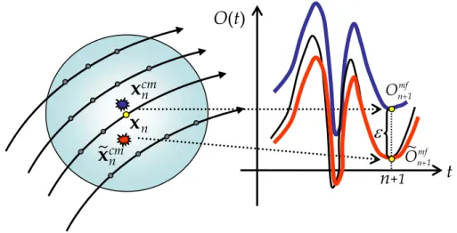
+1t
O(t)
ε
nx
cm nx
cm n~x
mf nO
+1 mf nO
1~
+Fig. 2. Graphical representation of determining the embedding parameters of the observed time series.
analysis helps to find the subspace relevant for constructing the dynamical model of the system (Broomhead and King, 1986). The eigenvalues w2k are the squared lengths of the semi-axes of the hyper-ellipsoid which best fit the cloud of data points and the corresponding eigenvectors, vk, give the
directions of the axes. The most relevant directions in space are thus given by the principal components corresponding to the largest eigenvalues. Therefore, instead of the input-output delay vector (1) in the embedding space, its projection on the first D principal components:
xt =(ITt ,O T
t ) · (v1, ...,vD), (5)
where D is the minimum embedding dimension, yields a bet-ter representation of the system. In this case, if M is substan-tially greater than D, small variations of MI and MOdo not
change the state of the system. For simplicity, all calculations in this paper are performed with MI =MO.
If the embedding procedure is properly performed, that is, if the attractor of the system was completely unfolded, then reconstructed states, xn, have a one-to-one correspondence
with the states in the original phase space and thus can be used for construction of the dynamical model of the system (Farmer and Sidorowich, 1987; Casdagli, 1989, 1993; Sauer, 1993). For this purpose it is assumed that the underlying dy-namics can be described as a nonlinear scalar map (6), which relates the current state to the manifestation of the following state regarding the output time series value at the next time step. The unknown nonlinear function F is approximated locally for each step of the map by the linear filter:
Ot +1=F (xt) ≈ F (˜xt) + αt·δxt, (6)
where ˜xt is the expansion point. Filter coefficients are
cal-culated using the known data, referred to as the training set, which is searched for the states similar to the current, that is, the states that are closest to it, as measured by the dis-tance in the embedding space defined using the Euclidean metric. These states are referred to as nearest neighbors.
Strictly speaking, the choice of the expansion point is some-what arbitrary and may be different for different applications. For chaotic time series forecasting in autonomous dynamical systems Sauer (1993) suggested that better predictability is achieved when the average state vector of N N nearest neigh-bors xk, which is also called the center of mass, is taken as
the center of expansion:
xcmt = 1 N N N N X k=1 xk,xk ∈N N. (7)
It may appear that choosing a particular center of the expan-sion is an auxiliary procedure that leads only to some in-crease in the accuracy of the model. However, it was shown (Ukhorskiy et al., 2002a) that, in the case of the Earth’s magnetosphere, and presumably for a large class of non-autonomous real systems, the expansion about the center of mass may be essential for modeling the system’s dynamics with the use of local-linear filters. It allows for a separa-tion of the regular dynamical constituent, stabilizes the pre-diction algorithm, and provides the basis for modeling the multi-scale dynamical features. It was also shown that, for the purpose of the long-term prediction, the right-hand side of the model (6) can be reduced to its zeroth term, i.e. the arithmetic average of the outputs corresponding to a one step iterated nearest neighbors equation:
Ot +1mf =F (xcm
t ) = hOk+1i,xk∈N N. (8)
As will be shown later, using the center of mass also plays a central role in estimating the minimum embedding dimen-sions of the time series generated by random dynamical sys-tems.
In the case of a low dimensional coupled dynamical sys-tem the minimum embedding dimension of its time series can be easily inferred directly from data by determining the space where all false crossings of the orbits, which arose by virtue of having projected the attractor into a low dimen-sional space, that was too low, disappear. In the original false
1918 A. Y. Ukhorskiy et al.: Global and multi-scale features of magnetospheric dynamics
(a)
(b)
(c)
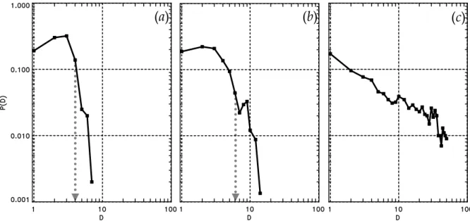
Fig. 3. Distribution functions of Dncalculated with N N = 3 for the time series generated by different autonomous dynamical systems. In
all three cases MI =M + O =50. Grey arrows show possible choices of the embedding space dimension. (a) Lorenz attractor (dt = 0.01). Distribution function rapidly drops to zero at D = 3 − 4. (b) Mackey–Glass delay-differential equation (dt = 0.1). Distribution function drops to zero at D = 6 − 7. (c) 1/f -noise generator. The power shape of the distribution function indicates the absence of finite embedding dimensions.
nearest neighbors method (Kennel et al., 1992), as well as in its generalized versions (Cao, 1997; Rhodes and Morari, 1997; Cao et al., 1998), this is done by examining whether a given state of the system and the state which was identi-fied as its closest neighbor are nearest neighbors by virtue of the projection into a low dimensional space that was too low. The minimum dimension is assessed by examining all points of the attractor in dimension one, then dimension two, etc., until there are no incorrect or false neighbors remain-ing. This approach works well for determining the minimum embedding dimension of the time series generated by a wide class of autonomous and open systems in which dynamics is not subjected to noise. However, this method is not applica-ble to the time series generated by dynamical systems which exhibit randomness.
Let us consider the dynamics of a low dimensional system in the embedding space (assuming that the embedding pro-cedure was performed correctly). In the absence of noise all attractor’s trajectories lie on a smooth manifold. The dynam-ics of the system is coherent and have the same properties on all scales, starting at the largest scale given by the size of the attractor and ending at the smallest scale given by the number of data points in the training set. No two trajecto-ries can intersect in this case, and any two states of the sys-tem can be resolved. Such syssys-tem has a fixed dimension at all scales, defined by the dimension of the space which pro-vides the embedding of the manifold containing the dynam-ical attractor. This picture considerably changes when noise is introduced in the system. The effect of noise is somewhat similar to a diffusion. It destroys the coherence of the dynam-ics on small scales, smearing the attractor points around the
manifold containing “clean” dynamics. Moreover, the delay embedding in its original sense does not exist in this case, since there is no smooth manifold containing the dynamical trajectories in any finite dimension. States of the system ly-ing within the range of scales affected by noise cannot be resolved. Thus, in this case any method similar to the false nearest neighbors, which examines the structure of the attrac-tor on the smallest possible scale, will indicate that the sys-tem is high dimensional and a proper embedding has not been achieved. However, if the small-scale dynamical constituent affected by noise is smoothed away, then the averaged system allows for delay embedding. In random systems the range of scales in the embedding space, affected by noise depends on the noise amplitude, the inherent properties of the system and the embedding space dimension. Thus, embedding of the time series generated by random systems should be consid-ered as a procedure of choosing the embedding space as well as determining the range of scales in this space which has to be smoothed away. In other words, introducing a probability density function on the attractor corresponding to the partic-ular dimension of the embedding space and performing the ensemble averaging yields the smooth manifold which con-tains the coherent portion of the observed time series.
For a time series not contaminated by noise the criterion for a good embedding can be stated as follows. If two states xk and xn, are close in the embedding space, then according
to Eq. (6) the values of a one step iterated scalar time series corresponding to these states, Ok+1and On+1, should also
be close. In the case of random dynamical systems this is not necessarily true, since on small scales the coherence in system’s dynamics might be destroyed by noise. In this
A. Y. Ukhorskiy et al.: Global and multi-scale features of magnetospheric dynamics 1919 case it is essential to not only find the dimension, but also
to determine the range of scales in this space which is populated by high dimensional dynamics and thus needs to be smoothed away. For that we suggest to substitute the above criterion by the following approach. Let us consider two states xn and xk, of the random system in the space
formed by the first D eigenvectors of the covariance matrix
{vk|k = 1, ..., D}, together with the sets of their nearest
neighbors identified with the use of a Euclidean metric in this space. By analogy with the noise-free dynamical systems we consider this space to be an embedding space of the underlying dynamics, if there is an N N such that the following criterion is satisfied for any two states of the system:
if kxcmn −xcmk k→0 then |On+1mf −Ok+1mf | →0, (9) where the center of mass vectors are given by Eq. (7). This condition provides that the function F in Eq. (8) is well de-fined, i.e. xcmk =xcm n whenever O mf k+1=O mf n+1.
According to this definition the embedding procedure con-sists of finding two parameters, D and N N . If such parame-ters are defined, then a dynamical model of the system can be introduced in the form of Eq. (9). Averaging over N N near-est neighbors defines the smooth manifold of dimensionality
Dor smaller that can be fit locally to the data and then used to interpolate the dynamics of the system. As will be shown later for many random systems the choice of D and N N is not unique. In such cases D is usually a decreasing func-tion of N N , the higher the D, the smaller the N N required for the embedding. The particular choice of the embedding parameters should be justified in each particular case by the accuracy of the dynamical model. The higher the N N , the stronger the averaging introduced into the system and thus, a larger portion of the time series is considered to be noise from the dynamical model point of view. However, it turns out that a decrease in N N does not always lead to an increase in the model’s accuracy, and thus, for modeling purposes it is not always preferable to minimize it. Moreover, a decrease of N N in many cases leads to a growth of D which is nec-essary for a good embedding, which increases the amount of data needed and computational power required for construct-ing the model.
For calculation purposes the criterion (9) can also be for-mulated in the following way (see Fig. 2). A D-dimensional space is considered to be an embedding space, if there is a number N N such that for all points n from the data set the inclusion of the state xn in the set of its nearest neighbors
does not considerably change the value of the average of the outputs corresponding to a one step iterated nearest neigh-bors equation. In other words:
kxcmn − ˜xcmn k→0 H⇒ |On+1mf − ˜On+1mf | →0 xcmn = 1 N N N N X k=1 xk, ˜xcmn = 1 N N(xn+ N N −1 X k=1 xk),xk∈N N. (10)
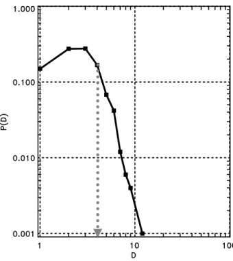
Fig. 4. Distribution functions of Dncalculated with N N = 3 and
MI =MO=50 for the time series generated by the synchronized Lorenz attractor. Distribution function drops rapidly to zero around
D =4.
Thus, for determining the optimal embedding parameters
D and N N the following algorithm is proposed. First, the parameter N N is fixed at some small value. Then, for each point (In, On)of the input-output time series the conditions
of criteria (10) are considered in dimension one, then dimen-sion two, etc., until they are satisfied in some dimendimen-sion Dn.
In other words we seek for:
min Dn: |On+1mf − ˜On+1mf |< ε, (11)
where ε is some small number which sets the precision in the system. Quantities differing by less than ε are consid-ered to be identical within the permissible accuracy. When
Dnis found for all points in the training set, the probability
distribution of Dnis calculated. If the system has a finite
em-bedding dimension for a chosen value of N N , then the dis-tribution function will drop to zero at this value. If there is no finite embedding dimension for this value of N N , the dis-tribution function has a power-law dependence. In this case
N Nis increased and the whole procedure is repeated until a finite dimension is found. Then, for all pairs of parameters (N N, D) the dynamical models (8) are calculated and their outputs are compared. The parameters which yield the high-est accuracy of the model are considered as optimal. The delay embedding of the input-output time series generated by systems with a random component follows from dynam-ical systems theory based on Takens’ embedding theorem. However, this technique of determining the embedding pa-rameters is very similar to the methods known in statistical physics. This recognition can be used as a link between the
1920 A. Y. Ukhorskiy et al.: Global and multi-scale features of magnetospheric dynamics
(a)
(b)
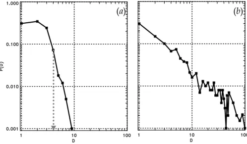
Fig. 5. Distribution functions of Dncalculated with N N = 3 and MI =MO=50 for the time series generated by the synchronized Lorenz
attractor with 1/f -noise contamination. (a) Small noise amplitude (ε = 0.5 > σ1/f =0.4). Distribution function drops rapidly to zero at
D =4. (b) Large noise amplitude (ε = 0.5 σ1/f = 15). The power shape of the distribution function indicates the absence of finite embedding dimensions at the small scales.
deterministic and probabilistic approaches to modeling the collective behavior in random systems. It was pointed out earlier (Ukhorskiy et al., 2002a) that the dynamical model (8) is very similar to the mean-field approach in thermodynamics (e.g. Kadanoff, 2000), since its output is obtained by the av-eraging over the chosen range of scales in the reconstructed phase space. For that the reconstructed D-dimensional space is divided into the equal-probability clusters centered on ev-ery point of the data set. The size of the cluster is defined by the radius R of a sphere containing the set of N N near-est neighbors. This defines the fixed-probability partition of the phase space, which consists of a large number of over-lapping clusters, all containing the same number of points but having different spatial sizes. Thus, after parameters D and N N are found the probability density function of sys-tem states in the embedding space can be estimated using the
K-nearest-neighbor approach (Bishop, 1995):
ρ(x) = A
R(x, N N )D, (12)
where the constant A is defined by the normalization condi-tion. To obtain the model output the average is taken only over the states within a given cluster, while the states outside this cluster are considered to be independent and, therefore, do not contribute to the output. In other words, the output of the mean-field model (8) is calculated by taking the ensemble averaging with the use of the distribution function (12). From this point of view, the method presented here for determin-ing the embedddetermin-ing parameters has another very transparent meaning. It assures that in the reconstructed phase space the ensemble averaging is well defined, viz. the average parame-ters are close to the exact parameparame-ters of the system. This also means that the mean-field approach is valid for the descrip-tion of the collective behavior of the system.
Thus, the presented method can be considered as a tech-nique of determining the mean-field dimensions of random dynamical systems, since it yields the parameters of the mean-field dynamical model, even when the embedding in its original sense does not exist, i.e. the system is high di-mensional at small scales and, therefore, does not allow for the exact deterministic consideration. Before proceed-ing with the mean-field dimension analysis of the magneto-spheric dynamics we test this method on several well-known autonomous and open dynamical systems, with and without noise. As was mention before, the calculations are not sensi-tive to the variations in the number of input and output delays in (1). All embedding analyses in this paper were carried out for MI =M0=50, and the delay time is equal to the
sam-pling time of the time series.
2.1 Autonomous dynamical systems
In this section we determine the embedding dimensions of the time series generated by several autonomous dynamical systems like, Lorenz differential equations, Mackey–Glass delay differential equation, and 1/f -noise generator. 2.1.1 Lorenz attractor
We consider the Lorenz equations (Lorenz, 1963):
˙ x(t ) = σ · (y − x) σ =10 ˙ y(t ) = r · x − y − x · z r =8/3 ˙ z(t ) = −b · z + x · y b =28. (13)
At the given values of parameters the system produces chaotic dynamics. The time evolution in the phase space is organized by two unstable foci and an intervening sad-dle point. The Lorenz attractor is a fractal set lying on the
smooth manifold embedded in three-dimensional Euclidean space. After solving the set (13) with the foorth-order Runge-Kutta, method with integral step 0.01 we apply our method of estimating mean-field dimensions to the x(t ) time series. Since there is no noise in the system, the reconstructed dy-namical attractor should be similar to the original one and thus should have a fixed dimension on all scales. Therefore, the technique is expected to assess the minimum embedding dimension without a significant ensemble averaging. The distribution function of Dnobtained for N N = 3 is shown
in Fig. 3a. It drops to zero rapidly at D values from 3 to 4, and, therefore, according to our method, these D = 3 − 4 are the good choices for the embedding dimensions of a x(t ) time series.
2.1.2 Mackey–Glass equation
As another example of a low dimensional dynamical system we consider the Mackey–Glass delay-differential equation (Mackey and Glass, 1977)
˙
x(t ) = a · x(t − τ )
1 + xc(t − τ )−b · x(t ). (14)
The Mackey-Glass equation is, in principal, infinite-dimensional, in the sense that a future value depends on a continuum of past values. It was shown, however, that for the parameter values of a = 0.2, b = 0.1, c = 10, and
τ =30 the system becomes chaotic with a fractal dimension of about 3.6 (Meyer and Packard, 1992). The equation was solved with the fourth-order Runge-Kutta method, with inte-gral step 0.1. The embedding analyses showed that at these parameter values the dynamical attractor can be embedded in 6-dimensional space (Mead et al., 1992). As in the case of the Lorenz attractor, no averaging is required to determine the minimum embedding dimension. For N N = 3 the Dn
distribution function rapidly drops to zero at D, to about 6–7 (Fig. 3b), and, therefore, good choices for embedding dimen-sion are D = 6 or 7.
2.1.3 1/f -noise
To illustrate what happens if the above analysis is applied to a high dimensional system, we consider the 1/f -noise time se-ries, viz. the time series produced by a random number gen-erator, where the power spectrum drops with an increase in frequency as 1/f . The Dndistribution function calculated for
N N =3 is shown in Fig. 3c. The distribution function has a power dependence on D in the wide range of dimensions (D = 1−100). This indicates that for the given averaging the system does not have a finite mean-field dimension. Since in this case almost no averaging was done (N N = 3), the power shape of the distribution function also means that the observed time series does not allow for the delay embedding in the sense of the original noise-free embedding theorem.
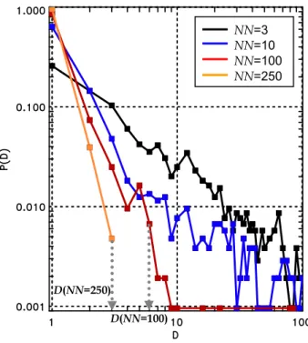
NN=3 NN=50 NN=100 NN=300 D(NN=50) D(NN>100)
Fig. 6. Distribution functions of Dn calculated with ε = 0.5 and
different values of N N for the time series generated by the synchro-nized Lorenz attractor with 1/f -noise contamination (σ1/f). For
different N N the distribution function drops to zero at different val-ues of D. The mean-field dimension decrease with the increase in the range of scale smoothed away after the averaging.
2.2 Input-output time series
Before proceeding with the analysis of noise effects on the delay embedding, we present an example of determining the embedding dimensions of the input-output time series. As an example of a non-autonomous, low dimensional dynamical system we consider a synchronized Lorenz attractor. If the
x(t )component of one Lorenz system is used as a driver for the second Lorenz system, then the attractors of both systems synchronize at the following values of parameters: r = 60,
b = 8/3, σ = 10 (Pecora and Carroll, 1990), i.e. indepen-dent of the initial conditions of the second system; after a few steps its trajectory converges to the attractor of the driver. Thus, the Y (t ) component of the second Lorenz attractor can be considered as an output of the non-autonomous chaotic dynamical system driven by the input –x(t ) component of the first Lorenz attractor. The distribution function of Dn
calculated for N N = 3 is shown in Fig. 4. The rapid drop in the distribution function indicates that D = 3 − 4 are good choices for embedding dimensions of the input-output time series.
2.3 Noise effects
The examples of the time series presented above were gener-ated by low dimensional dynamical systems (except for the 1/f -noise case). Consequently, the mean-field dimensions of
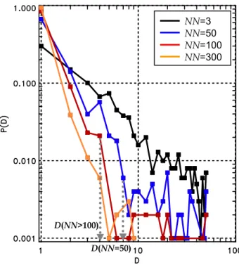
1922 A. Y. Ukhorskiy et al.: Global and multi-scale features of magnetospheric dynamics NN=3 NN=10 NN=100 NN=250 D(NN=100) D(NN=250)
Fig. 7. Distribution functions of Dncalculated with different values
of N N for vBS−ALtime series of Bargatze et al. (1985) database.
For different N N the distribution function drops to zero at different values of D. The mean-field dimension decrease with the increase in the range of scale smoothed away after the averaging.
these systems were determined with almost no averaging and thus do not differ from the minimum embedding dimensions found with the use of other methods, like the false nearest neighbors technique. In this section we consider the effects of noise on the embedding analysis of the observed time se-ries. It is shown that, in the presence of a significant noise component, the delay embedding becomes possible only af-ter averaging the data in the reconstructed phase space. To study the effects of noise on delay embedding we consider the input-output time series of the synchronized Lorenz at-tractor contaminated by a 1/f -noise time series of various amplitudes. The noise amplitude is considered to be small if ε > σ1/f, where σ1/f is the variance of the noise time
series. The distribution function of Dn calculated for the
small noise contamination with N N = 3 is shown in Fig. 5a. As can be seen from the plot the distribution function does not differ much from the distribution function calculated for the clean time series of the synchronized Lorenz attractor (Fig. 4). Since almost no averaging was done, the sharp drop in the distribution function indicates the existence of low di-mensional embedding space (D = 3−4) at the smallest inter-action scales. However, this low dimensional picture signif-icantly changes when the amplitude of the noise is substan-tially increased (ε σ1/f). In this case the Dn distribution
function calculated for N N = 3 has a power shape similar to the distribution function calculated for the 1/f -noise time series (Fig. 5b, Fig. 3c). This means that in the embedding space of any dimension the coherent, low dimensional
dy-namics of the system appears to be destroyed by the noise within some range of scales. Thus, at small scales the dy-namical properties of the systems are indistinguishable from those of the noise itself. This also limits the information that can be extracted by exploring the dynamical trajectories on the smallest scales.
To extract more information about the system’s dynamics and, in particular, to obtain the range of scales affected by noise, we follow the prescription of our method and increase the number of nearest neighbors participating in the averag-ing. Figure 6 shows the Dndistribution functions calculated
for different values of N N . It is seen from the plots that starting at N N = 50 the averaged systems start exhibiting a low dimensional behavior. The particular values of dimen-sions correspond to the minimum embedding dimendimen-sions of the averaged dynamical systems, where the degree of aver-aging is set by N N . The small-scale portion of the time series which is smoothed away due to the averaging is not embedded in this particular dimension. Therefore, the as-sessed dimensions should be considered only as the mean-field dimensions of the system. At N N = 50, D = 7 and for
N N >100, D = 4.
To distinguish the pair of parameters which is optimal for the embedding of the observed time series we use these pa-rameters to build a dynamical model in the form of (8). The optimal parameters are identified as those which provide the highest prediction accuracy of the model. Throughout this paper the prediction accuracy of dynamical models is quan-tified by the normalized mean squared error (N MSE) (Ger-shenfeld and Weigend, 1993)
N MSE = 1 σO v u u t 1 N N X k=1 (Ok− ˆOk)2. (15)
Here, k = 1 to N span the forecasting interval, σO is the
standard deviation of the original output time series, and the
ˆ-symbol denotes the predicted values. The value N MSE = 1 corresponds to a prediction of the average. For (D, N N ) of (7, 50) N MSE = 0.9 and for (4, 100) N MSE = 0.8. Therefore, according to our method the optimal embedding parameters (D, N N ) of the input-output time series gener-ated by the contamingener-ated synchronized Lorenz system are (4, 100).
After the embedding parameters (D, N N ) of the time se-ries are determined, the probability density function on the dynamical attractor can be introduced in the form of Eq. (12). Since it is a distribution function in the reconstructed D-dimensional phase space, it yields the average properties of the system and provides the basis for a probabilistic descrip-tion of its dynamics. Different aspects of applying the dis-tribution function to study the evolution of the system in the embedding space will be considered in the next sections, where the embedding analysis of magnetospheric dynamics is discussed.
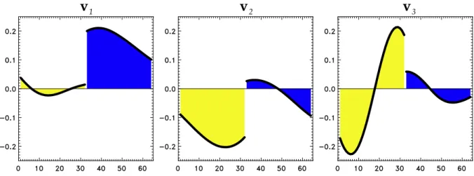
1
v
v
2v
3Fig. 8. The first three principal components of vBS−ALcovariance matrix computed with MI =MO =32. The input (vBS) portion of
vector is shown in yellow, while the output (AL) part is indicated by the blue color.
3 Embedding analyses of magnetospheric dynamics Previous studies pointed out that the magnetospheric dynam-ics has different properties at different scales. The dimen-sion analysis of AE data (Vassiliadis et al., 1990) showed that the correlation dimension saturates at low values, which indicates the global nature of substorm dynamics. It was also shown that a large portion of the AE time series can be de-scribed by low dimensional dynamical models (Vassiliadis et al., 1995). However, it was also demonstrated that if all in-teraction scales are taken into account, then the AE time se-ries does not have a low correlation dimension (Prichard and Price, 1992). Using the coast-line dimension analysis Sit-nov et al. (2000) showed that the low dimensional behavior can be derived only for the fixed range of the largest pertur-bation scales, while the singular value spectrum of data has a power-law shape typical for the colored noise. The sub-sequent analyses of the multi-scale constituent of AL also indicated that it has dynamical and statistical properties sim-ilar to the time series of high dimensional noise (Ukhorskiy et al., 2002a).
The main goal of our work is to develop a comprehensive model that can account for both global and high dimensional constituents of the solar wind-magnetosphere coupling dur-ing substorms. The basis of this model is provided by the em-bedding analysis discussed in previous sections. Our method yields the mean-field dimensions of the system that are used for constructing low dimensional dynamical model to run it-erative predictions of the observed time series (Ukhorskiy et al., 2002a). Moreover, it also yields the distribution func-tion of the high dimensional dynamical constituent in the re-constructed phase space. In this section we show how this distribution function can be used for studying the structure of a low dimensional dynamical attractor and discuss its ap-plication to probabilistic predictions of the magnetospheric dynamics.
Previous studies of the solar wind-magnetosphere cou-pling discussed different choices of the solar wind input
pa-rameters for the magnetospheric dynamics. For the model-ing of AL and AU indices Clauer et al. (1981) considered the solar wind convective electric field vBS, v2BS and the
solar wind coupling parameter ε = vB2l02sin4(θ /2) (Aka-sofu, 1979). They found that the moving average linear fil-ters based on these three inputs have the similar prediction accuracy of 40%. Vassiliadis et al. (1995) reported that the local-linear filters driven by vBS, vB2l02sin4(θ /2) and vBz
yield a comparable predictability of AL. For the predictions of high geomagnetic activity the best results were achieved with unrectified vBz input. In this study the solar wind
in-put is quantified by vBS, while the magnetospheric response
is represented by the AL index. This allows for the direct comparison of our embedding analysis with earlier results of Sitnov et al. (2000, 2001), obtained for vBS −ALtime
series. All analyses were carried out using the correlated database of solar wind and geomagnetic time series compiled by Bargatze et al. (1985). The data are solar wind param-eters acquired by IMP 8 spacecraft and simultaneous mea-surements of auroral indices with a resolution of 2.5 minutes. The database consists of 34 isolated intervals, which contain 42 216 points in total. Each interval represents the isolated interval of auroral activity preceded and followed by at least two-hour-long quiet periods (vBS ≈0, AL < 50 nT). Data
intervals are arranged in the order of increasing geomagnetic activity. In order to use both vBSand AL data in joint
input-output phase space, their time series are normalized to their standard deviations.
To determine the mean-field dimensions of the magneto-spheric dynamics we follow the prescription of our method and estimate the embedding dimensions of the vBS −AL
time series after carrying out the ensemble averaging in the embedding space. The distribution functions of Dnare
cal-culated for different values of N N , which set the range of scales participating in the averaging (Fig. 7). The distribu-tion funcdistribu-tion calculated for averaging over N N = 3 has a power-law shape. This indicates that at the finest scales the
1924 A. Y. Ukhorskiy et al.: Global and multi-scale features of magnetospheric dynamics 3
x
2x
x
2 3x
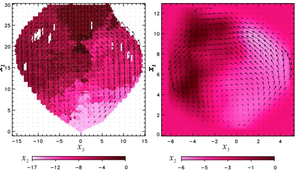
Fig. 9. The coherent dynamics in three-dimensional subspace spanned by the leading principal components of vBS−ALcovariance matrix.
(a) The dynamical manifold is derived with the use of the two-dimensional distribution function ρ(x1, x3)calculated for the whole Bargatze
et al. (1985) database with N N = 300. The points of the surface are associated with the maxima of the conditional probability function
ρ(x2|x1, x3) ∼=ρ(x2(k)). (b) Smoothed dynamical manifold calculated for the first 20 intervals of Bargatze et al. (1985) database by Sitnov
et al. (2001).
dynamics in the system is irregular and cannot be embedded in a finite-dimensional space. Only after a substantial range of scales is smoothed away (N N > 100) does the averaged system start to exhibit a low dimensional behavior. Thus, for N N = 100 the mean-field dimension is D = 7, and for
N N =250, D = 3. To define which embedding parameters are optimal for modeling the evolution of the system we con-struct the dynamical model (8) and then calculate N MSE for different values of (D, N N ). For (3, 250) N MSE = 0.63 and for (7, 100) the error value is smaller, N MSE = 0.57.
After the optimal embedding parameters (D, N N ) are chosen, the probability density function of the attractor states can be estimated as Eq. (12). Since it is a distribution func-tion in D-dimensional reconstructed phase space, it can be used for studying the collective behavior of the system. The global dynamics of the system is described by the moments of the distribution function. Thus, the zeroth order term in dynamical model (8), viz. the center of mass, is nothing but its first moment. The distribution function can also be used for visualizing the low dimensional component of the solar wind-magnetosphere coupling. Earlier procedures of visualizing the global part of the magnetospheric dynamics (Sitnov et al., 2000; Sitnov et al., 2001) involved a num-ber of cumnum-bersome procedures, such as the removal of the hysteresis loops and the smoothing of the resultant 2-D sur-face. Our new systematic approach resolves these problems by substituting the raw data by its probability density func-tion in the reconstructed space, whose dimension is consis-tent with the level of averaging and the level of noise. To compare our results with the phase portrait obtained by
Sit-nov et al. (2001), we plot the data in three-dimensional space given by the principal components v1, v2and v3of vBS−AL
covariance matrix. For a better comparison the principal components were calculated for the matrices computed with the same MI = MO = 32 number of delays as was used
by Sitnov et al. (2001). Vectors v1, v2 and v3 are shown
in Fig. 8. The delay vector projections x1 , x2and x3 onto
v1, v2and v3roughly correspond to one-hour average values
of input (normalized vBS), output (normalized AL) and the
first time derivative of the input (for details, see Sitnov et al., 2000). To visualize the data we use x1−x3projection as the
support plane, where the distribution function ρ(x1, x3)is
introduced according to Eq. (12), with N N = 300 obtained by the mean-field dimension analysis. Then, at any given point (x1, x3)the conditional probability function of x2can
be estimated as the probability density function of x2(k) cor-responding to the nearest neighbors of that point:
ρ(x2|x1, x3) ∼=ρ(x2(k)), xk =(x1(k), x3(k)) ∈ N N . (16)
The points of conditional probability maxima calculated at the mesh points of the regular grid set represent the surface corresponding to the most probable states of the system in three dimensional phase space. Such a surface calculated for the whole Bargatze database is presented in Fig. 9a. To visu-alize the evolution of the system along this surface we plot a two-dimensional velocity field, viz. the average flow velocity in a x1−x2plane calculated using the distribution function
ρ(x1, x2). As can be seen from the plot the structure of the
surface and the corresponding circulation flows are very sim-ilar to those obtained by Sitnov et al. (2000). This simsim-ilarity
is even more notable, since the phase portrait on the right was derived only for the first 20 intervals of the database, corre-sponding to the low and medium levels of substorm activity. At the same time, the robustness of our technique yields the phase portrait for the whole data containing both low and high activity intervals. The most probable substorm cycles are confined to the two-level surface, with the fracture going roughly along the x3=0 axis. Two levels of the surface can
be associated with the ground and exited states of the sys-tem. The typical substorm cycle starts with an increase in the average input x1, while the average output x2is constant
or slowly decreasing, viz. the system is in its ground state. At the same time the average input rate x3first increases and
then decreases to small values. Then the output component falls rapidly to negative values at almost constant input pa-rameters, which corresponds to the transition to the exited state. The recovery of the system to its ground state involves the decrease in x1while the magnitude of x3first increases
and then falls to zero values.
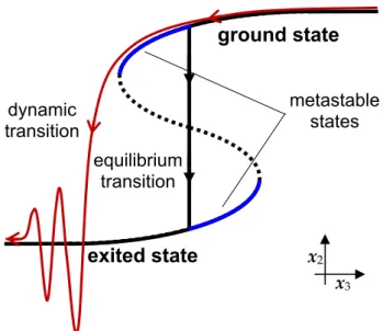
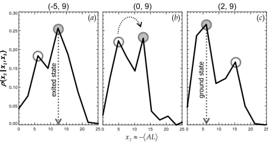
It was pointed out before (Sitnov et al., 2000) that both the surface and the corresponding circulation flows are close to the scheme of the inverse bifurcation (Lewis, 1991). This implies that the smooth manifold underlying the global por-tion of system’s dynamics has a folded structure known in mathematics as a cusp catastrophe manifold (Gilmore, 1993) and in the physics of non-equilibrium phase transitions as a coexistence surface separating deferent states of matter (Gunton et al., 1983). In the case of the quasi-static phase transitions in equilibrium systems the corresponding coex-istence surface does not have such a folded structure. In these systems the order parameter is a single-valued func-tion of control parameters (Fig. 10). The fold appears only in the non-equilibrium case, when the system is driven far from the steady-state equilibrium by the rapid changes in the control parameters. As a result the metastable states, like “overcooled” steam and “overheated” fluid, become possible and depending on its dynamical history, the system may be in two or more different states under the same set of control pa-rameters. This dynamical phenomenon known as hysteresis explains the observed irregular structure of the transition line (see Fig. 9a). It also strongly complicates the reconstruction and visualization of the global dynamical constituent (Sit-nov et al., 2000). In the present approach this problem is overcome with the use of the distribution function. To visu-alize the large-scale behavior we follow the dynamics of the distribution function maxima which is somewhat analogous to the Maxwell convention in bifurcation theory (Gilmore, 1993) and thus establishes the parallel with the equilibrium coexistence surface. The existence of the multiple maxima is attributed to the dynamical hysteresis. The points on the sur-face corresponding to the transitions between the ground and exited states are identified by the change in the position of the global maxima. Figure 11 shows the distribution function of
x2calculated at three points along the cut of the surface by
the x1 =9 plane. In all three cases it has a typical
double-peak structure which indicates the existence of hysteresis. Figure 10 illustrates the system’s transition from the ground
ground state
exited state
equilibrium
transition
dynamic
transition
metastable
states
x
2x
3Fig. 10. The diagram of different transitions in a two-level system.
The coexistence manifold and corresponding transitions from the ground to the exited state are shown in x1−x3plane. Equilibrium
transitions correspond to the straight line connecting two branches associated with different states. The metastable states correspond to the blue segments of the manifold. An example of a typical dynamic transition which deviates from the equilibrium manifold is shown in red.
to the exited state, as identified by changes in the shape of the distribution function. According to criterion (15) the distri-bution function in Fig. 10c corresponds to the ground state of the system. The distribution function in Fig. 10b corresponds to the moment when the transition to the exited state was just made. And finally, the function in Fig. 10a corresponds to the fully developed exited state of the system. Thus, the distribution function and its moments can be effectively used to predict, visualize and analyze the global portion of the so-lar wind-magnetosphere coupling. Moreover, the description provided by the distribution function is not restricted to the low dimensional dynamical constituent. Indeed, if the distri-bution function and its evolution with the input parameters are derived from the observed time series, then, in principal, it gives the full description of the collective behavior in the system. The dynamics of its first moment corresponds to the mean-field dynamical model, which yields iterative predic-tions of the observed time series. As was discussed before (Ukhorskiy et al., 2002a), the dynamical model leaves out a significant portion of the dynamics. Indeed, in order to extract the coherent component from the time series gener-ated by a system with some randomness, the model is forced to carry out the phase space averaging over a wide range of scales. Therefore, the output of the model comes inher-ently smoothed and cannot grasp the large peaks and sharpest changes in data. As will be discussed in forthcoming publi-cations this problem can be partially resolved with the use of a distribution function, which yields the probabilistic de-scription of the multi-scale dynamical constituent. It can be
1926 A. Y. Ukhorskiy et al.: Global and multi-scale features of magnetospheric dynamics AL x2≈− (0, 9) (-5, 9) (2, 9) ground state exited state (a) (b) (c)
Fig. 11. Evolution of the distribution function at the different stages of substorm. Double-peak shape of the function indicate the existence
of dynamical hysteresis. (c) The dominance of the left maximum indicates that the system is in the ground state (growth phase). (b) The equality of the maxima corresponds to the transition from the ground to the exited state (expansion phase). (a) Predominance of the right maximum indicates that the system is in the exited stated (late expansion or early recovery phases).
used to estimate the deviation of the data from the output of the deterministic model and thus can be used for probabilis-tic predictions. Incorporating this distribution function in the space weather prediction tools has important implications for space weather forecasting.
4 Conclusions
The solar wind-magnetosphere coupling during substorms exhibits dynamical features in a wide range of spatial and temporal scales. The large-scale portion of the magneto-spheric dynamics is coherent and well organized, while many small-scale phenomena appear to be multi-scale. Most of the contemporary approaches to the data-derived modeling of magnetospheric substorms do not account for the coexis-tence of global and multi-scale phenomena and thus do not provide a complete description of the observed time series. Low dimensional dynamical models effectively extract the time series constituent generated by the large-scale coher-ent behavior, but are unable to predict the features associ-ated with high dimensional multi-scale dynamics. At the same time, SOC-like models can reproduce a variety of the scale-free power spectra typical for the multi-scale portion of the observed time series, but are incapable of relating them to the specific global features of the actual magnetospheric dynamics and variations in the solar wind input. The goal of our work is to combine the global and multi-scale fea-tures of the solar wind-magnetosphere coupling in a single data-derived model. For this purpose we combined the deter-ministic methods of nonlinear dynamics with the distribution function technique of statistical physics. In this paper we analyzed to what extent the magnetospheric dynamics can be predicted with the use of the low dimensional
dynami-cal models and at what point the statistidynami-cal description is re-quired. This question was addressed by embedding analyses of vBS−ALtime series. A large portion of magnetospheric
dynamics is driven by the solar wind input whose time se-ries have scale-free power spectra. Thus, for its embedding analyses we introduce a new method of determining the em-bedding parameters of the input-output time series generated by random dynamical systems. To test our method we used several well-known autonomous as well as input-output dy-namical systems, with and without noise contamination.
According to our embedding analysis, the multi-scale properties of the vBS −AL time series are very different
from the multi-scale properties of low dimensional chaotic systems, like the Lorenz attractor or Mackey-Glass system, in which the scale-invariance is reconciled with low dimen-sionality due to the fractal nature of their attractors. Due to the scale-invariance of its driver and/or due to its own complexity, the magnetospheric dynamics generate time se-ries which contain a small-scale component with properties of high dimensional colored noise. This high dimensional constituent destroys the coherence of the system’s dynam-ics in the phase space, smearing trajectories in some vicinity of the manifold containing the dynamical attractor. Thus, if the time series are considered at the smallest possible scale, they do not allow embedding in any finite dimension. To extract the large-scale regular component from the time se-ries, the ensemble averaging over a number (N N ) of near-est neighbors, which defines the range of scales affected by noise in D-dimensional embedding space, is carried out. This smoothes away the small- scale high dimensional com-ponent and unfolds the trajectories of the averaged system in D-dimensional embedding space. The higher the value of N N , the wider the range of scales which are smoothed away and the smaller the effective dimension D of the