The tropical forest and fire emissions experiment: laboratory fire measurements and synthesis of campaign data

(1)

HAL Id: hal-00303375

https://hal.archives-ouvertes.fr/hal-00303375

Submitted on 3 Mar 2008

HAL is a multi-disciplinary open access

archive for the deposit and dissemination of sci-entific research documents, whether they are pub-lished or not. The documents may come from teaching and research institutions in France or abroad, or from public or private research centers.

L’archive ouverte pluridisciplinaire HAL, est destinée au dépôt et à la diffusion de documents scientifiques de niveau recherche, publiés ou non, émanant des établissements d’enseignement et de recherche français ou étrangers, des laboratoires publics ou privés.

The tropical forest and fire emissions experiment:

laboratory fire measurements and synthesis of campaign

data

R. J. Yokelson, T. J. Christian, T. G. Karl, A. Guenther

To cite this version:

R. J. Yokelson, T. J. Christian, T. G. Karl, A. Guenther. The tropical forest and fire emissions experiment: laboratory fire measurements and synthesis of campaign data. Atmospheric Chemistry and Physics Discussions, European Geosciences Union, 2008, 8 (2), pp.4221-4266. �hal-00303375�

(2)

ACPD

8, 4221–4266, 2008

Tropical forest fire emissions R. J. Yokelson et al. Title Page Abstract Introduction Conclusions References Tables Figures ◭ ◮ ◭ ◮ Back Close

Full Screen / Esc

Printer-friendly Version

Interactive Discussion Atmos. Chem. Phys. Discuss., 8, 4221–4266, 2008

www.atmos-chem-phys-discuss.net/8/4221/2008/ © Author(s) 2008. This work is distributed under the Creative Commons Attribution 3.0 License.

Atmospheric Chemistry and Physics Discussions

The tropical forest and fire emissions

experiment: laboratory fire measurements

and synthesis of campaign data

R. J. Yokelson1, T. J. Christian1, T. G. Karl2, and A. Guenther2

1

University of Montana, Department of Chemistry, Missoula, MT, 59812, USA

2

National Center for Atmospheric Research, Boulder, CO, USA

Received: 3 January 2008 – Accepted: 31 January 2008 – Published: 3 March 2008 Correspondence to: R. J. Yokelson (bob.yokelson@umontana.edu)

(3)

ACPD

8, 4221–4266, 2008

Full Screen / Esc

Interactive Discussion Abstract

As part of the Tropical Forest and Fire Emissions Experiment (TROFFEE), tropical for-est fuels were burned in a large, biomass-fire simulation facility and the smoke was characterized with open-path Fourier transform infrared spectroscopy (FTIR), proton-transfer reaction mass spectrometry (PTR-MS), gas chromatography (GC),

GC/PTR-5

MS, and filter sampling of the particles. In most cases, about one-third of the fuel chlo-rine ended up in the particles and about one-half remained in the ash. About 50% of the mass of non-methane organic compounds (NMOC) emitted by these fires could be identified with the available instrumentation. The lab fire emission factors (EF, g com-pound emitted per kg fuel burned) were coupled with EF obtained during the TROFFEE

10

airborne and ground-based field campaigns. This revealed several types of EF depen-dence on parameters such as the ratio of flaming to smoldering combustion and fuel characteristics. The synthesis of data from the different TROFFEE platforms was also used to derive EF for all the measured species for both primary deforestation fires and pasture maintenance fires – the two main types of biomass burning in the Amazon.

15

Many of the EF are larger than those in widely-used earlier work. This is mostly due to the inclusion of newly-available, large EF for the initially-unlofted smoldering emis-sions and the assumption that these emisemis-sions make a significant contribution (∼40%) to the total emissions from pasture fires. The TROFFEE EF for particles with aero-dynamic diameter <2.5 microns (EFPM_2.5) is 14.8 g/kg for primary deforestation fires

20

and 18.7 g/kg for pasture maintenance fires. These EFPM2.5 are significantly larger

than a previous recommendation (9.1 g/kg) and lead to an estimated pyrogenic pri-mary PM_2.5source for the Amazon that is 84% larger. Regional through global budgets for biogenic and pyrogenic emissions were roughly estimated. Coupled with previous measurements of secondary aerosol growth in the Amazon and source apportionment

25

studies, the regional budgets suggest that ∼5% of the total mass of the regionally gen-erated NMOC end up as secondary organic aerosol within the Amazonian boundary layer within 1–3 days. The global budgets confirm that biogenic emissions and biomass

(4)

ACPD

8, 4221–4266, 2008

Full Screen / Esc

Interactive Discussion burning are the two largest global sources of NMOC with an estimated production of

approximately 1000 and 500 Tg/yr, respectively. It follows that plants and fires may also be the two main global sources of secondary organic aerosol. A limited set of emission ratios (ER) is given for sugar cane burning, which may help estimate the air quality impacts of burning this major crop, which is often grown in densely populated areas.

5

1 Introduction

Biomass burning and biogenic emissions are the two largest sources of volatile or-ganic compounds (VOC) and fine particulate carbon in the global troposphere. Tropical forests produce about one-third of the global biogenic emissions and tropical deforesta-tion fires account for >15% of the global biomass burning (Andreae and Merlet, 2001;

10

Kreidenweis et al., 1999; Guenther et al., 2006). The Tropical Forest and Fire Emis-sions Experiment (TROFFEE) used laboratory measurements (in October of 2003) followed by airborne and ground based field campaigns during the 2004 Amazonian dry season to quantify the emissions from tropical deforestation fires, other tropical fires, and tropical vegetation (Yokelson et al., 2007a).

15

The laboratory experiment involved measuring the emissions from 32 fires that burned tropical forest fuels and a few other fuels (e.g. sugar cane, pine needles, and savanna grass). The lab work was conducted for a number of reasons. (1) Deter-mine the proton-transfer reaction mass spectrometry (PTR-MS) sampling protocol for the field campaign (by identifying the significant mass/charge (m/z) ratios observed

20

by PTR-MS in smoke). (2) Intercomparing PTR-MS with open-path Fourier transform infrared spectroscopy (FTIR) and gas chromatography coupled to PTR-MS (GC/PTR-MS). The intercomparison showed good agreement in most cases, but also revealed important biomass burning emissions that are difficult to measure by FTIR (due to in-terference by water lines) or PTR-MS (due to low proton affinity or sampling losses).

25

(3) The GC/PTR-MS and FTIR measured the fractional contribution for fire-emitted species that appear at the same m/z in the PTR-MS (Karl et al., 2007a).

(5)

ACPD

8, 4221–4266, 2008

Full Screen / Esc

Interactive Discussion Laboratory studies offer some other advantages as well. Typically, smoke

concentra-tions are higher and more instrumentation can be deployed in the lab than in the field. (For TROFFEE additional lab techniques included open-path FTIR, GC-PTR-MS, and particle collection on filters.) Both of the above advantages mean that more species can be quantified. In the lab one can capture and probe all the smoke from a whole fire,

5

while in the field the vast majority of the smoke must go unsampled. Also, in the field the possibility exists for over-estimating flaming emissions from airborne platforms or under-estimating them from ground-based platforms. Laboratory studies also provide the opportunity to perform mass-balance studies that account for the fate of various el-ements in the fuel. Finally, in TROFFEE, the lab studies provided the chance to study

10

the emissions from some important fuel types that we were unable to sample in the field (e.g. sugar cane). The most serious disadvantage of a laboratory fire simulation is the possibility that the lab fire emissions are different from fire emissions produced in the field. This is especially critical for tropical forest fuels as it is impractical to burn a diverse suite of large diameter tropical logs in the lab.

15

In this paper we present and discuss: (1) a partial accounting of the fate of the chlo-rine and potassium in the biomass fuel in our lab fires, (2) an overview and synthesis of the lab, ground, and airborne results to derive recommended EF for primary tropical deforestation fires and tropical pasture maintenance fires, (3) approximate budgets for vegetative and fire emissions of NMOC at the Amazon-basin scale and global scale,

20

and (4) excess emission ratios (ER) and emission factors (EF) for sugar cane.

2 Experimental

2.1 Combustion facility

The combustion facility at the Fire Sciences Laboratory measures 12.5 m×12.5 m×22 m high. A 1.6 m diameter exhaust stack with a 3.6 m inverted

25

(6)

ACPD

8, 4221–4266, 2008

Full Screen / Esc

Interactive Discussion is continuously pressurized with outside air that has been conditioned for temperature

and humidity, and is then vented through the stack, completely entraining the emis-sions from fires burning beneath the funnel. The fires were burned on a continuously weighed fuel bed. A sampling platform surrounds the stack at 17 m elevation where all the temperature, pressure, trace gas, and particle measurement equipment for this

5

experiment was deployed except background CO2 (LICOR 6262). The emissions are

well mixed in the stack at the height of the sampling platform. Additional details can be found in Christian et al. (2004).

2.2 Fuel types and characterization

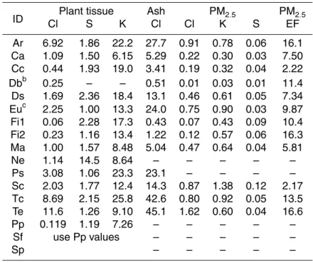
Table 1 presents a list of fuel types, with genus and species where applicable, as well

10

as a two-letter abbreviation for each fuel type (for reference purposes within this study). The list includes 16 tropical species provided by the University of Colorado, one dambo grass species obtained for previous laboratory experiments with savanna fuels (Chris-tian et al., 2003) and three local, temperate forest tree species used primarily in the intercomparison portion of this work (Karl et al., 2007a). The plant material was limited

15

to leaves, twigs, and branches of less than ∼30 mm diameter. This was intended to represent the small diameter fuels of typical, global deforestation fires; but does not include the large diameter logs, which contributed to the emissions measured in the field campaign. Table 1 also shows the dry weight percentage of carbon, hydrogen, and nitrogen in the bulk plant tissue and ash; the percentage of carbon in the organic

20

(burnable) plant material (ash-free %C); and the fuel moisture at the time of the fire (100×(wet-dry)/dry)). We determined the production of ash and partially burned ma-terial by manually weighing these residuals. We determined the fuel moisture content by measuring the mass loss from pre-fire sub-samples after drying them overnight at 90◦C.

25

The results of additional elemental analysis by an independent laboratory (Columbia Analytical Services, Inc.) are given in Table 2. Chlorine and sulfur were determined via Parr bomb combustion and ion chromatography of the leachate for both the plant tissue

(7)

ACPD

8, 4221–4266, 2008

Full Screen / Esc

Interactive Discussion and the ash from the fires. Plant tissue potassium was determined via acid digestion

and ICP-OES (Inductively Coupled Plasma – Optical Emission Spectroscopy).

2.3 Open-path FTIR

The open path Fourier transform infrared spectrometer (OP-FTIR) was positioned on the sampling platform so that the open white cell spanned the stack directly in the

5

rising emissions stream for continuous (0.83 s resolution) scanning. The OP-FTIR sys-tem (Yokelson et al., 1997) includes a MIDAC model 2500 spectrometer; an open path White cell with 1.6 m base path, and an MCT (mercury-cadmium-telluride), LN2

-cooled detector. The path length was set to 57.7 m and the spectral resolution was 0.5 cm−1. Before each fire, we scanned for 2–3 min to obtain a background spectrum,

10

and then made absorbance spectra at 0.83 s resolution using this background spec-trum. We then averaged every ∼10 absorbance spectra under conditions of slowly changing temperature and emissions to increase the signal to noise ratio.

We used classical least squares spectral analysis (Griffith, 1996; Yokelson and Bertschi, 2002) to retrieve excess mixing ratios for water (H₂O), methane (CH₄),

15

methanol (CH3OH), ethylene (C2H4), phenol (C6H5OH), acetone (CH3C(O)CH3),

iso-prene (C5H8), hydrogen cyanide (HCN), furan (C4H4O), nitric oxide (NO), nitrogen

dioxide (NO₂), and formaldehyde (HCHO). We used spectral subtraction (Yokelson et al., 1997) to retrieve excess mixing ratios for water (H2O), ammonia (NH3), formic

acid (HCOOH), acetic acid (CH3COOH), glycolaldehyde (CH2(OH)CHO), acetylene

20

(C₂H₂), and propylene (C₃H₆). While CO₂ and CO are accurately measured by OP-FTIR (Goode et al., 1999), due to the large volume of data, we opted to use the conve-nient, synchronized data for these molecules from the real-time instruments (Sect. 2.5). The molecules discussed above account for all the significant features observed from 600–3400 cm−1in all the IR spectra. The detection limit for most gases was 10–50 ppb

25

at the most common time resolution used (∼8 s). The typical uncertainty in an FTIR mixing ratio is ±5% (1 σ) due to calibration or the detection limit (2 σ), whichever is greater.

(8)

ACPD

8, 4221–4266, 2008

Full Screen / Esc

Interactive Discussion 2.4 PTR-MS

Background information on PTR-MS has been given in detail by Lindinger et al. (1998). The PTR-MS setup used here is described in more detail by Karl et al. (2007a). Briefly, H3O+ is used to ionize volatile organic compounds (VOC) whose proton affinity is

greater than that of water. A flow-drift-tube system guarantees that the reactions take

5

place under well defined conditions so that product ion count rates are correlated to VOC absolute concentrations according to Eq. (1):

H3O++ VOC

k

−→VOCH++ H₂O (1)

The proton transfer rate constants k are large, corresponding to the collision-limited values (≫10−9cm3s−1) (Praxmarer et al., 1994). The ratio of the electric field strength

10

to the buffer gas density in the drift tube is kept at about 120 Townsend to avoid strong clustering of H₃O+ ions with water. In this study the mass analyzer of the PTR-MS was a conventional quadrupole mass filter (QMG 422, Balzers, Lichtenstein) with a mass range up to ∼500 amu (atomic mass units). Because ion transmission of the quadrupole decreases with mass, scans were conducted only up to 205 amu. More

15

details on instrument performance and calibration procedures can be found in Karl et al. (2007a).

In order to enhance the specificity of the VOC partitioning observed by the PTR-MS, we also used a gas chromatograph in line before the PTR-MS (GC/PTR-MS). If more than one compound was observed at a single m/z, the peaks were identified based on

20

a combination of GC retention times and PTR-MS VOC fragmentation data. Sample air for this technique was taken either directly from the stack or from stainless steel canisters collected during a fire and analyzed immediately afterward. The sample was trapped on Tenax for 10 min at −10◦C, then desorbed by heating to 200◦C onto a 50 m HP-624 column (Shimadzu GC instrument), and analyzed using the PTR-MS

instru-25

ment as the detector (Greenberg, 1994). Retention times were obtained individually by injecting pure standards. The contribution of various compounds to specific m/z channels is treated in more detail by Karl et al. (2007a).

(9)

ACPD

8, 4221–4266, 2008

Full Screen / Esc

Interactive Discussion In these experiments the PTR-MS frequently scanned all m/z up to 205. The

individ-ual species that could be quantified typically accounted for ∼72% of the total ion signal up to 205 m/z that was observed by this instrument. Thus about 70% of the NMOC that were emitted by these fires and detected by the PTR-MS have been individually quantified (on a molar basis). This is an important consideration in photochemical

5

modeling of smoke chemistry as shown by Trentmann et al. (2005) who successfully modeled the O₃formation observed in a smoke plume after the measured initial NMOC were increased by 30% as a proxy for the unmeasured NMOC. In addition, most of the unidentified species occur at heavier masses, which are also transmitted less efficiently through the PTR-MS quadrupole. Therefore, on a mass basis, only about 50% of the

10

NMOC emitted by these fires were individually quantified. This is important in estimat-ing local-global pyrogenic budgets (e.g. Sect. 3.3).

2.5 Particle, CO2, and CO measurements

Stack air was drawn at 30 L min−1through dielectric tubing and a cyclone that passed only particles with an aerodynamic diameter less than 2.5 µm (PM_2.5) onto Teflon

fil-15

ters. The filters were analyzed gravimetrically by the US Forest Service (Trent et al., 2000) and then by X-Ray Fluorescence (XRF) at an independent laboratory for chlo-rine, potassium, and sulfur. The same sample flow was used for continuous, in-stack CO2(LICOR 6262) and CO (TECO 48C) measurements. The TECO and two LICORs

(including a floor-level, background air monitor) were calibrated with NIST traceable

20

standards. We continuously monitored fuel mass and stack temperature, pressure, and flow with 2 s resolution.

2.6 Calculation of modified combustion efficiency and emission factors

The excess mixing ratio of any species above background that was due to the fire at any moment was assumed to be the mixing ratio of the species measured in the

25

(10)

ACPD

8, 4221–4266, 2008

Full Screen / Esc

Interactive Discussion adjacent to the fuel bed or in the stack before and after the fire. These excess mixing

ratios are designated with a capital Greek letter delta (e.g. ∆CO). Dividing the fire-integrated CO emissions (∆CO) by the fire-fire-integrated CO2 emissions (∆CO2) yields

the fire-integrated ∆CO/∆CO2molar emission ratio (ER). The ∆CO/∆CO2ER and the

molar modified combustion efficiency (MCE, ∆CO2/(∆CO2 + ∆CO) are used to

indi-5

cate the relative amount of flaming and smoldering combustion during a fire. Higher ∆CO/∆CO2or lower MCE indicates more smoldering (Ward and Radke).

For any carbonaceous fuel, a set of molar ER to CO₂that includes the major carbon-containing species (i.e. CO, CH4, a suite of NMOC, and particle carbon) can be used

to calculate emission factors (EF, g of compound emitted per dry kilogram of fuel

con-10

sumed) by the carbon mass balance method (Yokelson et al., 1996). This method assumes that all the burned carbon is volatilized and detected, an assumption that probably inflates the EF by 1–2% (Andreae and Merlet, 2001). In our calculations we used the measured ash-free fuel carbon percentage (Table 1) and assumed that the particles were 60% C by mass (Ferek et al., 1998).

15

3 Results

3.1 Chlorine and potassium in fuels, particles, and ash

For 10 of the 13 tropical fuel types for which we obtained both PM2.5and chlorine data,

approximately one third of the fuel chlorine was accounted for by the chlorine in the PM2.5 (Fig. 1a, upper (black) trend line). This is in good agreement with previous

re-20

sults for African fuels (Christian et al., 2003). Keene et al. (2006) also found that one third of the fuel chlorine ended up in the particles in their laboratory burns of tropical fuels (their Fig. 6b). However, 3 of 13 fuels in our current study did not adhere to this trend (Artocapus altilus, tropical composite, and Terminalia catappa). Fires with these 3 fuels had higher than average particle emissions and higher than average Cl

con-25

(11)

ACPD

8, 4221–4266, 2008

Full Screen / Esc

Interactive Discussion The net result when these anomalous fires were included in the regression was that

the particles only accounted for about 16% of the fuel chlorine (Fig. 1a, lower (red) trend line). A cause for the “low-yield” points could not be determined. We have no information on the potentially varying chemical forms of the fuel or particle chlorine. If the Cl in the PM_2.5 was more volatile for these fires, it may have evaporated before

5

analysis/detection. We do not know if these three fires perhaps emitted an unusual amount of large particles that might have contained chlorine, but were intercepted by the cyclone. Re-examination of the IR spectra from these three fires did not reveal ab-sorption features for hydrochloric acid (HCl) or chlorinated hydrocarbons, which might have indicated a gas-phase fate for some of the fuel Cl. We conclude that about 33%

10

of the fuel chlorine often ends up in the particles but that important exceptions may occur.

In any case, the chlorine in the particles does not account for 67% or more of the fuel chlorine. Based on their similar results, Christian et al. (2003) hypothesized that most of the fuel chlorine remains in the ash or is emitted in unidentified trace gases. Thus,

15

in this study we measured the yield and chlorine content of the ash and found that about one-half (48%) of the fuel chlorine remained in the ash (Fig. 1b). With this new information, 64–83% of the fuel chlorine can be accounted for with the “typical” case being over 80%. The remaining chlorine may be unidentified gases or volatile forms of particle chlorine. For instance, HCl could be initially present in the particles (thus

20

escaping detection as a trace gas by FTIR in the stack), but then evaporate during filter storage before elemental analysis.

Treatment of the potassium data for PM_2.5in a similar fashion as Fig. 1 shows particle K to be relatively independent of fuel K (r2∼_{=0.4). This is expected based on the} find-ings of Ward and Hardy (1991) who showed that the emissions of fine particle K were

25

strongly associated with the proportion of flaming combustion during a fire (see their Fig. 6). Our average EF for fine particle potassium was 0.62±0.35 (g K in PM2.5/kg dry

fuel) obtained at an average MCE of 0.949. This is about twice the EFK (0.29±0.22) reported by Andrea and Merlet (2001) for tropical forest fires, but at an average MCE

(12)

ACPD

8, 4221–4266, 2008

Full Screen / Esc

Interactive Discussion of 0.906 that indicates less flaming combustion. Thus these two results are consistent

with what we know about the emissions behavior for K and it should be clear that the mix of flaming and smoldering combustion needs to be considered when regional PM source apportionment based on K is performed (Ward and Hardy, 1991). Finally, we note that the average mass of K in PM_2.5 as a percentage of the total mass of K in the

5

burned fuel in this study was 4.6%±3.1%. Kauffman et al. (1998) found that 82±12% of fuel K remained in the ash.

3.2 Synthesis of TROFFEE laboratory, airborne, and ground-based measurements of emission factors

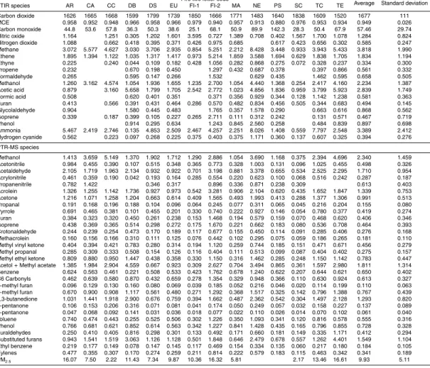
Table 3 presents our fire-average MCE and emission factors for each tropical fuel type

10

burned in the laboratory. The trace gas data are segregated to indicate the source of the measurement – FTIR or PTR-MS. Consideration of this data, along with the air-borne and ground-based EF measurements obtained in the field campaigns in Brazil (Yokelson et al., 2007a; Christian et al., 2007), provides an unprecedented amount of information on the relationship between the combustion characteristics and the

emis-15

sions produced as well as the chemistry of these emissions. Each study offers ad-vantages in understanding the overall picture. The airborne and ground-based mea-surements are of “real” fires during the peak of the 2004 biomass burning season in Brazil, but represent sampling only a part of the emissions from each fire. Explicitly, the ground-based measurements are of initially-unlofted emissions produced by residual

20

smoldering combustion of logs, which is reflected in their average MCE of 0.788±0.059. A large part of these emissions is later lofted by thermal or frontal processes, but on average they may have a shorter atmospheric lifetime than the initially lofted emissions, which are also amenable to airborne sampling. The airborne measurements sample a mix of flaming and “entrained” smoldering emissions, but necessarily omit the

ini-25

tially unlofted emissions sampled from the ground. They have a higher average MCE of 0.910±0.021. The laboratory experiments captured smoke over the course of the whole fire. The laboratory setting also allowed more comprehensive measurements

(13)

ACPD

8, 4221–4266, 2008

Full Screen / Esc

Interactive Discussion (e.g. open-path FTIR, GC-PTR-MS, particle collection on filters, and monitoring of all

the PTR-MS mass channels during the fires (as opposed to a reduced selection neces-sitated by the briefer times in smoke in the airborne campaign)). However, the lab fires are not authentic tropical fires. In particular, the lab fire average MCE of 0.949±0.026 likely reflects the absence of smoldering large-diameter logs in the fuel mix. From a

5

fuels perspective, the lab-fires primarily focused on the foliage and twigs, the ground-based measurements on large-diameter logs, and the airborne measurements on a mix of the small and large fuels.

Many earlier studies have shown plots of emission factors vs. MCE for measure-ments conducted on fires that were burning mostly smaller diameter fuels. For

ex-10

ample, see the plots for airborne measurements of savanna fire EF in Yokelson et al. (2003), or lab measurements of savanna fire EF in Christian et al. (2003). In that work a high degree of correlation between EF and MCE was observed (positive cor-relation for compounds produced by flaming combustion and negative corcor-relation for smoldering compounds). Also a more restricted range of MCE was observed (0.910–

15

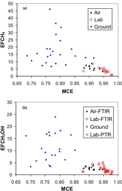
0.975), which probably represented the real range of fire-integrated MCE occurring in savanna fires. In discussing TROFFEE samples of deforestation fires, we will use the same “EF versus MCE” framework to probe a much wider range of conditions. In Figs. 2–4, for selected compounds, we show all the EF versus MCE from all three TROFFEE platforms on the same plot. This shows, in one view, how the emission

20

factors are affected by a broad range of MCE and the fuel differences. All but three of the ground-based measurements (indicated by blue circles) are at an MCE below ∼0.85 (mostly smoldering) and the fuel is almost exclusively large diameter logs. The lab study (red circles and “x”s) burned fine fuels and all but two of the MCE are above 0.93 (mostly flaming). The airborne points (black triangles) have intermediate MCE

25

and burned a mix of large and fine fuels. There is more scatter in the combined TROF-FEE data set than is seen in the savanna fire plots, but still good consistency between the data from the three TROFFEE platforms. For instance in Fig. 2a (CH4) and 2b

(14)

ACPD

8, 4221–4266, 2008

Full Screen / Esc

Interactive Discussion on average the ground-based EF for these smoldering compounds was higher than

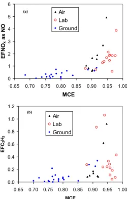
observed in the airborne and lab studies, which were at higher average MCE. This in-dicates that, for these smoldering compounds, the fuel difference associated with these different platforms did not eliminate the basic tendency for higher EF at lower MCE. A reversed pattern is shown for flaming compounds in Fig. 3a (NO_x) and 3b (C₂H₂). Again

5

the EF depend mainly on the amount of flaming and smoldering combustion. The one low NOx point at high MCE was for dambo grass, which had very low fuel nitrogen

(Table 1). For these four compounds (and in general), the few ground-based samples with MCE that was high enough to overlap the MCE observed in the other studies have EF that fit in remarkably well. The lowest MCE fire from the lab study (Ps, Tables 1

10

and 3) had EF that seemed to be possible outliers when looking only at the lab data, but these EF fit well into the full range established by the other studies (Figs. 2 and 3). Also apparent, in the methanol plot (Fig. 2b), is the excellent agreement between the open-path FTIR and the PTR-MS for this compound.

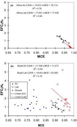
Our combined TROFFEE data also reveal a few compounds that previously showed

15

strong negative correlation with MCE (classic “smoldering compounds”) for which the negative correlation is weakened or absent in the TROFFEE “coupled” data set. A good example of this is C2H4. First, in Fig. 4a, we show the highly-correlated EFC2H4 vs.

MCE for airborne and lab samples of African savanna fires from Yokelson et al. (2003) and Christian et al. (2003). Then Fig. 4b shows all the TROFFEE C₂H₄data. In Fig. 4b

20

there is still good agreement between the three platforms in the MCE range where they overlap (MCE∼0.9), but there is not a strong indication that the average EF at low MCE is higher than the average EF at high MCE. Thus, the classic smoldering compound pattern breaks down, even though the pattern is apparent when only the lab, or only the airborne data, is considered. One possible explanation is that the smoldering logs

25

sampled in the ground-based study (and to a lesser extent in the airborne study) emit less C2H4per unit mass than smoldering foliar fuels. Another possibility is that C2H4is

produced by both direct pyrolysis of biomass and incomplete oxidation in flames as may also be the case for C₂H₂. Another compound which may belong in this inconclusive

(15)

ACPD

8, 4221–4266, 2008

Full Screen / Esc

Interactive Discussion category is HCHO.

Finally, a few compounds have little correlation with MCE in both this and earlier work. Chief among these are HCN (Fig. 4c), acetonitrile (Fig. 4d), and formic acid. The lack of a strong dependence on MCE can aid in the use of HCN and acetonitrile as biomass burning tracers. Specifically, knowing the MCE of the fire source is not

5

that important (as opposed to the case when using K). However, the EF for HCN and acetonitrile are quite variable for tropical forest fires and significantly different, highly variable emissions of these compounds are produced by other global types of biomass burning. This may be related to fuel nitrogen differences (Yokelson et al., 2007a, b).

In theory, capturing our full measured range of EF versus MCE would significantly

10

enhance the accuracy of emissions estimates and the input for local-global models. For instance, the average EFCH4 varies by about a factor of 20 over the MCE range

sampled during TROFFEE. Unfortunately, the prospects for measuring the MCE of fires from space as they occur are not good as it would require very accurate quantification of small CO2 enhancements against a large background and a very precise spatial

15

scale. We cannot even be confident of seasonal trends in average MCE for fires in the major, global biomass burning areas for reasons discussed in Yokelson et al. (2007a), Korontzi et al. (2003), and Hoffa et al. (1999). For example, in TROFFEE we have evi-dence that the MCE of lofted plumes seems to increase as the dry season progresses, but we suspect that the amount of low-MCE residual smoldering combustion may also

20

increase as the large diameter fuels dry out (Yokelson et al., 2007a). Thus, for now, we attempt to estimate one MCE and a set of associated EF for all the detected emissions that are intended for application to the whole dry season. We provide this for the two main types of fires in the Brazilian Amazon: primary deforestation fires and pasture maintenance fires – each of which are thought to consume about 240 Tg of biomass

25

annually in the region (Yokelson et al., 2007a). We hypothesize that our EF for Brazil are also reasonable for these fire types in the other tropical forests around the globe. However, we note that pasture fires are thought to be far less significant relative to primary deforestation fires in the other major tropical forest areas of the globe.

(16)

ACPD

8, 4221–4266, 2008

Full Screen / Esc

Interactive Discussion Our derivation of recommended EF values draws on ground-based measurements

of the amount of fuel consumed by the plume-forming and residual-smoldering stages of real fires in Brazil. As discussed in detail by Christian et al. (2007) and references therein, the available evidence suggests that for tropical deforestation fires about 5% of the fuel is consumed by residual smoldering and 95% is consumed during the

convec-5

tive plume forming phase of the fire. On the other hand, for pasture maintenance fires, it seems likely that about 40% of the fuel is consumed by residual smoldering with the balance (60%) feeding into the initially-lofted emissions. Thus, for the 14 compounds for which we have both airborne and ground-based EF for real fires in Brazil, we simply take an average of the airborne and ground-based EF weighted according to the above

10

percentages. (An explicit formula for this straightforward process has been given else-where (Bertschi et al., 2003a; Christian et al., 2007)). The one pasture fire sampled from the air had lofted emissions that were not significantly different (statistically) than the other fires so we used the study-average airborne values for both fire types. Table 4 shows the EF for deforestation and pasture maintenance fires calculated in this way.

15

One important result of this approach is that the average fire-integrated MCE for pri-mary deforestation fire is calculated to be 0.904 and the average fire-integrated MCE for pasture fires is 0.861.

Because no ground-based sampling of fires was done in TROFFEE with filters, PTR-MS, or GC, there are 27 compounds and PM for which we have EF measurements

20

only from the air and lab. For these compounds we need a method to start with lab and/or airborne data and derive EF that represent the total emissions from authentic primary deforestation and pasture fires. Several approaches were tested by applying them to the compounds for which we had both ground and airborne field data and then calculating how well the predictions agreed with the values obtained as described

25

above. For instance, Christian et al. (2003) found that using the lab-based EF vs. MCE equation at the field-average MCE returned EF that agreed well with the field average EF for savanna fires. However, for TROFFEE, the lab equations tended to significantly overpredict the field measured EF (factor of ∼2 on average). After adding a correction

(17)

ACPD

8, 4221–4266, 2008

Full Screen / Esc

Interactive Discussion for the average bias, using the airborne EF vs. MCE relation to calculate EF at the

MCE for deforestation and pasture fires worked well for some compounds, but not for others (e.g. formaldehyde and acetic acid) and the typical error was 65–70% of the target value. Predictions with smaller error (averaging 10–40% of the target) were eventually obtained from a simpler approach. We found that for smoldering compounds

5

not containing nitrogen the following relations were observed:

EF (for primary deforestation fires) = EF (airborne average) × 1.12 ± 0.11 (2) EF (for pasture maintenance fires) = EF (airborne average) × 2.00 ± 0.90 (3) Equation (2) suggests that a 12% increase of the airborne average EF for smoldering compounds is appropriate for primary deforestation fires, which seems not too

contro-10

versial as this involves a small increase to compensate for a small amount of unsam-pled smoldering emissions. Equation (3) makes the bolder suggestion that the average airborne EF (for smoldering compounds) should be doubled to obtain a fire-integrated value appropriate for pasture fires. This prediction is close for some of the “standard” compounds (e.g. CH₄, 1.81; C₃H₆, 1.87; CH₃OH, 2.21). However, it’s further off for

15

other compounds such as HCOOH (0.89), CH3COOH (2.90), furan (3.14), and phenol

(3.41). Thus, estimates for pasture fires based on this formula have considerable un-certainty, but are probably a step in the right direction for most compounds. The EF estimated using Eqs. (2) and (3) are shown as a second group of EF in Table 4.

The predictions for pasture fires based on Eq. (3) are perhaps most intriguing for

20

particles. The airborne average for PM₁₀ was 17.8±4.1. This EF was already larger than values obtained in previous studies as discussed by Yokelson et al. (2007a): pos-sibly due partly to a trend toward larger fires in the Amazon. Doubling this value, as suggested by Eq. (3), to obtain an EF for pasture fires, then implies a fire-integrated EFPM10 of 35.6 g/kg, which is well above the range usually recommended for various

25

types of biomass burning (Andreae and Merlet, 2001). Alternate methods to estimate an EF for PM at the pasture fire MCE of 0.861 can also be tried. For instance, using the EF versus MCE relationship from the airborne data returns an EFPM of 23.4 g/kg

(18)

ACPD

8, 4221–4266, 2008

Full Screen / Esc

Interactive Discussion at the pasture fire MCE of 0.861. On the other hand, using the lab based EF vs. MCE

for PM2.5 returns a pasture fire EFPM2.5 of 27.1 g/kg. If this EFPM2.5 is increased by

20% to account for the typical difference between PM2.5and PM10(Artaxo et al., 1998;

Andreae and Merlet, 2001) we obtain an EFPM₁₀ of 33.9 g/kg, which agrees remark-ably well with the prediction of Eq. (3). At this point it is worth noting that our airborne

5

PM10 measurements by nephelometer are reasonably consistent with our lab-based

gravimetric measurements of PM_2.5as shown in Fig. 5.

We also have gravimetric EFPM2.5measurements for temperate-forest woody

mate-rials from previous laboratory experiments that are relevant to this discussion. Christian et al. (2003) reported two gravimetric spot-measurements of a smoldering (hardwood)

10

cottonwood log in their Table 2. The EFPM_2.5 for one Teflon filter was 20.9 g/kg. A second (quartz filter) sample showed 24.48 gC/kg. Since biomass burning particles are typically 60% C, this second sample could imply the “spot” EFPM2.5 was 41 g/kg.

Bertschi et al. (2003a) made 12 gravimetric spot-measurements of the “instantaneous” EFPM2.5 during a lab fire that burned first a woody (softwood) stump and then duff

15

and organic soil (Fig. 6). The stump was ignited on top and the first 6 filter samples taken reflected consumption of the stump. The EFPM_2.5for these samples ranged from 20.5–109 g/kg with an average (weighted by the fuel consumption data) of 30.6 g/kg. (The EFPM2.5 for smoldering duff was only 2.95 g/kg and the fire average reported

by Bertschi et al. was 15.8 g/kg.) If we increment the average EFPM_2.5 for the stump

20

by 20% we obtain an EFPM10 for unlofted smoldering of woody material of 38.3 g/kg.

Taking 40% of this value and 60% of the airborne average of 17.8 g/kg yields a fire-integrated EFPM₁₀ for pasture fires of 26.0 g/kg. This last value agrees reasonably well with the EFPM10 obtained at the pasture fire MCE from the airborne PM10

mea-surements (23.4 g/kg). Thus, we take 23.4 g/kg and 18.7 g/kg (80% of the PM10) as

25

conservative estimates for EFPM₁₀ and EFPM_2.5 for pasture fires, respectively. The analogous values for primary deforestation fires would be 18.5 and 14.8 g/kg.

Several summary statements are in order. In general, our TROFFEE EFPM are higher than in previous studies (9–11 g/kg PM_2.5, Ferek et al., 1998; Andreae and

(19)

ACPD

8, 4221–4266, 2008

Full Screen / Esc

Interactive Discussion Merlet, 2001). This implies that much more primary particulate matter is produced by

tropical deforestation than previously assumed. For example, assuming equal amounts of biomass consumption by primary deforestation fires and pasture maintenance fires (Kauffman et al., 1998), we obtain an Amazon-average EFPM2.5 of 16.8 g/kg. This

implies about 85% more PM_2.5 emissions from the region than using the Andreae

5

and Merlet (2001) recommendation of 9.1 g/kg. The physical basis for this increase is the inclusion of a larger contribution from smoldering combustion. The impact of this increase may be partially offset by any tendency for some of the initially unlofted particles to have a shorter atmospheric lifetime. Also, our evidence for this increase is far from conclusive, but not without merit. Thus, more measurements would be

10

valuable. Finally, though pasture fires and deforestation fires are thought to consume roughly equal amounts of biomass in the Brazilian Amazon (Kauffman et al., 1998), pasture fires likely produce more of the particle and trace gas pollutants. However, the average fuel consumption on primary deforestation fires could be increasing due to an increase in land conversion to mechanized agriculture (Christian et al., 2007).

15

There are three compounds that were measured only in the lab fires: glycolalde-hyde, propanenitrile, and methylvinylether. Methylvinylether was detected by FTIR in only one lab fire and thus, we point out that it is emitted in trace amounts, but can’t give a numerical recommendation. For the two other compounds, we estimate the emis-sions from field fires using the lab-measured ratio of the compound to the most similar

20

species that was measured in the field. Specifically the lab ratio of propanenitrile to acrylonitrile (2.1) times the field acrylonitrile gives the estimate for propanenitrile for the field fires. (Acrylonitrile is also known as propenenitrile.) Similarly, the lab ratio glycolaldehyde/acetic acid (0.31) times the field acetic acid gives our estimates for field glycolaldehyde.

25

The final category of compounds to address is those that were measured only in the airborne canister sample of one above-average MCE fire (Yokelson et al., 2007a). We don’t have information on the MCE dependence of these compounds nor can we make an estimate of variability. We simply report our one measurement in Table 4.

(20)

ACPD

8, 4221–4266, 2008

Full Screen / Esc

Interactive Discussion We next compare the amount of emissions data available for tropical deforestation

fires to other types of global biomass burning. In TROFFEE we had filters, OP-FTIR, and GC-PTR-MS in the lab, and PTR-MS, FTIR, and whole air sampling (WAS) in the field followed by GC analysis. Thus, we now have more complete emissions data for tropical forest fires than for any other type of global biomass burning. Significant

im-5

provements for the tropical forest fire data base could be realized by having more WAS in the air and gravimetric and PTR-MS measurements on the ground and by having GC-PTR-MS in the field to remeasure the branching ratios for selected masses. The next best data is available for savanna, peat, and agricultural waste fires. These fires have been studied with WAS, FTIR, and lab-fire PTR-MS, but not with GC-PTR-MS

10

and with only minimal field use of PTR-MS. Many additional field measurements of the smoke from agricultural waste fires involving WAS and FTIR were recently completed in Mexico (Yokelson et al., 2007b) and this database should improve significantly in the near future. Finally, for cooking fires and boreal forest fires the existing field measure-ments are almost exclusively by WAS and FTIR and neither PTR-MS nor extensive lab

15

measurements have been carried out. In April-May of 2007 a large number of cooking fires were sampled in Mexico with FTIR and filters, and this will provide more exten-sive trace gas data and the first field-measured EFPM for these fires (Christian et al., 20081).

3.3 Characteristics of biogenic and pyrogenic sources: Amazon to global

20

In the TROFFEE experiment we focused on the pyrogenic and biogenic emissions from the Amazon basin. In this section we present rough estimates of the magni-tude of these sources at various scales to explore their role in atmospheric chemistry. We start at the local scale noting that Karl et al. (2007b) measured average isoprene

1

Christian, T. J., Yokelson, R. J., Alvarado, E. C., et al.: Emissions from cooking fires, garbage burning, brick making, and other biomass burning sources in central Mexico, Atmos. Chem. Phys. Discuss., MILAGRO special issue, in preparation, 2008.

(21)

ACPD

8, 4221–4266, 2008

Full Screen / Esc

Interactive Discussion emissions from pristine tropical forest of ∼400±130 g/ha day. This can be compared

to the affect of burning a hectare of tropical forest (which typically requires less than one day) assuming a fuel consumption of ∼120±40 Mg/ha (Christian et al., 2007) and our primary deforestation EF for isoprene from Table 4 (0.42±0.13 g/kg). The burned hectare releases a pulse of ∼50 000±23 000 g of isoprene, which is >120 days of

pro-5

duction by an unburned hectare. However, only a small percentage of the Amazon basin burns every year (∼2.5%) so we expect the emissions from plants to dominate the annual basin-wide isoprene budget. Explicitly, assuming four million km2of tropical forest in the Amazon basin (Yokelson et al., 2007a) implies an annual biogenic iso-prene source of ∼58±19 Tg. (The uncertainty quoted in the biogenic source does not

10

include the uncertainty in forest area in this and the following estimates.) Approximately 2.0±0.5 million ha of the Amazon are subjected to primary deforestation fires annu-ally (http://www.obt.inpe.br/prodes/), which suggests that these fires consume about 2.4±1. 0×1011kg/yr of fuel. Kauffman et al. (1998) calculated that pasture fires in the Amazon basin consume roughly the same amount of biomass as primary deforestation

15

fires. We combine the fuel consumption for these fire types with the EF for isoprene for these fire types from Table 4 and obtain an annual pyrogenic isoprene source of 0.28±0.16 Tg (∼0.5% of biogenic source).

Analogous basin-wide annual estimates can be made for other individual NMOC emitted by both sources. For instance, the methanol to isoprene emission ratio for

20

tropical forests was measured at 14% in Costa Rica (Karl et al., 2004) and 4% dur-ing TROFFEE (Karl et al., 2007b). Takdur-ing an average value of 9±5% then implies an annual methanol source of ∼5.3±3.4 Tg from intact Amazonian forest. Using the fuel consumption estimates above and the EF for methanol from Table 4 yields an an-nual Amazon-basin pyrogenic source of methanol of ∼2.1±1.1 Tg. In this case the fire

25

source is about 40% of the plant source on an annual basis and the two sources would be comparable during the dry season.

Significant biogenic emissions of acetaldehyde, acetone, and monoterpenes have also been quantified from tropical forest. Taken together, Karl et al. (2004, 2007b) imply

(22)

ACPD

8, 4221–4266, 2008

Full Screen / Esc

Interactive Discussion that the sum of quantified non-isoprene emissions from tropical forest equals about

35±9% of isoprene. Increasing our estimate of isoprene emissions (58 Tg) by 35% implies emissions of 79±33 Tg/yr of “known” NMOC from the Amazon basin. Using the sum of measured pyrogenic NMOC from Table 4 (∼26 or ∼48 g/kg for forest or pasture fires, respectively) yields a pyrogenic source of known NMOC from the Amazon basin

5

of ∼18±11 Tg/yr. The pyrogenic NMOC are about one-quarter of the biogenic NMOC in this case. Next, we note that the total mass of NMOC emitted by fires is actually about twice the measured mass of NMOC (see Sect. 2.4.) and the ratio of total/known, non-isoprene NMOC for plants could be similar (Goldstein and Galbally, 2007). If we double both the pyrogenic NMOC and the non-isoprene biogenic NMOC, we estimate the

10

annual Amazonian pyrogenic and biogenic total NMOC at about 35±20 and 99±53 Tg, respectively.

Fires also emit a substantial amount of methane (a VOC) and CO, which is some-times used as a proxy for VOC (or a pseudo-VOC) in simpler global models (Crutzen and Carmichael, 1993). If we add CO and CH4(using Table 4 as above) to the

pyro-15

genic NMOC emissions, which are also VOC, the Amazonian, known “pyrogenic VOC” are about 84±42 Tg/yr – or roughly equal to the known biogenic VOC (ignoring non-foliar forest methane sources). But we note that the biogenic emissions have higher OH rate coefficients on average and dominate the regional OH reactivity (Karl et al., 2007b).

20

We can also compare the impact of these two sources on the regional carbon cycle (although other processes such as photosynthesis, respiration, metabolism in soils, river outgassing, etc. are critical in a full C cycle treatment (Chou et al., 2002; Lloyd et al., 2007)). We multiply the total biogenic emissions (99 Tg including estimated unknown NMOC) by 60/68 (the mass ratio of C to total mass in isoprene) to roughly

25

estimate that the plant emissions include about 87±46 Tg C/yr. Assuming the biomass consumed by regional fires is 50% C and that all this C enters the atmosphere suggests that the total carbon added to the atmosphere by these fires is ∼240±100 Tg C/yr. The biogenic “C as NMOC” added to the atmosphere by pristine forest is almost 40% as

(23)

ACPD

8, 4221–4266, 2008

Full Screen / Esc

Interactive Discussion large as the C added by the fires used to remove forest material.

The annual Amazonian fire initial emissions of PM2.5from Table 4 are about 8±5 Tg.

Reid et al. (1998) reported that Amazonian primary pyrogenic fine-mode aerosol in-creased in mass by a factor of 1.8 during the first 1–3 days after emission due to secondary processes involving mostly co-emitted pyrogenic trace gases. If we

as-5

sume for illustrative purposes that the co-emitted inorganic, pyrogenic species such as NO_x, NH₃, and SO₂(Table 4) were 100% converted to aerosol nitrate, ammonium, and sulfate; then about 2.4 Tg of the total regional mass growth in PM2.5 (∼6.4 Tg)

could be due to these species. Thus, the inorganic species would account for ∼38% of the mass growth and about 62% (4 Tg) would be due to co-emitted pyrogenic NMOC.

10

This implies that less than ∼11% of the co-emitted pyrogenic NMOC (35 Tg) would have oxidized and/or condensed on the fine particles (during 1–3 days) since we are ignoring changes in NMOC mass during oxidation. It’s also likely that some of the secondary organic aerosol (SOA) would have come from the biogenic NMOC, which are more abundant regionally although less concentrated in initial plumes. A biogenic

15

component to the Amazonian, moderately-aged, dry-season, fine-mode aerosol was not observed (or ruled out) by Echalar et al. (1998) even though they clearly measured a large biogenic contribution to the coarse-mode, dry-season aerosol (diameter >2 microns). They also observed large biogenic components to both modes in the wet season. In any case, the total regional PM mass growth (6.4 Tg) implied by the mass

20

growth factor measured by Reid et al. (1998) is equivalent to only ∼7.5% of our es-timated total mass of NMOC emitted during the Amazonian dry-season by pyrogenic and biogenic sources together (assuming dry season equals one-half annual for bio-genics). The estimated organic part of the regional mass growth (4 Tg) is less than 5% of the total regional NMOC. Thus, over the time scale of several days, 5% represents a

25

rough upper limit on the percentage conversion via SOA for regional NMOC. This upper limit is consistent with the lower end of estimates of the fraction of biogenic emissions converted to PM by secondary processes, which range from ∼3 to ∼66% (Andreae and Crutzen, 1997; Goldstein and Galbally, 2007). Clearly the percent conversion for

(24)

indi-ACPD

8, 4221–4266, 2008

Full Screen / Esc

Interactive Discussion vidual NMOC varies greatly and more measurements are needed to support a rigorous

overall accounting.

In light of the above budgets, it seems unlikely that 66% of the Amazonian biogenic NMOC condense on the Amazonian pyrogenic fine particles within 1–3 days of aging as might be inferred from Goldstein and Galbally (2007). A percentage conversion that

5

high would represent a mass growth factor of >8.2. No Amazonian field measurements support a growth factor this large at this time to our knowledge. Conversely, if 66% of biogenic NMOC did convert to secondary organic aerosol, then tropical forest regions would be producing well over ten times more fine particle mass than is currently in-cluded in conventional inventories of primary aerosol.

10

Further, the amount of regional SOA formation is constrained somewhat by source apportionment studies of the total aerosol mass in the Amazon dry season. Artaxo et al. (1998) made airborne measurements of aerosol characteristics in approximately the same regional haze investigated by Reid et al. (1998) during SCAR B. They ob-served an average regional mass of total aerosol of 107 µg/m3of which 78% was in the

15

fine mode. These authors also performed source apportionment for the total aerosol mass and obtained a ratio for the biogenic/pyrogenic components of 34.6%. Guyon et al. (2004) measured the average ratio for the biogenic/pyrogenic component of total aerosol mass as 35.5% in a tower-based study conducted during the Amazonian dry season. We can couple this with a rough estimate of the upper limit for the total

pyro-20

genic, regional, dry-season, aerosol mass by multiplying our regional pyrogenic PM10

(10 Tg, Table 4) by 1.8 to obtain 18 Tg. (A growth factor this large for pyrogenic PM10

has not actually been measured.) If the biogenic component is 35% of 18 Tg, that im-plies a regional, dry-season, biogenic total aerosol mass of 6.3 Tg. This last value is ∼12% of the regional, dry-season, biogenic NMOC production of ∼50 Tg. Thus, 12%

25

would be a large overestimate of the percentage conversion by SOA as we are ignor-ing a large biogenic component to the primary total aerosol mass and mass changes during oxidation. In summary, only ∼5% of the regional NMOC seem to be converted to aerosol within the Amazonian boundary layer on the time scale of 1–3 days.

(25)

How-ACPD

8, 4221–4266, 2008

Full Screen / Esc

Interactive Discussion ever, a larger percentage could convert to SOA on longer time scales and/or outside

of the Amazonian boundary layer. This could involve NMOC with lifetimes greater than several days and/or NMOC with shorter lifetimes that experience rapid transport to the free troposphere (Heald et al., 2005; Andreae et al., 2001).

Next we roughly characterize the total NMOC emissions from fires and plants at

5

the global scale. We start by deriving a best estimate of global isoprene emissions from vegetation of 600 (range 500–750) Tg/yr using the MEGAN model (Guenther et al., 2006). Using the same assumptions as above for both non-isoprene and un-known NMOC suggests a global biogenic NMOC source of ∼1000 Tg/yr (range 770– 1400 Tg/yr).

10

Our global, pyrogenic, NMOC estimate is derived in some detail. Coupling the sum of our EFNMOC for deforestation fires (Table 4) with an estimate of biomass consump-tion in global deforestaconsump-tion fires (1330 Tg/yr, Andreae and Merlet, 2001 (uncertainty not provided, but large)) implies that global deforestation fires produce over 34 Tg/yr of identified NMOC. We are not considering the higher emissions from pasture

main-15

tenance fires in our global estimate. Our estimate does include the 12% increase we applied to our airborne EF for primary deforestation fires to account for residual smol-dering combustion. Since we only measured about one-half the NMOC on a mass basis (Sect. 2.4), then the total annual NMOC from global deforestation fires should be about 69 Tg/yr. This estimate and an analogous estimate for each main type of

20

biomass burning listed by Andreae and Merlet (2001) are shown in Table 5. In Table 5, we have shown the biomass consumption by each type of burning, the total NMOC cur-rently quantified for that type of burning, and we assume that real total NMOC are twice the measured total NMOC. This last assumption is conservative since the instrumen-tation required to measure half the NMOC was only available for tropical forest fires (in

25

this work). In fact, for the category of biomass burning that produces the most global NMOC (cooking fires) only FTIR was available. The real conversion from measured to total NMOC for cooking fires could be closer to three. Also, as part of TROFFEE, Christian et al. (2007) reported a sum of NMOC measured by FTIR from burning dung

(26)

ACPD

8, 4221–4266, 2008

Full Screen / Esc

Interactive Discussion (an important cooking fuel in China and India) that was 32% higher than the value we

use (for wood cooking fires) in Table 5. The last column of Table 5 shows our estimate of total annual NMOC by type of fire and a conservative global sum of 466 Tg/yr. For reasons given just above, the real global sum is probably over 500 Tg/yr. Its worth noting that this global pyrogenic NMOC estimate is much larger than the ∼100 Tg/yr

5

estimated earlier by Andreae and Merlet (2001). There are sound reasons for this increase. Mainly: (1) subsequent development of methods (FTIR, PTR-MS, and GC-PTR-MS) to quantify the previously poorly-characterized emissions of reactive OVOC, that account for ∼80% of the NMOC in biomass burning smoke, (2) deployment of the new instrumentation on previously undersampled burning types such as cooking fires,

10

charcoal kilns, agricultural waste, etc., and (3) the capability of PTR-MS to estimate the unknown NMOC.

In light of our updated estimate, biomass burning is easily the second largest source of global NMOC behind plants (∼1000 Tg/yr, see above) and well ahead of anthro-pogenic sources (142 Tg “C as NMOC”/yr, Middleton, 1995). Biomass burning has

15

already long been recognized as the largest global source of primary fine carbona-ceous particles (50–190 Tg/yr, diameter <1 micron, Kreidenweis et al., 1999 (see their Table 4.1)). In addition, the ∼500 Tg/yr of NMOC from biomass burning should proba-bly be added to the ∼1000 Tg/yr of NMOC from vegetation as major global sources of secondary organic aerosol.

20

Finally, it is a fair approximation to assume that biogenic NMOC emissions are given off in diffuse manner according to a predictable daily cycle that should be fairly straight forward to implement in local-global models. On the other hand, fire emissions are pro-duced in concentrated pulses and undergo significant initial processing in an altered chemical regime whose best depiction in local-global models is still unknown

(Trent-25

(27)

ACPD

8, 4221–4266, 2008

Full Screen / Esc

Interactive Discussion 3.4 Sugar cane

In many heavily populated areas of the tropics and subtropics large areas of sugar cane are burned, which can add to regional air quality concerns (Lara et al., 2005; Canc¸ado et al., 2006). Top sugar producing areas (2004 data) in order are: southern Brazil, India, China, Thailand, Pakistan, Mexico, Colombia, Australia, Philippines, southern

5

US (including Hawaii), Indonesia, and Cuba. (http://www.fao.org/statistics/yearbook/

vol 1 1/pdf/b08.pdf). The most common sugar cane varieties take two years to mature. In this time, dried leaves and weeds accumulate and the most economical method of separating them from the cane is to burn the field just before harvest. This also eliminates pests that can hinder manual harvesting. About 20 Mg/ha of biomass is

10

consumed in these fires and Brazil alone has about 4.5 million ha planted in sugar cane with over half of these hectares in densely populated S ˜ao Paulo State (Lara et al., 2005). There are sugar cane varieties that don’t require burning before harvest, but there are barriers to adopting these varieties: lower yield, less economical, and potential job loss (over a million workers are employed by the traditional sugar cane

15

industry in Brazil alone (Lara et al., 2005)).

Only a few studies exist on the initial particle and trace gas emissions from burning sugar cane and their influence on the atmosphere. These studies were in S ˜ao Paulo State, Brazil, where over 50% of the world’s sugar cane is produced (Yevich and Logan, 2003). At a sampling site about 4 km from downtown Piracicaba (population ∼320 000)

20

and 1 km from a sugar cane plantation, sugar cane burning contributed 60% of annual PM_2.5. In the same city, particle emissions from sugar cane fires were associated with increased hospital visits for respiratory problems by children and elderly patients (Canc¸ado et al., 2006). Table 3 gives our EFPM2.5for sugar cane burning as 2.17 g/kg.

However, this value, while accurate, is from a single laboratory fire that burned at an

25

MCE that is higher than normally obtained in the field for biomass burning. We have no field measurements to indicate the MCE of a typical sugar cane fire, but it is likely lower and that would imply a larger EFPM_2.5 (e.g. see Fig. 5). Since emission ratios

(28)

ACPD

8, 4221–4266, 2008

Full Screen / Esc

Interactive Discussion to CO normally vary less strongly with MCE than do EF, it is of value to also express

our PM2.5 data in this way. On a mass basis PM2.5/CO is 0.077, which is equivalent to

88 µg/m3 per ppm of CO. These ratios are well within the “normal range” for biomass burning.

To our knowledge, the only previously published measurements of gas-phase

emis-5

sions from sugar cane burning are by da Rocha et al. (2003). They used NaOH-impregnated cellulose filters to measure gaseous acidic species (formic acid, acetic acid, HCl, HNO3, and SO2) only 1–2 m from a sugar cane fire near the city of

Araraquara. These authors report a molar emission ratio of formic to acetic acid of 2.95. In contrast, we find that acetic acid is the dominant organic acid (acetic/formic

10

= 5.72, or formic/acetic = 0.175). Thus our acetic/formic ratio is 17 times higher, but neither study is extensive enough to fully assess natural variation in this ratio. Whereas Lara et al. (2005) found that ambient PM_2.5increased during the cane burning season, da Rocha et al obtained results for ambient gases that are harder to rationalize. Their ambient formic and acetic levels decreased during the burning season even though

15

they are major biomass burning products. On the other hand, minor burning products such as HCl, SO2, and HNO3increased by 100–300% during the burning season.

Bagasse is the residual, fibrous biomass left behind after milling (compressing) the cane. It can be used for animal feed and in the manufacture of paper, but it is also burned to produce electricity and represents a second, as yet uncharacterized,

emis-20

sions source for sugar cane. Also, though sugar cane and bagasse burning together account for only a small fraction of the total annual biomass burned on a global scale, sugar cane fields are typically located closer to urban or semi-urban areas and thus burning sugar cane may have a larger relative health impact.

4 Conclusions

25

Detailed measurements were made of the emissions from laboratory fires burning trop-ical forest fuels as part of the Troptrop-ical Forest and Fire Emissions Experiment

(29)

(TROF-ACPD

8, 4221–4266, 2008

Full Screen / Esc

Interactive Discussion FEE). In most cases, about one-third of the fuel chlorine ended up in the particles and

about one-half in the ash. About 50% of the total mass of volatile NMOC emitted by these fires could be identified. The lab fire emission factors (EF) were integrated with EF obtained during the TROFFEE airborne and ground-based field campaigns, and with field measurements of fuel consumption. This procedure produced recommended

5

EF for all measured species for both primary deforestation fires and pasture main-tenance fires. Most of the NMOC and particle EF are 20–80% larger than previously suggested; mostly because our new method includes a significant contribution from the recently-measured, initially-unlofted smoldering emissions. The TROFFEE EFPM2.5is

14.8 g/kg for primary deforestation fires and 18.7 g/kg for pasture maintenance fires.

10

These EF imply a pyrogenic PM_2.5 source for the Amazon that is 84% larger than a widely-used previous recommendation for tropical deforestation EFPM2.5 (9.1 g/kg).

Plants are the main source of isoprene in the Amazon basin, but much larger iso-prene concentrations can be generated in smoke plumes. Even though plants are the main global source of methanol, fire can be a comparable source of methanol in

15

the Amazon basin during the dry season. More total NMOC are emitted by plants and they dominate the OH reactivity of the region, but fires contribute a compara-ble amount of total VOC. Coupling source apportionment studies and observations of secondary aerosol formation in the Amazon with our regional trace gas and PM2.5

bud-gets for the dry season suggests that about 5% of the total mass of pyrogenic and

20

biogenic NMOC contribute to secondary aerosol formation within the regional bound-ary layer on a time scale of 1–3 days. A conservative estimate of global pyrogenic NMOC is ∼466 Tg/yr, which clearly establishes biomass burning as the second largest global source of NMOC (after plants) and a potential major global source of secondary aerosol. A few emission ratios (ER) appropriate for sugar cane burning were also

25

measured, which may help estimate the air quality impacts of burning this major crop.

Acknowledgements. This research was supported primarily by NSF grant ATM0228003.

R. J. Yokelson was also supported by the Interagency Joint Fire Science Program, the Rocky Mountain Research Station, Forest Service, U.S. Department of Agriculture (agreements