HAL Id: hal-01982982
https://hal.archives-ouvertes.fr/hal-01982982
Submitted on 16 Jan 2019
HAL is a multi-disciplinary open access
archive for the deposit and dissemination of
sci-entific research documents, whether they are
pub-lished or not. The documents may come from
teaching and research institutions in France or
abroad, or from public or private research centers.
L’archive ouverte pluridisciplinaire HAL, est
destinée au dépôt et à la diffusion de documents
scientifiques de niveau recherche, publiés ou non,
émanant des établissements d’enseignement et de
recherche français ou étrangers, des laboratoires
publics ou privés.
2050
Sebastien Bourdarie, Alexandre Fournier, Angélica Sicard, Gauthier Hulot,
Julien Aubert, Denis Standarovski, Robert Ecoffet
To cite this version:
Sebastien Bourdarie, Alexandre Fournier, Angélica Sicard, Gauthier Hulot, Julien Aubert, et al..
Impact of the Earth’s magnetic field secular drift on the low altitude proton radiation belt from years
1900 to 2050. RADECS 2018, Sep 2018, GOTEBORG, Sweden. �hal-01982982�
Abstract—The effects of the space radiation environment on
spacecraft systems and instruments are significant design considerations for space missions. In order to meet these challenges and have reliable, cost-effective designs, the radiation environment must be understood and accurately modeled. The low altitude proton environment varies slowly in time due to the secular drift of the Earth’s main magnetic field and due to the evolution of the solar cycle. The purpose of this paper is to extend the OPAL model [1] capabilities by introducing a prediction of the Earth’s main magnetic field model up to year 2050. Impact on low altitude spacecraft radiation specification for next space missions is then assessed.
Index Terms—radiation belts, trapped protons, South Atlantic
Anomaly forecast
I. INTRODUCTION
Specification of the high-energy radiation belt proton environment remains an outstanding issue for both present and future low altitude spacecraft design and analyses. In 2014, the OPAL model dedicated to altitudes below 800 km was issued to describe the > 80 MeV trapped protons in the Earth’s radiation belts [1]. The model accounts for the secular drift of the Earth’s main magnetic field based on IGRF and NOAA data from 1980 to 2012 and for the solar cycle modulation impact of the proton flux.
In the present study we extend the capabilities of the OPAL model by accounting for both the full IGRF-12 model between 1900 and 2015, and the predicted evolution of the Earth’s main field up to 2050. We first describe the magnetic field models being used and the way the main field is being forecasted up to 2050 (section II). We next describe the methodology used to characterize the evolution of the low altitude proton radiation belt, comparing these updated OPAL predictions to those of the AP8min model [2], and discuss this evolution, illustrating its impact on spacecraft specification
This work was supported by Grants 4500055251/
DIA094, which is part of CNES R&T program (R-S17 / MT-0003-187). S. Bourdarie and A. Sicard are with ONERA / DPHY, Université de Toulouse, F-31055 Toulouse – France, (e-mail:
A. Fournier G. Hulot and J. Aubert are with IPGP, Sorbonne Paris Cité, Université Paris Diderot, UMR 7154 CNRS/INSU, F-75238 Paris – France.
D. Standarovski and R. Ecoffet are with CNES, F-31401 Toulouse, France.
(section III) and finally conclude (section IV).
II. THE EARTH’S INTERNAL MAGNETIC FIELD
The Earth’s internal magnetic field is known to vary slowly in time. The typical time scale is on the order of months and longer: this is the so-called secular variation.
Consequently, the Earth’s main field is defined in terms of a
sequence of time-dependent Gauss coefficients 𝑔𝑔𝑙𝑙𝑚𝑚(𝑡𝑡) and
ℎ𝑙𝑙𝑚𝑚(𝑡𝑡), such that the magnetic potential V in a source-free
region reads
𝑉𝑉(𝑟𝑟, 𝜃𝜃, 𝜑𝜑, 𝑡𝑡) = 𝑎𝑎 ∑𝑙𝑙=𝐿𝐿𝑙𝑙=1𝑇𝑇∑𝑚𝑚=𝑙𝑙𝑚𝑚=0�𝑎𝑎𝑟𝑟�𝑙𝑙+1[𝑔𝑔𝑙𝑙𝑚𝑚(𝑡𝑡) cos 𝑚𝑚𝜑𝜑 +
ℎ𝑙𝑙𝑚𝑚(𝑡𝑡) sin 𝑚𝑚𝜑𝜑] 𝑃𝑃𝑙𝑙𝑚𝑚(𝑐𝑐𝑐𝑐𝑐𝑐𝜃𝜃),
in which (r,θ,φ) are spherical coordinates, t is time, a=6371.2
km is the average radius of the Earth, and 𝑃𝑃𝑙𝑙𝑚𝑚 represents the
Schmidt quasi-normalized associated Legendre functions of
degree l and order m. LT is the truncation of the spherical
harmonic expansion. The 𝑔𝑔𝑙𝑙𝑚𝑚and ℎ𝑙𝑙𝑚𝑚 are expressed in nT. The International Association of Geomagnetism and
Aeronomy (IAGA) released the 12th Generation International
Geomagnetic Reference Field (IGRF-12) in December 2014 [3]. It provides Gauss coefficients for years from 1900 to 2010 with a five years time resolution (1900.0, 1905.0, etc.), preliminary Gauss coefficients for year 2015 and a linear annual predictive secular variation model from 2015 to 2020.
For dates until 2000 the truncation is at LT=10, but from 2000
the truncation is at LT=13. The forward extrapolation giving
the preliminary Gauss coefficients is truncated at LT=8. For
dates between the model epochs, coefficient values are given by linear interpolation.
For years after 2015, a forecast is required to model the Earth’s main field. Our physics-based forecast rests on the forward numerical integration of the coupled Earth (CE) numerical dynamo model of Aubert et al. [4], which can reproduce some of the salient features of the geomagnetic secular variation. We apply a framework akin to the inverse geodynamo modeling framework introduced by Aubert [5] and subsequently used by Fournier et al. [6] for proposing an IGRF-12 linear annual predictive secular variation model from 2015 to 2020: in these studies magnetic observations at a single epoch are assimilated in order to define an initial condition for subsequent integration (beyond the single epoch) of the CE dynamo model. Aubert [7] refined this initialization
Impact of the Earth’s magnetic field secular drift
on the low altitude proton radiation belt from
years 1900 to 2050
approach. He defined an ensemble of initial conditions compatible with the uncertainties, which were next used to define an ensemble of forward simulations. The spread of the ensemble of forward simulations so obtained allowed Aubert [7] to assess the uncertainty impacting a forecast of the main field for epochs 2015-2115. Here we refine this strategy a little further, and consider two epochs for analysis instead of one single epoch. In this sequential assimilation framework, the numerical integration starts at epoch 1840.0, and a first ingestion of observations occurs at epoch 1865.0, followed by a second analysis at epoch 2015.0. The first ingestion, even though it only involves data of an arguably lesser quality than at more recent times, is beneficial for the assimilation. Having a first analysis allows us to try to estimate (and correct) the forecast bias, by inspecting the quality of the prediction over the 1930-2015 time period (over which observations are of better quality), prior to the second analysis.
In practice, an ensemble of Ne = 80 members (i.e. 80
predictions) turns out to be sufficient to properly describe the uncertainties affecting our forecasts. Our prediction is therefore defined by an ensemble of 80 sets of Gauss coefficients 𝑔𝑔𝑙𝑙𝑚𝑚,𝑒𝑒 and ℎ𝑙𝑙𝑚𝑚,𝑒𝑒, 𝑒𝑒 ∈ 1, … . , 𝑁𝑁𝑒𝑒, sampled at discrete
epochs 𝑡𝑡𝑖𝑖 (2015.0, 2016.0, …, 2050.0). The truncation is a
posteriori set at LT=6. This is well below the native resolution
of the CE model (L=133), but is consistent with the uncertainties affecting the predictions and proves sufficient for the purpose of this study (see below).
Introducing the mean of the ensemble 𝑔𝑔̅𝑙𝑙,𝑖𝑖𝑚𝑚=𝑁𝑁1 𝑒𝑒� 𝑔𝑔𝑙𝑙 𝑚𝑚,𝑒𝑒(𝑡𝑡 = 𝑡𝑡 𝑖𝑖) 𝑁𝑁𝑒𝑒 𝑒𝑒=1 ℎ�𝑙𝑙,𝑖𝑖𝑚𝑚=𝑁𝑁1 𝑒𝑒� ℎ𝑙𝑙 𝑚𝑚,𝑒𝑒(𝑡𝑡 = 𝑡𝑡 𝑖𝑖) 𝑁𝑁𝑒𝑒 𝑒𝑒=1
at each discrete time 𝑡𝑡𝑖𝑖, we also defined the distance of an
ensemble member to the mean as:
𝑑𝑑𝑒𝑒= �� � ��𝑔𝑔𝑙𝑙,𝑖𝑖𝑚𝑚,𝑒𝑒− 𝑔𝑔̅𝑙𝑙,𝑖𝑖𝑚𝑚�2+ �ℎ𝑙𝑙,𝑖𝑖𝑚𝑚,𝑒𝑒− ℎ�𝑙𝑙,𝑖𝑖𝑚𝑚�2 𝑖𝑖
𝑚𝑚 𝑙𝑙
∀ 𝑒𝑒 ∈ 1, … . , 𝑁𝑁𝑒𝑒
This distance was used to identify the ensemble member
with the smallest de, which we considered as the best reference
main field prediction (called IPGP-forecast hereafter). The rationale to pick an ensemble member rather than the arithmetic mean for the IPGP-forecast is that the trajectory of the member is indeed a solution of the nonlinear dynamo problem (in contrast to the mean of the ensemble, which is not a dynamically consistent solution). Note that the (minimum)
de found for the IPGP-forecast is equal to 919.6 nT while the
largest de among the 80 members of the ensemble is equal to
2683.8 nT.
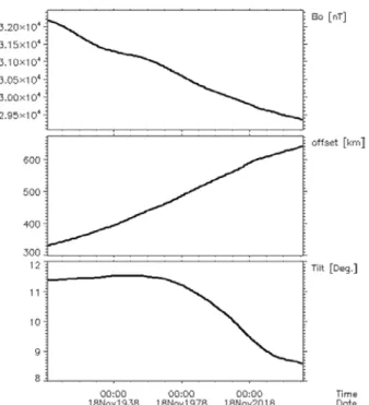
The parameters of a tilted eccentric dipole [8] best fitting IGRF-12 or IPGP-forecast versus time from 1900 to 2050 are shown in Fig. 1. Clearly, those parameters do not evolve linearly with time. From 1900 to 2050, the magnetic field
the dipole with respect to the Earth’s center always increases. Note also that the tilt of the dipole with respect to the Earth’s rotation axis remained almost constant between 1900 and 1950 but has been decreasing since 1950. The Earth’s main magnetic field intensity at 800 km altitude is given in Fig. 2 for years 1900 (top), 1970 (middle) and 2050 (bottom). The shape and location of the South Atlantic Anomaly (SAA) evolve with time. This anomaly drifts to the west and its surface (for a given iso-contour) expands with time. Note that the magnetic field map of year 1970 obtained from IGRF-12 is very close to the Jensen & Cain [9] field model being used in AP8min. In contrast, one can see that in the future (e.g. 2050, as shown in Fig. 2 bottom panel) the topology of the SAA is expected to be significantly different from that seen in 1970.
Fig. 1: Parameters of a tilted eccentric dipole best fitting IGRF-12 (or IPGP-forecast) versus time between 1900 and 2050.
Fig. 2: Magnetic field intensity (nT) at 800 km altitude for year 1900 (top), 1970 (middle) and 2050 (bottom). The red dashed line indicates the magnetic equator.
III. LOW ALTITUDE TRAPPED PROTONS
Because energetic protons are trapped by the Earth magnetic field at low L (the McIlwain parameter [10]) shells, the topology of radiation belts is very much driven by the magnetic field itself. At low altitude, where the magnetic field is dominated by the Earth’s internal field, proton radiation belts will be sensitive to its secular drift. Boscher et al. [1] showed that taking into account the effect of the drift of the SAA over a given time range on the trapped particle distribution at a given L shell (L<2.5) and altitude is equivalent to consider the change in the maximal equatorial pitch-angle (angle between the particle velocity vector and the magnetic field at the magnetic equator) that can be measured at the same L and altitude over the same time range.
To compute the Maximum equatorial Pitch-Angle (MePA) found at a given L, altitude and time, the following approach was implemented:
• A longitude-latitude map of L shells is first computed with a 1° resolution at the given altitude (Fig. 3);
• A primary value of equatorial pitch-angle versus L is deduced (Fig. 4);
• A high resolution map of L shells is next computed with a resolution of 0.1° within ±10° around the first MePA location
• A high precision MePA versus L is finally deduced.
Fig. 3: Longitude-latitude map of the Lshell parameter at 825 km altitude from IGRF-12 in 2010.
Fig. 4: Deduced equatorial pitch-angle at 825 km altitude for various L shells from IGRF-12 in 2010 in the southern hemisphere.
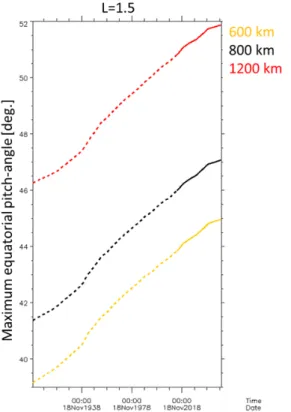
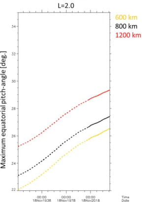
The drift of the MePA at three given altitudes (600, 800 and 1200 km) from year 1900 to year 2050 is shown in Fig. 5 at L=1.5 and in Fig. 6 at L=2. Clearly, on such a long time-range (150 years) this drift is not a linear function of time. Note, however, that from 1978 to 2012 the linear assumption made by Boscher et al. [1] is fully compliant with these new results. The y scale in Fig. 5 and in Fig. 6 being the same, it is clear that at all altitudes the MePA drift becomes more pronounced as L decreases.
Fig. 5: Drift of the MePA computed at L=1.5 for three altitudes from year 1900 to 2050; IGRF-12 is used for the time period 1900-2015 (dashed line) while the IPGP-forecast is used for the time period 2015-2050 (solid line).
Fig. 6: Drift of the MePA computed at L=2. for three altitudes from year 1900 to 2050; IGRF-12 is used for the time period 1900-2015 (dashed line) while the IPGP-forecast is used for the time period 2015-2050 (solid line).
The impact of relying on a truncation at LT=6 for the IPGP
prediction, whereas IGRF-12 was computed up to LT=10, has
also been investigated. To this purpose, the MePA was
re-computed using IGRF-12 with truncation degrees LT equal to
2, 4 and 6, and compared to the reference results obtained with
LT=10. The results for L=1.2 at an altitude of 500 km are
shown in Fig. 7. Clearly, an IGRF-12 field model truncated at
LT=2 is insufficient to compute an accurate value of MePA.
Increasing LT improves the accuracy. At LT=4, results are
already found to be decent for low L (1.2 to 1.5) and good for
higher L values. At LT=6 they are found to be very good for
all L. The mean deviations over 1900-2015 in the 1.1-2 L and
500-1200 km altitude ranges are shown in Fig. 8 for LT=4 and
in Fig. 9 for LT=6. While in the first case a maximum mean
MePA deviation of 1.5% can be found, it drops always below 1% in the second case. Relying on a spherical harmonic
expansion of the Earth’s internal magnetic field up to LT=6
thus appears to be sufficient to describe trapped particles at low altitudes.
Fig. 7: Drift of the MePA computed at L=1.2 and an altitude of 500 km between 1900 and 2015, using IGRF-12 truncated at LT=2, 4, 6 and 10.
Fig. 8: Mean deviations of MePA values computed using IGRF-12 truncated at LT=4 with respect to MePA values computed using IGRF-12 truncated at LT=10 over the 1900-2015 time range.
Fig. 9: Mean deviations of MePA values computed using IGRF-12 truncated at LT=6 with respect to MePA values computed using IGRF-12 truncated at LT=10 over the 1900-2015 time range.
This new long-term assessment of the MePA drift versus L shells (1<L<2.5) and altitudes (400 km<altitude<1400 km) has next been implemented in the OPAL model [1]. It will be released to the public via the GREEN-p model [11] and implemented in the OMERE tool [12].
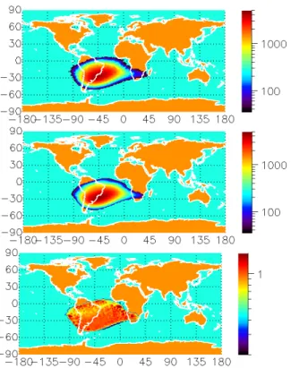
In Fig. 10, we show the predicted longitude-latitude maps of trapped proton flux with E>82 MeV at 800 km altitude for epochs 1900, 1970 and 2050 when using the updated OPAL model. For comparison, we also show 2050 predictions when using AP8min. As expected, between 1900 and 2050 the SAA has drifted to the West and the overall shape of the SAA has changed while the peak flux is almost comparable. Note however, that the shape of the SAA from the perspective of trapped proton flux does not exactly reflect the shape of the SAA as seen in the field intensity (compare Fig. 10 and Fig. 2, in particular for epoch 1900, when the SAA low field intensity overlapped with the dip-equator, leading to a distinct signature in the proton flux SAA). Note also that the forecasted SAA from OPAL in 2050 exhibits significant deviations in location and shape from that provided by AP8min. This is attributed to the lack of magnetic field secular drift compensation in AP8min as it depends on the Jensen & Cain field model from year 1970. Of course those deviations become larger and larger as epoch difference from 1970 increases.
Fig. 10: Trapped proton flux [cm-2s-1] with E>82 MeV at an altitude of 800 km predicted from the updated OPAL model in 1900 (top panel), 1970 (second panel from top) and 2050 (third panel from top) and predicted from AP8min in 2050 (bottom panel). The dashed black line indicates the magnetic equator.
Detailed comparisons between OPAL predictions and in-situ measurements from POES series [13] are shown in Fig. 11 to Fig. 14. Fig. 11 shows the >82 MeV proton fluxes at 800 km altitude in a longitude-latitude map from POES-06 (top panel) and from OPAL (middle panel) in 1979. Note that POES-06 data were projected down to 800 km altitude considering
constant L, B/Beq. One can see the very good match between
in-situ data and the OPAL model prediction. The ratio between >82 MeV proton flux measured by POES-06 and OPAL prediction is given in the bottom panel. In most of the SAA, this ratio is close to 1. Largest deviations (dark red and dark blue) are found at the outer edge of the SAA where proton fluxes are expected to be low. The distribution of these
ratios is plotted in Fig. 12 for fluxes >100 cm2s-1. As can be
seen, 28.7% of points are within 5% error, 55% of points are within 10% error and 81.2% of points are within 20% error. The spread of the distribution around 1 is attributed to statistical uncertainties in the SEM2 instrument count rates (see irregularities in the top panel of Fig. 11). Similar plots using POES-19 for comparison are shown for year 2010 in Fig. 13 and Fig. 14. Again, the OPAL model matches very nicely the in-situ data (for fluxes >100 cm2s-1 it is found that 31% of points are within 5% error, 55% of points are within 10% error and 80.4% of points are within 20% error). Note in particular that the OPAL model properly accounts for the
Fig. 11: >82 MeV protons flux (cm2s-1) provided by POES-06 at 800 km altitude in 1979 (top panel), and predicted by OPAL (middle panel); also shown the ratio between OPAL predictions and POES-06 measurements (bottom panel).
Fig. 12: Distribution of the ratio of OPAL predictions to POES-06 measurements for the >82 MeV flux in 1979.
Fig. 13: >82 MeV protons flux (cm2s-1) provided by POES-19 at 800 km altitude in 2010 (top panel), and predicted by OPAL (middle panel); also shown the ratio between OPAL predictions and POES-19 measurements (bottom panel).
Fig. 14: Distribution of the ratio of OPAL predictions to the POES-19 measurements for >82 MeV flux in 2010.
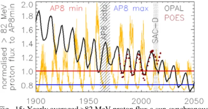
To illustrate the impact of the OPAL predictions on spacecraft specifications, the yearly averaged >82 MeV proton flux a sun-synchronous spacecraft would encounter at an altitude of 800 km has been computed between 1900 and 2050 (Fig. 15). The yearly averaged >82 MeV proton flux obtained from the NOAA-POES series (06, 08, 10, 12, 15 and 19) at the same altitude is also reported on this plot. Note that flux values are normalized to AP8min. As mentioned in [1], low altitude proton fluxes are modulated by the solar cycle, i.e. F10.7 radio flux, with a time lag depending on the energy, the amplitude of the peak flux being anti-correlated to the F10.7 radio flux. For predictions beyond 2015, a conservative approach was used and a very weak solar cycle (via the F10.7 radio flux) was considered (see orange curve in Fig. 15). The >82 MeV proton fluxes from the OPAL model normalized to AP8min at 800 km altitude exhibit a global trend over more than a century: the trapped proton flux decreases due to the secular drift of the magnetic field (see Fig. 1). This decrease is not linear with time and strongly depends on the offset and tilt of the eccentric dipole best describing the Earth’s core magnetic field. Fig. 15 leads us to conclude that:
- AP8min generally underestimates proton fluxes at
energies > 82 MeV and at 800 km altitude. This is true even during the time period when proton data being used to produce AP8 model were measured
(see the hatched polygon in Fig. 15, deduced from [14]): a maximum factor between 1.3-1.4 is found right after the 1964 solar minimum.
- the >82 MeV proton fluxes found between 2011 and
2015 are compliant with conclusions from [10], where it was found that AP8min was underestimating both the TNID measured by ICARE-NG onboard SAC-D by 10.7% [15], and the cumulated SEU number from EDAC implemented onboard the CRYOSAT-2 altimeter by 16% [15].
- OPAL slightly underestimates >82 MeV proton
fluxes at 800 km after 2013 (by about 10%). Note that OPAL was developed in 2013 and that recent POES data during the current weak solar cycle were therefore not yet available. So far this 10% discrepancy is attributed to the F10.7 dependence of the model rather than to the Earth’s core magnetic field. It is suspected that our assumption of a dependence on F10.7 with an energy dependent lag time is not yet sufficient: to further refine the model, the time derivative of F10.7 should also be considered (while during the extended solar minimum period from 2007 to 2009, the F10.7 index remained almost constant and very low, the >82 MeV proton flux was still increasing. Because OPAL only depends on F10.7 and not on its time derivative, this feature cannot be captured by the model).
- The amplitude of the energetic proton flux
modulation is linked to the solar cycle amplitude. The global decrease of energetic proton flux (on the very long term, i.e. several solar cycles) is linked to the secular drift of the Earth’s core magnetic field.
- The >82 MeV proton flux is expected to be lower
than predicted by AP8min in future years.
Fig. 15: Yearly averaged >82 MeV proton flux a sun-synchronous spacecraft at an altitude of 800 km would encounter. Results are normalized to AP8min predictions. Dots refer to proton flux obtained from the NOAA-POES series (06, 08, 10, 12, 15 and 19) normalized to APmin predictions. The red line indicates the reference, i.e. AP8min, and the blue line refers to AP8max normalized to AP8min predictions.
IV. CONCLUSIONS
The secular drift of the Earth’s main field has been implemented in the OPAL model and is now available from years 1900 to 2050. A slow decrease of energetic low altitude proton fluxes along time is predicted, reflecting the secular drift of the Earth’s core magnetic field. The solar cycle
modulation introduced in the OPAL model reproduces POES flight data with high fidelity during the active solar cycles 21, 22 and 23. During the weak solar cycle 24, OPAL predictions are underestimating POES data by about 10%. This discrepancy will be investigated in the near future and is attributed to the F10.7 dependency during weak solar cycles. Keeping in mind this limitation, it is found that:
- AP8min underestimates energetic trapped proton
fluxes by about 30% in the 1970s and by 20% in the 1980s to 2000s years on average over a full solar cycle.
- This deviation is expected to be smaller in a near
future and to reverse after 2025, when AP8min would then overestimate energetic trapped proton fluxes.
REFERENCES
[1] Boscher, D., Sicard-Piet, A., Lazaro, D., Cayton, T., & Rolland, G., A new proton model for low altitude high energy specification. IEEE Transactions on Nuclear Science, 61(6), 3401-3407, 2014.
[2] D.M. Sawyer, J.I. Vette, “AP-8 trapped proton environment for solar maximum and solar minimum”, NSSDC/WDC-A-R&S, 76-06, NASA/GSFC, Greenbelt, MD (1976).
[3] E. Thébault, C. Finlay, C Beggan, P. Alken, J. Aubert, O. Barrois, F. Bertrand, T. Bondar, A. Boness, L. Brocco, E. Canet, A. Chambodut, A. Chulliat, P. Coïsson, F. Civet, A. Du, A. Fournier, I. Fratter, N. Gillet, B. Hamilton, M. Hamoudi, G. Hulot, T. Jager, M. Korte, W. Kuang, X. Lalanne, B. Langlais, J.M. Léger, V. Lesur, F. Lowes, S. Macmillan, M. Mandea, C. Manoj, S. Maus, N. Olsen, V. Petrov, V. Ridley, M. Rother, T. Sabaka, D. Saturnino, R. Schachtschneider, O. Sirol, A. Tangborn, A. Thomson, L. Tøffner-Clausen, P. Vigneron, I. Wardinski, and T. Zvereva, “International Geomagnetic Reference Field: the 12th generation”, Earth, Planets and Space, 67:79, 2015.
[4] Aubert, .J., C.C. Finlay, and A. Fournier, Bottom-up control of geomagnetic secular variation by the Earth’s inner core, Nature, 502, 219-223
[5] Aubert, J., “Flow throughout the Earth's core inverted from geomagnetic observations and numerical dynamo models”, Geophysical Journal International, 192(2), 537-556, 2013.
[6] Fournier, A., J. Aubert, and E. Thébault, “A candidate secular variation model for IGRF-12 based on swarm data and inverse geodynamo modelling”, Earth, Planets and Space 67:81, 2015.
[7] Aubert, J., “Geomagnetic forecasts driven by thermal wind dynamics in the Earth's core”, Geophysical Journal International 203, 1738-1751, 2015.
[8] Fraser-Smith, A.C., Centered and Eccentric Geomagnetic Dipoles and their poles, 1600-1985, Reviews of Geophysics, 25(1), 1-16, 1987. [9] Jensen D.C. and J.C. J. Cain, “An interim geomagnetic field”, Geophys.
Res., 67, pp. 3568-3569, 1962Sicard, A., Boscher, D., Bourdarie, S., Lazaro, D., Standarovski, D., and Ecoffet, R., “GREEN: the new Global Radiation Earth ENvironment model (beta version)”, In Annales Geophysicae (Vol. 36, No. 4, pp. 953-967). Copernicus GmbH, 2018. [10] McIlwain, C. E., Coordinates for mapping the distribution of
magnetically trapped particles. Journal of Geophysical Research, 66(11), 3681-3691, 1961.
[11] Sicard, A., Boscher, D., Bourdarie, S., Lazaro, D., Standarovski, D., & Ecoffet, R.. GREEN: the new Global Radiation Earth ENvironment model (beta version). In Annales Geophysicae (Vol. 36, No. 4, pp. 953-967). Copernicus GmbH, 2018.
[12] http://www.trad.fr/en/space/omere-software/ , 2018. [13] ftp://satdat.ngdc.noaa.gov , 2018
[14] S.F. Fung, “Recent development in the NASA trapped radiation models”, Radiation Belts: Models and Standards, Ed. J. Lemaire et al., Geophysical Monograph 97, AGU, Washington (USA), 79, 1997. [15] Bourdarie S. et al., "Benchmarking Ionizing Space Environment
Models," in IEEE Transactions on Nuclear Science, vol. 64, no. 8, pp. 2023-2030, Aug. 2017.
![Fig. 10: Trapped proton flux [cm -2 s -1 ] with E>82 MeV at an altitude of 800 km predicted from the updated OPAL model in 1900 (top panel), 1970 (second panel from top) and 2050 (third panel from top) and predicted from AP8min in 2050 (bottom panel](https://thumb-eu.123doks.com/thumbv2/123doknet/14799993.605729/6.918.475.856.80.562/trapped-proton-altitude-predicted-updated-opal-second-predicted.webp)