Uncertainties associated with digital elevation models for hydrologic applications: a review

(1)

HAL Id: hal-00298756

https://hal.archives-ouvertes.fr/hal-00298756

Submitted on 28 Aug 2006

HAL is a multi-disciplinary open access

archive for the deposit and dissemination of sci-entific research documents, whether they are pub-lished or not. The documents may come from teaching and research institutions in France or abroad, or from public or private research centers.

L’archive ouverte pluridisciplinaire HAL, est destinée au dépôt et à la diffusion de documents scientifiques de niveau recherche, publiés ou non, émanant des établissements d’enseignement et de recherche français ou étrangers, des laboratoires publics ou privés.

Uncertainties associated with digital elevation models

for hydrologic applications: a review

S. Wechsler

To cite this version:

S. Wechsler. Uncertainties associated with digital elevation models for hydrologic applications: a review. Hydrology and Earth System Sciences Discussions, European Geosciences Union, 2006, 3 (4), pp.2343-2384. �hal-00298756�

(2)

HESSD

3, 2343–2384, 2006 Uncertainties associated with digital elevation models S. Wechsler Title Page Abstract Introduction Conclusions References Tables Figures J I J I Back Close

Full Screen / Esc

Printer-friendly Version

Interactive Discussion

Hydrol. Earth Syst. Sci. Discuss., 3, 2343–2384, 2006 www.hydrol-earth-syst-sci-discuss.net/3/2343/2006/ © Author(s) 2006. This work is licensed

under a Creative Commons License.

Hydrology and Earth System Sciences Discussions

Papers published in Hydrology and Earth System Sciences Discussions are under open-access review for the journal Hydrology and Earth System Sciences

Uncertainties associated with digital

elevation models for hydrologic

applications: a review

S. Wechsler

California State University Long Beach, 1250 Bellflower Boulevard, Long Beach CA 90840, USA

Received: 24 April 2006 – Accepted: 23 June 2006 – Published: 28 August 2006 Correspondence to: S. Wechsler (wechsler@csulb.edu)

(3)

HESSD

Full Screen / Esc

Abstract

Digital elevation models (DEMs) represent the topography that drives surface flow and are arguably one of the more important data sources for deriving variables used by numerous hydrologic models. A considerable amount of research has been conducted to address uncertainty associated with error in digital elevation models (DEMs) and the 5

propagation of error to derived terrain parameters. This review brings together a dis-cussion of research in fundamental topical areas related to DEM uncertainty that affect the use of DEMs for hydrologic applications. These areas include: (a) DEM error; (b) topographic parameters frequently derived from DEMs and the associated algorithms used to derive these parameters; (c) the influence of DEM scale as imposed by grid cell 10

resolution; (d) DEM interpolation; and (e) terrain surface modification used to generate hydrologically-viable DEM surfaces. Each of these topical areas contributes to DEM uncertainty and may potentially influence results of distributed parameter hydrologic models that rely on DEMs for the derivation of input parameters. The current state of research on methods developed to quantify DEM uncertainty is reviewed. Based on 15

this review, implications of DEM uncertainty and suggestions for the GIS research and user communities emerge.

1 Introduction

The general purpose of this review is to examine the nature, relevance and manage-ment of digital elevation model (DEM) uncertainty in relation to hydrological applica-20

tions. DEMs provide a model of the continuous representation of the earth’s elevation surface. This form of spatial data provides a model of reality that contains deviations from the truth, or errors. The nature and extent of these errors are often unknown and not readily available to users of spatial data. Nevertheless, DEMs are one of the most important spatial data sources for digital hydrologic analyses as they describe the 25

(4)

HESSD

Full Screen / Esc

however uncertainty in the DEM representation of terrain through elevation and derived topographic parameters is rarely accounted for by DEM users (Wechsler, 2003). DEM uncertainty is therefore of great importance to the hydrologic community.

This paper reports on representative literature on DEM uncertainty as applied to hydrologic analyses1. To understand how to address and manage DEM uncertainty, 5

specifically in relation to hydrologic applications, it is necessary to recognize the com-ponents and characteristics of DEMs that contribute to that uncertainty. This paper provides a review of research in each of these fundamental areas which includes: (a) DEM error; (b) topographic parameters frequently derived from DEMs and the asso-ciated algorithms used to derive these parameters; (c) the influence of DEM scale as 10

imposed by grid cell resolution; (d) DEM interpolation; and (e) terrain surface modifica-tion used to generate hydrologically-viable DEM surfaces. Each of these topical areas contribute to DEM uncertainty and potentially influence results of distributed parameter hydrologic models that rely on DEMs for the derivation of input parameters. The cur-rent state of research on methods developed to quantify DEM uncertainty is reviewed. 15

Based on this review, implications of DEM uncertainty and suggestions for the research and GIS user communities emerge.

In the past decade DEM data has become increasingly available to spatial data users due to the decrease in data and computer costs and the increase in computing power. DEMs produced from technologies such as Light Detection and Ranging (LiDAR) and 20

IFSAR (Interferometric Synthetic Aperture Radar sensor) are more readily available. These remotely-sensed DEM production methods provide users with high resolution DEM data that have stated vertical and horizontal accuracies in centimeters, making them more desirable, yet costly in both dollars and processing requirements. DEM users with limited budgets can obtain DEMs from government sources or conduct field 25

surveys using global positioning systems (GPS) and interpolate DEMs for smaller study

1

Given the burgeoning nature of this literature, it regrettably has not been possible to cite every publication on this topic. An attempt has been made to give examples of studies related to focal variables.

(5)

HESSD

Full Screen / Esc

areas. No matter the source, DEM products provide clear and detailed renditions of topography and terrain surfaces. These depictions can lure users into a false sense of security regarding the accuracy and precision of the data. Potential errors, and their effect on derived data and applications based on that data, are often far from users’ consideration (Wechsler, 2003).

5

In colloquial terms, error has a negative connotation indicating a mistake that could have been avoided if enough caution had been taken (Taylor, 1997). However, errors are a fact of spatial data and are not necessarily bad as long as they are understood and accounted for. There has been much discussion in the literature regarding philoso-phies (Fisher, 2000), ontologies (Worboys, 2001), and definitions (Heuvelink, 1998; 10

Refsgaard et al., 2004) of spatial data uncertainty. For the purposes of this discussion of DEM uncertainty, the term error refers to the departure of a measurement from its true value. Uncertainty is a measure of what we do not know about this error and its impact on subsequent processing of the data. In the spatial realm, errors and resulting uncertainty can never be eliminated.

15

Our responsibilities as DEM data users and researchers are to accept, search for and recognize error, strive to understand its nature, minimize errors to the best of our technical capabilities, and obtain a reliable estimate of their nature and extent. Based on these understandings, the tasks are to develop and implement methods to quantify and communicate the uncertainty associated with the propagation of errors in 20

spatial data analyses. The research reported in this paper brings together knowledge about the components and characteristics of DEM uncertainty specifically related to hydrologic applications

2 DEM error

Errors in DEMs generate uncertainty. DEM errors are related to various DEM sources, 25

structures and production methods, and are generally categorized as either systematic, blunders or random (USGS, 1997). Systematic errors result from the procedures used

(6)

HESSD

Full Screen / Esc

in the DEM generation process and follow fixed patterns that can cause bias or artifacts in the final DEM product. When the cause is known, systematic bias can be eliminated or reduced. Blunders are vertical errors associated with the data collection process and are generally identified and removed prior to release of the data. Random errors remain in the data after known blunders and systematic errors are removed.

5

Sources of DEM errors have been described by Burrough (1986); Wise (1998) and Heuvelink (1998). Numerous studies have evaluated error and accuracy of various DEM products. These include DEMs produced from synthetic aperture radar (SAR) (Wang and Trinder, 1999), the Shuttle Radar Topography Mission (SRTM) (Suna et al., 2003; Miliaresis and Paraschou, 2005), USGS DEMs (Berry et al., 2000; Shan et al., 10

2003), and comparisons of various DEM production methods (Li, 1994). Methods to assess and reduce DEM error have been developed (Li, 1991; Lopez, 2002; Hengl et al., 2004). DEM errors have been related to production methods and terrain complexity; increased errors have been correlated with terrain complexity.

DEM accuracy is usually quantified using the RMSE statistic. While a valuable quality 15

control statistic, the RMSE does not provide an accurate assessment of how well each cell in a DEM represents a true elevation. Furthermore, the RMSE is based on the assumption of a normal distribution (Monckton, 1994), which is often violated in the case of the DEM. DEM quality can be assessed by conducting ground truth surveys that can be time intensive and costly.

20

It has been suggested that assessment of DEM uncertainty requires more informa-tion on the spatial structure of DEM error – beyond that provided by the RMSE. DEM vendors have been urged to provide additional DEM quality information such as “maps

of local probabilities for over or underestimation of the unknown reference elevation val-ues from those reported in the DEM, and joint probability valval-ues attached to different

25

spatial features.” (Kyriakidis et al., 1999, p. 677). The reality is that information beyond

the RMSE will not be provided to DEM users nor will most users take the time or spend the money to obtain such data sets in order to conduct DEM error assessment (Wech-sler, 2003). Because information on sources of error are not readily available, it is often

(7)

HESSD

Full Screen / Esc

difficult, if not impossible, to recreate the spatial structure of error for a particular DEM. Knowledge about the spatial structure of error is an important component for gaining an understanding of where errors arise and uncertainty is propagated. Methods should accommodate detailed DEM error information when available, yet provide mechanisms for addressing uncertainty in the absence of this information.

5

3 Computation of topographic parameters for hydrologic analyses

The DEM provides a base data set from which topographic attributes are digitally generated. The raster grid structure lends itself well to neighborhood calculations which are frequently used to derive these parameters. Primary surface derivatives such as slope, aspect and curvature provide the basis for characterization of landform 10

(Evans, 1998; Wilson and Gallant, 2000). These terrain attributes are used exten-sively in hydrologically-based environmental applications and are derived directly from the DEM. The routing of water over a surface is closely tied to surface form. Flow di-rection is derived from slope and aspect. From flow didi-rection, the upslope area that contributes flow to a cell can be calculated, and from these maps, drainage networks, 15

ridges and watershed boundaries can be identified. Topographic, stream power, radi-ation, and temperature indices are all secondary attributes computed from DEM data. Wilson and Gallant (2000) provide a detailed review of the DEM-derived primary and secondary topographic attributes. Research has demonstrated that DEM-derived to-pographic parameters are sensitive to both the quality of the DEMs from which they 20

are generated (Bolstad and Stowe, 1994; Wise, 2000) and the algorithms that are used to produce them. This section discusses the calculation of certain topographic parameters from DEMs.

Numerous algorithms exist for calculating topographic parameters. For example, slope is calculated for the center cell of a 3×3 matrix from values in the surrounding 25

eight cells. Algorithms differ in the way the surrounding values are selected to com-pute change in elevation (Skidmore, 1989; Carter, 1990; Guth, 1995; Dunn and Hickey,

(8)

HESSD

Full Screen / Esc

1998; Hickey, 2001). Different algorithms produce different results for the same derived parameter and their suitability in representing slope in varied terrain types may differ. The slope algorithm developed by Horn (1981) and currently implemented in ESRI GIS products is thought to be better suited for rough surfaces (Horn, 1981; Burrough and McDonnell, 1998). The slope algorithm presented by Zevenbergen and Thorne (1987), 5

currently implemented in the IDRISI GIS package (Eastman, 1992), is thought to per-form better in representing slope on smoother surfaces (Zevenbergen and Thorne, 1987; Burrough and McDonnell, 1998).

The routing of flow over a surface is an integral component to the derivation of subse-quent topographic parameters such as watershed boundaries, and channel networks. 10

Many different algorithms have been developed to compute flow direction from gridded DEM data and are referred to as single or multiple flow path algorithms. The single flow path method computes flow direction based on the direction of steepest descent in one of the 8 directions from a center cell of a 3×3 window (Jenson and Domingue, 1988), a method referred to as D8. The D8 algorithm is the flow direction algorithm that 15

is provided within mainstream GIS software packages (such as ESRI GIS). However, the users in the hydrologic community recognize that the D8 approach oversimplifies the flow process and is insufficient in its characterization of flow from grid cells. In re-sponse, researchers have developed multiple flow path methods that distribute flow in all possible down-slope directions, rather than just one; see for example (Quinn et al., 20

1991; Costa-Cabral and Burgess, 1994; Wolock and McCabe, 1995; Tarboton, 1997; Zhou and Liu, 2002). Multiple flow path methods attempt to approximate flow on the sub-grid scale. Multiple flow path functions are currently not part of standard GIS pack-ages and are therefore not readily available to DEM users. Desmet and Govers (1996) compared six flow routing algorithms and determined that single and multiple flow path 25

algorithms produce significantly different results. Thus any analysis of contributing ar-eas such as watersheds or stream networks will be greatly affected by the algorithm implemented. Other approaches to deriving channel networks and watershed bound-aries have been developed such as those that incorporate additional environmental

(9)

HESSD

Full Screen / Esc

characteristics (Vogt et al., 2003).

Unfortunately, GIS packages do not differentiate between rough and smooth surfaces when applying a slope or provide users with ay options when it comes to derivation of terrain parameters. Users cannot choose a particular method; only one algorithm for derivation of parameters such as slope, aspect and flow direction is embedded in a par-5

ticular GIS software package. This lack of flexibility in software capability introduces the likelihood of further error transferred to derived topographic parameters. Additional re-search on the appropriateness of certain algorithms for various terrain types is needed. Future GIS software packages should accommodate research needs by providing flex-ibility in the algorithms available to users. Software vendors will hopefully integrate the 10

research produced by the hydrologic community in order to yield “smarter” GISs that are capable of evaluating a DEM, and then apply an appropriate algorithm to specific areas based on terrain characteristics and complexity.

4 DEM resolution and scale for representing topography

Theobald (1989) noted that “. . . seldom are errors described in terms of their spatial 15

domain, or how the resolution of the model interacts with the relief variability” (p. 99).

This continues to be a concern.

The raster GIS grid cell data structure makes it possible to represent locations as highly defined discrete areas. The grid cell size imposes a scale on raster GIS analy-ses. It is also a representation of the spatial support which in geostatistics refers to the 20

area over which variables are measured (Heuvelink, 1998; Dungan, 2002). The size of a grid cell is commonly referred to as the grid cell’s resolution, with a smaller grid cell indicating a higher resolution. DEM accuracy has been shown to decrease with coarser resolutions that average elevation within the support (Li, 1992). Smaller grid cell sizes allow better representation of complex topography and these high resolution 25

DEMs are better able to refine characteristics of complex topography. This has led many DEM users to seek the highest DEM resolutions possible, increasing the costs

(10)

HESSD

Full Screen / Esc

associated with both data acquisition and processing. However, is higher resolution necessarily better? To what extent is the grid cell resolution a factor in the propagation of errors from DEMs to derived terrain parameters?

The literature has established that the grid cell size of a raster DEM significantly af-fects derived terrain attributes (Kienzle, 2004). The impact of grid cell resolution on ter-5

rain parameters has been related to both topographic complexity and the nature of the algorithms used to compute terrain attributes. A variety of algorithms have been used to compute slope from grid-DEMs using various grid cell resolutions. In each case, as the DEM resolution became finer the calculated maximum slope became larger (Carter, 1990; Chang and Tsai, 1991; Jenson, 1991; Bolstad and Stowe, 1994; Gao, 1997; Yin 10

and Wang, 1999; Toutin, 2002; Armstrong and Martz, 2003). This effect is related to the topography’s complexity. If topography is complex, greater discrepancies can be expected between grid cells.

Grid resolution has been shown to impact the accuracy of hydrologic derivatives in the following applications: topographic index (Quinn et al., 1991; Quinn et al., 1995; 15

Valeo and Moin, 2000), drainage properties such as channel networks and flow ex-tracted from DEMs (Garbrecht and Martz, 1994; Wang and Yin, 1998; Tang et al., 2001; Lacroix et al., 2002), the spatial prediction of soil attributes (Thompson et al., 2001), computation of geomorphic measures such as area-slope relationships, cu-mulative area distribution and Strahler stream orders (Hancock, 2005), flow, direction 20

calculations (Usul and Pasaogullari, 2004), modeling processing of erosion and sedi-mentation (Schoorl et al., 2000), computation of soil water content (Kuo et al., 1999) and output from the popular rainfall-runoff model TOPMODEL (Saulnier et al., 1997; Brasington and Richards, 1998).

DEM resolution has also been shown to directly impact hydrologic model predictions 25

from TOPMODEL (Wolock and Price, 1994; Zhang and Montgomery, 1994; Band and Moore, 1995; Quinn et al., 1995), the SWAT model (Chaplot, 2005; Chaubey et al., 2005), and the Agricultural Nonpoint Source Pollution (AGNPS) (Vieux and Needham, 1993; Perlitsh, 1994). The Water Erosion Prediction Project (WEPP) model, however,

(11)

HESSD

Full Screen / Esc

was not sensitive to coarser resolution DEMs unless the resolution compromised wa-tershed delineation (Chochrane and Flanagan, 2005).

Research has demonstrated that higher resolution is not necessarily better when it comes to the computation of DEM derived topographic parameters (Wechsler, 2000; Zhou and Liu, 2004). Higher resolution DEMs generate larger slope values. This can 5

be attributed to the nature of the slope algorithm in which the grid cell resolution is e ffec-tively the “run” in the rise-over-run formula. Smaller grid cells therefore compute larger slope values. Research to determine an appropriate grid cell resolution for particular analyses has also been undertaken (Albani et al., 2004; Kienzle, 2004). However, se-lection of an appropriate resolution will depend on characteristics of the study area and 10

nature of the analysis.

The repeated outcomes of the effects of grid cell resolution in various hydrologic ap-plications suggest that grid cell resolution will remain an important factor in our under-standing, assessment and quantification of the propagation of DEM errors to hydrologic parameters and resulting uncertainty in related modeling applications.

15

Variability at scales larger than those captured by the grid cell area, referred to as sub-grid variability, exists, but has for the most part, been ignored. To date, sub-grid information is either unavailable or lost through interpolation techniques. However, as technologies progress and more and more data becomes available from DEM produc-tion methods (such as LiDAR which produces millions of data points used for DEM 20

interpolation), sub-grid information could be retained. Methods to differentiate data from noise will need to be developed. This additional information could become a useful component for future DEM uncertainty estimations.

5 Interpolation

Some researchers generate surfaces for areas not covered by existing data or in situ-25

ations where the surface must be of greater accuracy or more detailed resolution than existing data. Based on a survey of DEM users, seventeen percent indicated that they

(12)

HESSD

Full Screen / Esc

generate their own DEM surfaces data (Wechsler, 2003). The proliferation of LiDAR data requires users to interpolate DEMs from millions of delivered points. A detailed review of various interpolation approaches can be found in (Burrough, 1986; Wood, 1996; Burrough and McDonnell, 1998). Often little is known about the error either oc-curring during or generated as a result of the interpolation process (Desmet, 1997). 5

The accuracy of surfaces generated by interpolation is difficult to assess, unless a sur-face of known higher accuracy is available for comparison. This latter situation is rare because the presence of a high accuracy surface precludes the need for interpolation. A validation procedure can be applied in the absence of higher accuracy data whereby interpolation points are removed and saved as a validation data set for comparison 10

with the interpolated surface. Usually, a “good” surface is one that is found to most closely match the input data, as quantified using the RMSE computed from validation data obtained from the same data source (Maune, 2001). The relative accuracy of self-generated surfaces is linked to both the interpolation method and the grid cell size selected for interpolation. It is necessary to recognize the combined influence of these 15

factors on the accuracy of the resulting surface.

Uncertainty associated with interpolation procedures has been a focus of practition-ers and researchpractition-ers in the geostatistical community (Dubois et al., 1998). Off-the-shelf GIS packages allow users to perform interpolation using a variety of interpolation meth-ods, most notably inverse distance weighing, spline and Kriging. Other methods have 20

been developed (Bindlish and Barros, 1996; Doytsher and Hall, 1997; Shi and Tian, 2006). However, relatively few studies explicitly address the impact that different inter-polation methods have on a resulting DEM. Wood and Fisher (1993) and Wood (1996) applied visualization techniques to identify DEM interpolation errors. Desmet (1997) investigated the effect of interpolation on precision (accuracy of the predicted heights) 25

and shape reliability (degree of fidelity in the spatial pattern of topography) expressed by derived topographic parameters. Wise (1998) investigated the effect of interpolating DEMs from contours using different algorithms. Differences in results were attributed to the complex interactions between algorithms for both interpolation and derivation of

(13)

HESSD

Full Screen / Esc

DEM-derived topographic parameters (Wise, 1998). Erxleben et al. (2002) evaluated the accuracy of snow water equivalents derived from DEMs generated using four inter-polation methods. Kienzle (2004) tested the quality of DEMs interpolated at different resolutions and identified an optimum grid cell size that was determined to be between 5–20 m depending on terrain complexity.

5

Additional research would assist in increasing our understanding of the impact that DEM interpolation methods have on propagation of error to derived parameters and uncertainty. Validation and cross validation techniques can provide a mechanism for quantifying accuracy and developing models for the spatial structure of DEM error, which in turn can be used to quantify uncertainty as it propagates to derived parameters 10

and the models that use them.

6 Surface modification for hydrologic analyses

Overland flow routing through grid cells of a DEM requires a DEM without disruptions. DEMs often contain depressions that result in areas described as having no drainage, referred to as sinks or pits. These depressions disrupt the drainage surface, which 15

preclude routing of flow over the surface. Sinks arise when neighboring cells of higher elevation surround a cell, or when two cells flow into each other resulting in a flow loop, or the inability for flow to exit a cell and be routed through the grid (Burrough and McDonnell, 1998; ESRI, 1998). Hydrologic parameters derived from DEMs, such as flow accumulation, flow direction and upslope contributing area, require that sinks be 20

removed. This has become an accepted and common practice.

To use a DEM as a data source in hydrologic analyses, sinks must be removed, a “necessary evil” according to Burrough and McDonnell (1998) and Rieger (1998). Sinks, however, can be real components of the surface. For example in large scale data where surface hummocks and hollows are of importance to surface drainage flow, 25

sinks are accurate features. With the advent of high resolution (submeter grid cell) DEMs it is possible that sink filling operations will be costly not only in processing time,

(14)

HESSD

Full Screen / Esc

but in removing naturally occurring features of the terrain surface.

Naturally occurring sinks in elevation data with a grid cell size of 100 m2or larger are rare, although they could occur in glaciated or karst topography (Mark, 1988; Tarboton et al., 1993). To date, sinks have been treated as artifacts of the DEM creation method and eliminated by various techniques. However, with the proliferation of high resolution 5

(<0.25 m2) DEMs, sinks that represent naturally occurring features of the topography, such as hummocks and hollows, that are found in glaciated terrain, should not be treated as artifacts.

A number of methods have been described for eliminating depressions in DEMs (O’Callaghan and Mark, 1984; Jenson and Domingue, 1988; Hutchinson, 1989; Jen-10

son, 1991; Rieger, 1998; Martz and Garbrecht, 1999). Off-the-shelf GIS packages such as the ESRI suite of software use a sink filling approach based on the D8 single flow direction flow routing method first described by Jenson and Domingue (1988) and Jenson (1991). This sink filling approach raises the sink elevation to that which enables flow linkage. This approach has the disadvantage of assuming that all depressions are 15

due to an underestimation of elevation in the sink, rather than the overestimation of surrounding cells, and flow routing is based on the D8 single-direction flow algorithm discussed previously. Other algorithms have been developed that incorporate the mul-tiple flow path approach that more adequately addresses the nature of depressions (Rieger, 1998; Martz and Garbrecht, 1999).

20

While research has focused on the development of sink filling methods, little attention has been paid to either the appropriateness of a particular sink filling algorithm or to the impact of the sink filling operation on DEMs and derived parameters. Wechsler (2000) investigated the impact of DEM errors and the sink filling procedure on representation of elevation and derived parameters using a Monte Carlo simulation technique. The 25

effect of sink filling was quantified directly for elevation and slope and indirectly for the TI. While there was no significant difference between elevation from filled and unfilled DEMs, a significant bias was observed in the slope parameter. The sink filling pro-cedure raised the elevation of cells where sinks were found, increasing elevations in

(15)

HESSD

Full Screen / Esc

these areas, resulting in a larger positive bias for elevation. Raising these elevations in turn decreased slope estimators in these areas, leading to negative bias for slope. Sink filling did not appear to have a significant impact on the calculation of the topographic index. These findings have implications for watershed studies conducted in lower lying, flatter areas such as agricultural watersheds

5

Lindsay and Creed (2005) investigated the occurrence of depressions in remotely sensed DEMs representing varying terrain types (flat to mountainous). As would be expected, the number of depressions found was related to grid cell resolution, and flat areas experienced more depressions than high-relief landscapes. They found that flat areas, valley bottoms and highly convergent topography were most likely to experience 10

depressions.

In addition to the process of sink filling, hydrologists frequently undertake another a method of surface modification referred to as stream burning, to generate “hydrologi-cally enforced” DEMs (Maune, 2001). The method integrates vector representation of hydrography with the interpolation of the DEM. This automatic adjustment of the DEM 15

has been incorporated into the ANUDEM package (Hengl et al., 2004; Hutchinson, 2006). The impact of this surface modification procedure on derived parameters has not been addressed in the literature.

7 Distributed Parameter Hydrologic Models

“GIS do not “create” information. However there appears to have developed an implicit

20

reliance on GIS to provide information adequate to parameterize physically based dis-tributed hydrological models, often at spatial resolution and accuracy levels that are unrealistic given the original source of spatial data.” (Band and Moore, 1995, p. 419).

GISs are designed to represent environmental features, such as topography, which drive dynamic hydrologic (and other environmental) processes. Although they are not 25

designed to serve as dynamic modeling tools (Reitsma and Albrecht, 2005) the ability of the GIS to represent the distributed nature of data sets lends itself well as a platform

(16)

HESSD

Full Screen / Esc

for integrating distributed hydrologic models.

Topography is the driving force behind the hydrologic response of a watershed. Hydrologic processes are represented by and analyzed using hydrologic models. Many hydrologic models are distributed in nature; terrain representation is divided into smaller areas or grid cells within which hydrologic processes are simulated. The raster 5

grid structure allows flow to be routed through the watershed via grid cells. This struc-ture integrates well with distributed parameter hydrologic models that are designed to accept grid-based inputs such as derived topographic parameters. Grid-based DEMs have been used ubiquitously to generate input parameters such as slope gradient, as-pect, curvature, flow direction and upslope contributing area, for distributed parameter 10

hydrologic models (Johnson and Miller, 1997; Saghafian et al., 2000; Armstrong and Martz, 2003).

The use of a GIS to generate input parameters for distributed parameter models en-ables a watershed to be analyzed at higher resolutions than would be practical using manual methods. The distributing of hydrologic information imposes an inherent scale 15

on hydrologic analyses that must be recognized. The effect of this scale is often not acknowledged and the results of the effects of this scale are neither quantified nor con-sidered when presenting results from various hydrologic models. Sensitivity analyses are frequently performed by hydrologists on model inputs such as hydrograph estima-tions, and Manning’s roughness coefficients. However, they are rarely performed on 20

DEM-derived attributes such as slope, aspect and flow direction. This leads to a num-ber of questions such as: What is the appropriate grid cell resolution for a hydrologic analysis? How does uncertainty propagate from the DEM to input parameters and through the models?

As discussed above, outputs from distributed parameter hydrologic models such as 25

WEPP, SWAT, AGNPS and TopModel have been shown to be highly sensitive to grid cell size. Lagacherie et al. (1996) evaluated the propagation of error in topographic parameters through a hydrologic model to simulate flood events. Variations in outputs were documented and were not linear. Differences in DEM vertical accuracies were

(17)

HESSD

Full Screen / Esc

shown to impact the accuracy of runoff predictions from the soil-hydrology-vegetation model (DHSVM) (Kenward et al., 2000).

Hydrologic models are complex. Identifying sources of error in DEMs is difficult enough. Understanding their propagation to topographic parameters compounds the problem. Understanding how the errors in these parameters in turn affect physically 5

based models continues to be a challenge. Practitioners often undertake hydrologic analyses with a hope that error propagation to hydrologic parameters is minimal when combined within hydrologic models. However, is it safe to make this assumption without assessing or reporting the uncertainties associated with input parameters, especially those derived from DEMs? Research has indicated that even small discrepancies can 10

have a meaningful impact on the results of hydrologic models, and could influence the way hydrologic information, as represented by hydrologic models is evaluated and interpreted. Users of hydrologic models must be aware of the influence that both the DEM and GIS software have on the calculation of various model parameters. The task ahead is to develop accepted methodologies for quantifying and communicating 15

propagation of these errors to results of hydrologic analyses.

8 DEM uncertainty simulation

“Even with an understanding of the size and texture of spatial data uncertainty, it is not possible to determine what is actually “out there” as long as there is any amount of uncertainty. All that can be achieved is the generation of representations of what may

20

potentially be there, and the use of these potential realizations to develop a stochastic understanding of how spatial data uncertainty affects a geographic information appli-cation of any complexity” (Ehlschlaeger, 1998, p. 6).

The previous sections identified issues associated with DEM error and the use of DEMs in hydrologic analyses. The next section describes approaches to address DEM 25

uncertainty.

(18)

HESSD

Full Screen / Esc

(1) reporting descriptive statistics or accuracy statistics such as the Root Mean Square Error (RMSE), (2) creation of error maps (3) visualization techniques and (4) application of simulation techniques to model DEM error propagation. While the RMSE accuracy statistic provides a general indication of DEM quality, it is a summary statistic and does not provide information on the spatial structure, nature and extent of DEM errors. 5

DEM error cannot be characterized by just one number (Heuvelink, 2002). An error map approach that requires a source of higher accuracy data can add information by indicating the spatial structure of DEM errors. However, it may be unreasonable to expect that DEM users will have access to higher accuracy data from which an error map can be computed. Visualization techniques may be valuable in conveying the 10

implications of potential inaccuracies inherent in DEM data sets, however they are often not accompanied by quantitative results. On their own, these first three approaches are not sufficient approaches to the characterization of DEM uncertainty. However, when used in conjunction with simulation techniques the combination presents a powerful means to portray results of uncertainty analyses.

15

8.1 Stochastic simulation

A stochastic representation of uncertainty provides a distribution of potential answers, from which a “good” answer can be chosen, given some predefined criteria. The stochastic approach to DEM error modeling requires a number of equally probable realizations upon which selected statistics are performed. Uncertainty is quantified by 20

evaluating the statistics associated with the range of outputs. Stochastic simulations provide a series of random equiprobable maps. Simulation does not ensure that a “real” map is generated from the process, but provides a distribution of results within which we can state the “true” map lies (Chrisman, 1989; Journel, 1996). Much re-search has focused on the use of stochastic simulation techniques to propagate error 25

and quantify uncertainty in spatial data (Heuvelink et al., 1989; Openshaw et al., 1991; Goodchild et al., 1992; Brunsdon and Openshaw, 1993; Veregin, 1994). While various simulation techniques are available (Deutsch and Journel, 1998), Monte Carlo

(19)

simu-HESSD

Full Screen / Esc

lation has been most commonly applied to assess DEM uncertainty, possibly due to its simplicity in approach and general applicability. This technique assumes that the DEM is only one realization of a host of potential realizations. Surfaces are randomly perturbed to create new DEM realizations that yield a probability distribution of pos-sible outcomes. An alternative to Monte Carlo simulation is an approach that applies 5

an analytical model of error propagation based on a Taylor Series expansion (see for example Albani et al., 2004; Bachmann and Allgower, 2002; Heuvelink, 1998; and Heuvelink et al., 1989). For the purposes of this review, methods based on the Monte Carlo simulation approach are discussed.

8.2 DEM error simulation: case atudies 10

“...there is no inherent reason why conditional simulation should not be used as rou-tinely for uncertainty analysis as kriging is used for interpolation. It is unlikely, however, that conditional simulation will become available in the GIS environment until a substan-tial demand has been established...this is likely to require the gradual accumulation of case studies in the literature...” (Englund, 1993 p. 437).

15

The high frequency of studies that use Monte Carlo simulations to assess uncertainty indicates that this is a preferred method for quantifying DEM uncertainty and its propa-gation to DEM-derived surfaces. Resulting case studies differ in approaches applied to generate random error fields, and particular DEM derivatives assessed. Approaches to random field generation reflect two different philosophies about the nature of DEM 20

error: heuristic versus empirical. The empirical approaches assume that the spatial structure of DEM error is available and can be integrated into random field generation. This requires access to a higher accuracy data source from which this information can be derived. The heuristic approaches assume that no prior knowledge of DEM error is available; higher accuracy data can be difficult and costly to obtain. In the absence of 25

this information, random fields can be approximated by the accuracy statistic (RMSE) provided with DEM metadata. As the following case studies demonstrate, progress has been made in demonstrating the applicability and effectiveness of these varied

(20)

ap-HESSD

Full Screen / Esc

proaches to error propagation within a Monte Carlo Simulation. However the two error propagation approaches indicate that an agreed approach to a “best practice” is as of yet unresolved.

8.2.1 Heuristic random fields

The heuristic approach to error propagation is based on the RMSE provided with a 5

DEM data set. In this approach, any value in the DEM has the possibility of being the stated elevation, or any value within a normally distributed range of the RMSE. Random error fields with a mean of zero and a standard deviation equivalent to the RMSE are generated and added to the original DEM to create a DEM realization. Multiple realiza-tions of the DEM provide a Gaussian distribution that better represents the DEM under 10

uncertain conditions (Hunter and Goodchild, 1997; Fisher, 1998). However, Tobler’s First Law of Geography – everything is related to everything else, but near things are more related than distant things – cannot be ignored (Tobler, 1970). Elevation is spa-tially autocorrelated, and therefore, it is understood that elevation errors are spaspa-tially autocorrelated.

15

In one of the earliest studies, Goodchild (1980) outlined a procedure for generating errors with specified spatial autocorrelation as measured by the Moran’s “I” statistic. Later studies built on this approach. Lee et al. (1992) found that floodplain delin-eations were significantly affected by DEM error. Fisher (1993) simulated the impact of DEM error on viewshed analyses using this method and determined that DEM-derived 20

viewsheds may overestimate the ”true” viewshed. Davis and Keller (1997) modified the Goodchild (1980) approach to model uncertainty in slope stability prediction. The modified method was used to increase spatial autocorrelation in error field generated by variogram analyses. The authors suggested that this method could be improved by incorporating autocorrelation at different levels of aggregation based on slope classes, 25

user defined windows or slopes. Hunter and Goodchild (1997) applied a spatially au-toregressive random field method that incorporates spatial autocorrelation of DEM er-ror. This method was compared with completely random, uncorrelated error fields to

(21)

HESSD

Full Screen / Esc

assess the effect of these error representations on slope and aspect calculations. The authors concluded that an error model ought to be based on an assumption of spa-tial dependence of error; however, completely random fields could be applied in the absence of a higher accuracy surface from which to obtain this information. The Good-child (1980) method was also adapted by Veregin (1997) to incorporate slope in the 5

iterative swapping approach. In this approach, slope served as an underlying indicator of the spatial distribution of DEM error. Flow paths derived from DEMS using the D8 method were found to be sensitive to DEM errors, especially in areas of low slope.

Murillo and Hunter (1997) applied the spatially autocorrelation iterative swapping method to evaluate the effect of DEM error on prediction of areas susceptible to land-10

slides. While uncertainty associated with some model input such as choice of slope classes and slope algorithms were acknowledged it was not addressed. Uncertainty results were communicated through visualization via map output. Wechsler (2000) and (Wechsler and Kroll, 2006) compared simulations resulting from four different methods of random fields that included completely random (mean of 0 and standard deviation 15

equal to the RMSE) and three different filter methods that increased the spatial autocor-relation of the error fields. Wechsler (2000) applied this method to evaluate the effects of DEM uncertainty on sink filling, topographic parameters calculated at different reso-lution, and topographic parameters computed for different terrain types. Although less sophisticated than the iterative swapping method to achieving spatial autocorrelation, 20

the methodology was implemented directly via an extension to a commonly used GIS software package. Widayati et al. (2004) implemented the error propagation methods presented by Wechsler (2000) to evaluate the propagation of elevation error on flat and varied slopes and differing grid resolutions. Slope error was found to be sensitive to the spatial dependence of DEM error. Cowell and Zeng (2003) assessed uncertainty 25

in the prediction of coastal hazards due to climate change. Uncertainty in the DEM was represented by random, normally distributed error fields. As error was increased, model output uncertainty decreased due to the nature of the normal distribution of the error fields used. Yilmaz et al. (2004) evaluated uncertainty in flood inundation which

(22)

HESSD

Full Screen / Esc

was represented probabilistically based on results of a Monte Carlo simulation using completely random fields with a normal distribution based on the RMSE.

More recently, a “process convolution” or spatial moving averages approach to the generation of random error fields was used to evaluate the delineation of drainage basins that were found to be very sensitive to DEM uncertainty (Oksanen and Sar-5

jakoski, 2005a). The approach was applied to both slope and aspect derivatives and demonstrated that completely random uncorrelated random error fields may be a valid mechanism for representing DEM error (Oksanen and Sarjakoski, 2005b).

Methods for assessing DEM uncertainty through simulation and error propagation have not been fully integrated into assessing hydrologic model output with the excep-10

tion of Zerger (2002) who investigated the effect of DEM uncertainty on a storm surge model. The DEM was interpolated using ANNUDEM, and random error fields were spatially autocorrelated. DEM errors impacted low inundation scenarios. This spatial uncertainty was communicated using visualization through risk maps.

8.2.2 Empirical random fields 15

Another school of thought on error propagation assumes that the RMSE alone is an insufficient indicator of DEM error, and that additional knowledge of the spatial struc-ture of error in a particular DEM is required for uncertainty modeling in a Monte Carlo simulation. Approaches have been developed that incorporate higher accuracy data, such as that garnered from a higher accuracy DEM or GPS survey, to develop a model 20

of the spatial structure of error, which in turn is used to generate DEM realizations. Ehlschlaeger and Shortridge (1996) developed a model that creates random fields with a Gaussian distribution that matches the mean and standard deviation derived from a higher accuracy data source. Spatial autocorrelative characteristics of spa-tially dependent uncertainty are accounted for in the algorithm that was applied to a 25

least-cost-path application. Kiriakidis et al. (1999) present a geostatistical approach to DEM realizations that incorporate autocorrelation information derived from residuals obtained from higher accuracy sources. Holmes et al. (2000) applied this approach to

(23)

HESSD

Full Screen / Esc

the prediction of slope failure. Endreny and Wood (2001) evaluated the effect of DEM error on flow dispersal area predictions using six different algorithms. Error fields were spatially autocorrelated based on an error matrix derived from an assessment of dif-ferences between the test USGS 30 m DEM and a higher resolution 10m SPOT DEM. Uncertainty results were communicated using probability maps. Ehlschlaeger (2002) 5

introduced a method for generating error fields that accounts for both the spatial au-tocorrelation of error and incorporates information about DEM characteristics such as topological shapes in the error model. Canters et al. (2002) evaluated the effects of DEM error on a landscape classification model. Random error fields were spatially correlated using error characteristics derived from a ground truth survey. While uncer-10

tainty caused by image classification was found to be more significant than DEM error, transition zones were particularly sensitive to DEM error. Van Niel et al. (2004) applied Monte Carlo simulation to assess the impact of DEM uncertainty on slope, aspect, net solar radiation, topographic position and topographic index. The error in these DEM-derived parameters was propagated to results of a vegetation model. DEM error was 15

assessed by comparison with a higher accuracy data source obtained from a GPS survey and used to filter normally distributed random error fields.

Each of these case studies demonstrates the applicability of the Monte Carlo simu-lation approach to error propagation and uncertainty assessment in DEMs and DEM-derived data. The remaining challenge is to provide these approaches as tools that 20

DEM users can readily access through GIS software packages. There will be occa-sions when a DEM user has access to a higher accuracy data source for generating information on the spatial structure of error, and there will be occasions when that infor-mation is unavailable. The ultimate DEM uncertainty toolbox should provide simulation approaches that accommodate both these scenarios as part of its error propagation 25

(24)

HESSD

Full Screen / Esc

9 Integrating and communicating DEM uncertainty

“. . . The absence of facilities within GIS software for handling the effects of input data uncertainty and possible error propagation by GIS operations creates a question mark over the safe utilization of many aspects of the technology. . . ” (Openshaw et al., 1991, p. 78).

5

Methods have been developed that transfer information from a GIS into external er-ror propagation analysis tools (see for example Heuvelink, 1998; Hwang et al., 1998). Output from these external systems is either returned to the GIS for mapping and vi-sualization or exported to graphic charts or statistical tables. Attempts have also been made to integrate uncertainty simulation tools within a GIS (Wechsler, 2000; Wechsler 10

and Kroll, 2006). However, a viable DEM uncertainty toolbox that incorporates various simulation approaches, and considers the fundamental areas that contribute to DEM uncertainty described herein has not yet been realized. What are the essential compo-nents of a viable DEM uncertainty toolbox and what form should it take? How should simulation results be quantified and communicated?

15

9.1 User interfaces: Decision Support Systems

Assessment of the multiple fundamental factors that contribute to DEM uncertainty and their propagation to topographic parameters and hydrologic models is complex. The ability of a user to interact with and explore possible outcomes is crucial for informed decision making. Spatial decision support systems (SDSS) provide a mechanism for 20

integrating data exploration and assessing model outcome to facilitate informed deci-sion making and can serve as a mechanism for achieving this interaction with DEM users. An SDSS is generally comprised of a spatial database and a user-defined inter-face that accesses GIS analysis and modeling capabilities. Multiple Criteria Decision Models (MCDM) are a type of SDSS that allow users to make decisions with multiple 25

alternatives (Jankowski et al., 2001; Ascough et al., 2002).

(25)

un-HESSD

Full Screen / Esc

certainty assessment. However, many GIS user interfaces can now be modified and enhanced through object-oriented programming that allows users to develop tools to assess model results and assist in decision making based on these results. Such direct integration of decision support tools that incorporate uncertainty theory within a GIS has been achieved on a limited basis. Wechsler (2000) and (Wechsler and 5

Kroll, 2006) integrated a toolbox within a GIS to allow users to simulate the effects of DEM error on elevation, slope, upslope area and the topographic index. While results were not carried through to a particular hydrologic modeling effort, and used simple error propagation techniques, the approach demonstrated how these tools can be in-tegrated as pull-down-menus into mainstream GIS. Aerts et al. (2003) developed an 10

SDSS external to a GIS to assess the impact of DEM uncertainty on a cost-path analy-sis for ski run development. Although uncertainty associated with specific model input parameters such as slope cannot be culled out, and the product is not specifically part of a GIS package, the research successfully demonstrates the efficacy of such an approach. Gunther (2003) developed a software program called SLOPEMAP, that in-15

tegrates with two commonly used terrain analysis packages (ArcView GIS and Surfer) to derive geologic information from a DEM for assessment of rockslide susceptibility. Debruin and deWit (2005) developed a method to streamline the evaluation of grids within a stochastic simulation. This computer application demonstrates progress in the use of Monte Carlo simulations on desktop computers. Currently some GIS packages 20

have limitations on the number of grids that can be assessed simultaneously. Other ef-forts to develop GIS-based decision support tool are notable. Wise et al. (2001) report on the results of the successful integration of a GIS-based user interface for statistical spatial data analysis. Dura ˜nona and Lopez (2000) developed a toolbar to detect errors in a DEM. Crosetto and Tarantola (2001) present general procedures for assessment of 25

uncertainty within a GIS-based flood forecasting model. Each of these studies demon-strates the viability of the SDSS as a mechanism for addressing DEM uncertainty, and integrating that knowledge with specific distributed parameter hydrologic models. The manner in which results of these simulations can be communicated is varied.

(26)

HESSD

Full Screen / Esc

9.2 Visualization

“A number of visualization tools need to be developed to portray error at the same time as the original data. The increasing use of computer displays and the development of stochastic models of error present the opportunity for doing just this.” (Fisher, 1994 p. 181).

5

Results of methods to assess DEM uncertainty must be effectively communicated in order to be integrated and applied. Cartographic representations are the primary method of communicating results from GIS-based spatial analyses, and the main com-municative output provided by GISs. DEM uncertainty can be visualized in a number of ways including static tables or graphs, error maps of residuals between a DEM and a 10

higher accuracy data source, error matrices, static maps or map animations of realiza-tions from Monte Carlo Simularealiza-tions (Wood, 1996; Davis and Keller, 1997; Ehlschlaeger et al., 1997; Ehlschlaeger, 1998). Other efforts have integrated tools within the GIS in-terface. This section discusses progress in these areas.

Visualization techniques have been applied to evaluate and convey the potential 15

inaccuracies inherent in DEM data sets such as DEM error (Acevedo, 1991), interpo-lation accuracy (Wood and Fisher, 1993; Wood, 1996) and results of DEM uncertainty simulations (Hunter and Goodchild, 1995). Spear et al. (1996) conducted a survey to investigate the effectiveness of different visualization techniques in conveying DEM interpolation uncertainty. Map animations have been used to visualize uncertainty in 20

image classification (Zhang and Stuart, 2001) and a slope stability model Davis and Keller (1997). Jankowski et al. (2001) investigated the role of maps as visual tools in the data exploration and decision making process. A user interface was developed that allows users to interactively visualize the results of certain input assumptions. While a DEM was not part of this particular analysis, the approach could be followed to develop 25

methods to assess DEM uncertainty.

Visualization of uncertainty alone may not be an efficient method for communicating uncertainty to the decision maker. Quantitative estimates of error and their

(27)

conse-HESSD

Full Screen / Esc

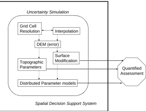
quences, if available, should be either incorporated into the visualization or reported. What should a hydrologically-based DEM uncertainty SDSS toolbox look like and how should results be communicated? Research and technology demonstrate that the in-tegration of simulation research with hydrologic models is possible. Cartographic re-search continues to focus on communication approaches. Distributed hydrologic mod-5

els vary extensively and therefore uncertainty results will vary based on the distributed model applied. A modular DEM error assessment system would be capable of break-ing up the component uncertainties and assessbreak-ing the impact of error on model outputs (see for example Fig. 1). For such a system to be successful, continued research is required to assess the human component, to determine to what extent and in what 10

format users are willing to accept, address and manage error.

10 Conclusions

How users and decision makers react to and work with error and uncertainty and results based on uncertain data continues to present a challenge (Heuvelink and Burrough, 2002). The following pronouncement aptly summarizes the state of this domain of 15

research and applications:

“. . . Although considerable progress has been made in the theory and practice of data quality and error propagation in numerical modeling with GIS, there is still a long way to go before we have a coherent and comprehensive toolkit for general applica-tion. The ideal future. . . in which both data quality assessment and error propagation

20

are essential ingredients for an intelligent GIS, has not yet been reached. . . .it is also essential to convince our colleagues in the user community that these new methods and procedures are being developed to help them make better decisions and not just to make life difficult. The sociology of how people deal with the problems of spatial data quality also needs to be addressed, and just as with the development of improved

25

methods, this forms an important challenge for the coming years. . . ” (Heuvelink and Burrough, 2002, p. 113).

(28)

HESSD

Full Screen / Esc

While not exhaustive, this comprehensive review attempts to identify the fundamental issues associated with DEMs as applied to hydrologic applications. This review brings together a discussion of research in topical areas related to DEM uncertainty that affect the use of DEMs for hydrologic applications.

Research has established that DEMs contain errors that propagate to derived topo-5

graphic parameters. Such errors are influenced by DEM resolution and interpolation methods. DEMs used for hydrologic applications are frequently further modified by either filling depressions or burning streams. These areas: DEM error, topographic parameter generation, grid cell resolution, interpolation and hydrologic modifications are all essential considerations when undertaking an assessment and quantification 10

of DEM uncertainty, and should be considered in the development of an uncertainty toolbox integrated within an spatial decision support system (SDSS).

DEM uncertainty simulation methodologies have been developed and some assess-ments of the effect of DEM uncertainty on specific hydrologic models have been eval-uated in case studies. Although progress has been made, these approaches are far 15

from being implemented as a spatial decision support system for DEM users. The paradigm of an “uncertainty button” (Goodchild et al., 1999) or uncertainty toolbox pro-vided by vendors and implemented by users is not yet a reality. Yet is such an invention even a viable option? Sentiment has been expressed that due to the complexity of the topic, an uncertainty toolbox is a fantasy. Uncertainty assessment is thought to require 20

too much processing time and considerable prior knowledge is required of the DEM users (Heuvelink, 2002). DEM users are not likely to be willing to spend time on uncer-tainty assessment (Wechsler, 2003) unless it becomes a simplified and cost-effective exercise that can be justified in “billable hours”.

The call for a DEM uncertainty toolbox echoes that of previous researchers and the 25

GIS community. This has not yet been satisfactorily achieved in the decade-or-so since it was first suggested, probably due to a combination of technology limitations, software limitations and DEM user limitations. However, as a discipline, the hydrologic GIS user community is ready to progress in this area. Technology limitations are continuing to

(29)

HESSD

Full Screen / Esc

be overcome; computer processing power has increased and Monte Carlo simulations on raster grids can now be performed on most desktop computers.

Yes, DEM uncertainty assessment and management is complex and challenging, yet it is a mandatory undertaking to the progression of hydrologic science. In hydro-logic modeling, sensitivity analyses are frequently performed on certain non-spatial 5

model parameters as part of model calibration activities. Guidelines for assessing data uncertainty in essential components of river basin studies have been proposed (van Loon and Refsgaard, 2005), yet sensitivity analyses are not routinely performed on hydrologic model parameters derived from DEMs. The uncertainties associated with DEM-derived model inputs must be addressed in order to have confidence in model 10

predictions, and for decisions based on modeling output to hold up in court, should they go that far. DEM errors and resulting uncertainty may not have an influence on specific hydrologic model results, but is it appropriate to make this assumption without testing it?

This paper presents a challenge to the entire GIS community which includes ven-15

dors, researchers, educators, and users: communicate, educate, develop and imple-ment. Awareness of uncertainty must be raised within the broader GIS community. The perception of uncertainty and error as “bad” must be altered. The expressed futility due to the complexity of the issues can be overcome.

Educators must instill the concept of GIS as a fact of spatial data that must and can 20

be acknowledged and addressed. This could begin with a bottom-up effort initiated by GIS software developers. They could provide users with choices in both algorithms and approaches to deriving parameters frequently used in hydrologic analyses, specif-ically slope and flow direction. This simple modification would raise user awareness regarding the existence of these different algorithms, and could be an important first 25

step toward an intelligent GIS that can accommodate uncertainty. Once these options are integrated into mainstream GIS, users will become more receptive to the concept of multiple plausible answers to an analysis rather than one grid as the “correct” deriva-tive from a DEM. Future software developments might include a GIS that can sense

(30)

HESSD

Full Screen / Esc

differentiation in terrain complexity. Specific grid cell resolutions and terrain attribute algorithms could then be applied to areas of the DEM as appropriate rather than taking a “one size fits all” approach. Methods to determine an appropriate grid cell resolution for interpolating a terrain surface can be integrated and computed in the background, so that users can either choose a resolution or use one that has been “suggested” by 5

behind-the scene computations and data exploration in the intelligent GIS. Ultimately, the DEM uncertainty toolbox would provide a mechanism for users to simulate the ef-fect of DEM error (whether higher accuracy data is available, or not) derive a series of plausible outcomes for particular distributed parameter hydrologic models, and com-municate model results visually and quantitatively given DEM uncertainty. Perhaps 10

once these buttons become part of the DEM processing “toolbox”, users may become more receptive to using an SDSS that allows users to simulate DEM uncertainty and incorporate uncertainty output into analytical results that inform decision makers with greater accuracy.

DEM error exists and results of analyses that rely on DEM data will always have a 15

component of uncertainty. Uncertainties in DEMs and DEM related applications are bound to increase as GIS becomes an increasingly mature science; this is a sign of progress rather than limitation in technology (Dungan, 2002) but must be managed effectively by the GIS community. The field of geographic information systems is pro-gressing toward geographic information science. The technology is applied to invoke 20

the scientific method – hypothesize, experiment, ask spatial questions and explore observations. As the GI-Science movement progresses from the academic/research communities to the practitioner/user communities, developers will be expected to inte-grate research, such as that reviewed here, into DEM uncertainty assessment tools. Research has demonstrated ways to account for and communicate DEM uncertainty 25

through simulation modeling and visualization. Software vendors could incorporate these modeling and visualization methods into products through SDSS interfaces. SDSS interfaces should be designed in response to research on: How do users in-teract with uncertain data? What type of interface will users be most receptive to; what