Two-dimensional simulations of a curved shock: Self-consistent formation of the electron foreshock

HAL Id: hal-01646986

https://hal.archives-ouvertes.fr/hal-01646986

Submitted on 4 Aug 2020

HAL is a multi-disciplinary open access

archive for the deposit and dissemination of

sci-entific research documents, whether they are

pub-lished or not. The documents may come from

teaching and research institutions in France or

abroad, or from public or private research centers.

L’archive ouverte pluridisciplinaire HAL, est

destinée au dépôt et à la diffusion de documents

scientifiques de niveau recherche, publiés ou non,

émanant des établissements d’enseignement et de

recherche français ou étrangers, des laboratoires

publics ou privés.

Two-dimensional simulations of a curved shock:

Self-consistent formation of the electron foreshock

Philippe Savoini, Bertrand Lembège

To cite this version:

Philippe Savoini, Bertrand Lembège. Two-dimensional simulations of a curved shock: Self-consistent

formation of the electron foreshock. Journal of Geophysical Research Space Physics, American

Geo-physical Union/Wiley, 2001, 106 (A7), pp.12975 - 12992. �10.1029/2001JA900007�. �hal-01646986�

JOURNAL OF GEOPHYSICAL RESEARCH, VOL. 106, NO. A7, PAGES 12,975-12,992, JULY 1, 2001

Two-dimensional

simulations

of a curved

shock'

Self-consistent

formation

of the electron

foreshock

Philippe S•voini •nd Bertrand Lemb•ge

Centre d'6tude des Environnements Terrestre et Plan6taires, CNRS, Universit6 de Versailles-St Quentin, V61izy, France

Abstract. A collisionless curved shock is analyzed in a supercritical regime with the help of a two-dimensional electromagnetic full particle code. Curvature effects are included self-consistently and allow one to follow continuously the transition from a narrow and step-like strictly perpendicular shock to a wider and more turbulent oblique shock within the quasi-perpendicular range 65 ø < OB,, < 90 ø. Present

results reproduce the formation of the electron foreshock without any simplifying

shows

that local back-streaming

distributions

have two components:

(i) a high

by a field-aligned

bump-in-tail or beam signature,

and (ii) a low-energy

parallel

component

characterized

by a loss

cone

signature

(mirrored

electron). Two types of

pattern evidenced

experimentally

(narrow type). These also confirm

that mirroring

1. Introduction

The foreshock is the region of space extending be- tween the curved shock layer and the upstream mag- netic field lines tangent to the shock; this region is char- acterized by the presence of energetic particles back- streaming upstream away from the shock front along magnetic field lines connected to the curved shock. Since the early seventies, this region has been exten-

sively studied both theoritically [Leroy and Mangehey,

1984; Wu, 1984; Cairns, 1987; Krauss-Vatban and Wu,

1989; Fitzenreiter et al., 1990] and experimentally IFil-

bert and Kellogg, 1979; Anderson et al., 1979; Ander- son, 1981; Parks et al., 1981; Feldman et al., 1973, 1982,

1983; Klimas, 1985], and more recently, this region has

been studied with the WIND spacecraft, which provides in situ measurements of high sensitivity and resolution

[Fitzenreiter et al., 1996; Lepping et al., 1995; Slavin et al., 1996; Yin et al., 1998a], and the GEOTAIL mission [Kasaba et al., 1997].

Copyright 2001 by the American Geophysical Union.

Paper number 2001JA900007.

0148-0227/01/2001JA900007 $09.00

The general consensus is that the foreshock electron

population is composed of incoming solar wind electrons

and a small number of bow shock modified electrons

that stream back into the upstream region. These back-

streaming electrons have two components, which can

be described in terms of time of flight and generalized mirroring processes as follows:

1. One component corresponds to electrons which, after interacting with the shock front, succeed to es- cape from the front and stream back along upstream magnetic field lines. Moreover, these electrons are con- vected back with magnetic field lines because of the

earthward motion of the solar wind (E x B drift caused by the solar wind's motional electric field) and are spa-

tially diffuse acc.ording to their parallel velocities. Then the velocity distribution at a given upstream observa- tion point is the sum of contributions determined by ve- locity characteristics connecting different source points

on the curved shock to the observer location. The ef-

fect analyzed by Filbert and Kellog [1979] and further developed by Cairns [1987] is called the time-of-flight

mechanism.

2. The other component corresponds to electrons which are mirror reflected by the shock front. Indeed,

12,976 SAVOINI AND LEMBlb, GE: 2-D SIMULATION OF ELECTRON FORESHOCK

the shock front can be seen as a moving magnetic mir- ror structure, depending on which reference frame the process is viewed. It is convenient to discuss the mir-

ror reflection process in the deHoffman-Teller (dHT)

frame defined by a motional transformation along the shock surface in which the flow of the upstream plasma is parallel to the magnetic field and the induced mo-

tional electric field vanishes. Electron acceleration has

been analyzed theoretically in dHT by Leroy and Man-

geney [1984] and Wu [1984], who assumed an elastic

encounter between electrons and a moving plane shock

front. Krauss-Varban and Wu [1989] have shown that

efficiency of this acceleration mechanism is similar in

both dHT and normal incident (NI) frames. This en-

ergization mechanism is also called fast Fermi process

[Wu, 1984] or gradient-B drift process [Krauss-Varban and Wu, 1989], since the reflection mechanism can be

very efficient and does not require multiple interactions with the shock. The theory has shown satisfactory agreement with observational data and emphasizes the importance of the nearly perpendicular shocks as natu- ral energizers of the solar wind electrons population.

In summary, theory predicts that electron energiza- tion by mirror effects is weakly sensitive to the shock structure but is quite sensitive to the shock wave ge-

ometry (through a 1/cos0B• term), at least when the

shock is nearly perpendicular; OB• is the angle between the shock normal and the upstream magnetostatic field.

Two main consequences can be deduced [Leroy and Mangehey, 1984; Wu, 1984]:

1. The average

kinetic

parallel

energy

per

reflected

< Erll >m2

meVupstream

2

/ COS

20Bn

(1)

2. In the case of an incoming Maxwellian distribu- tion function, the density of reflected electrons decreases

as exp[-1/cos2(O•3•],

when 0•3,approaches

90

ø. As

a consequence, the number of reflected electrons tends toward 0 at the leading edge of the foreshock, i.e., the magnetic field line tangent to the curved shock front. These calculations have been refined later by Krauss- Vatban and Wu [1989], who expressed the gain of ki-

netic energy versus both the initial energy and pitch angle.

Even if a good qualitative agreement with observa- tion is obtained, it is pertinent to resume the assump- tions used in the analytical works which are not always justified:

1. The theory has been established for angles 0•3, large enough to simplify the calculations and is only

valid around 900 . Nevertheless, the acceleration mech- anism is very sensitive to the angle 0•3, even a small deviation of 0 induces strong variation of the energy

gain (through

the term COS-20Bn

of equation

(1)).

2. Calculations ignore the effect of finite excursion time of electrons in the shock wave during reflection;

in particular, no loss of energy due to waves-electrons interaction is considered during the reflection process.

3. The electron magnetic moment •u is assumed

to be conserved in the reflection process (adiabatic the- ory). First, such an assumption is valid only when the

gyroradius of a convected electron is much smaller than the width of the shock transition layer, which can be inaccurate for high inflow velocities. Second, the as- sumption does not account for magnetic and electric fluctuations seen by the particles during their time of flight in the vicinity of the shock front.

4. Shock front is assumed to be stationary. As al-

ready evidenced by planar one-dimensional (i-D) Leroy et al. [1982] for hybrid simulations and Lemb•ge and Dawson [1987] for full-particle simulations and by two-

dimensional

(2-D) simulations

[Lemb•ge

and Savoini,

1992], the shock front is nonstationary. Two sources of nonstationarity have to be considered [Lemb•ge and Savoini, 1992]: First, the shock front suffers a self-

reformation over a typical timescale of the order of the

ion gyroperiod < •ci >ramp (calculated from the mean value of the magnetic field in the ramp); second, the

front itself exhibits a rippled pattern which moves in time along the shock front direction. Until now, the impact of this shock front nonstationarity on electron acceleration processes has not been analyzed and is still

unknown.

More recently, analytical models of cylindrical and spherical shocks with zero and nonzero thickness have been investigated by Vandas [1995a, 1995b]. These

studies examine the energy gain of reflected individ- ual electrons in the presence of a curved shock in or- der to generalize theoretical results obtained in previ- ous works. The model is based on strong assumptions. First, it solves electron motion in the shock layer with the adiabatic approximation, and it approximates the curved shock near the tangent point of the upstream

magnetic field by a plane shock with varying B• (the

normal component of the magnetic field at the shock

front). Second, it does not take into account the elec- trostatic field (Etx) and the noncoplanar magnetic field

in the shock layer, which are known to play an impor- tant role in the electron dynamic. In this model, the energy gain of reflected electrons is strongly affected by the curvature and, more particularly, is lower than that at a corresponding plane shock. Shock curvature de- creases the time spent by the particle within the shock

layer and so does its total energy gain. A compari-

son with experimental data leads to comparable levels of fluxes for interplanetary shocks but shows sore, dis- crepancies for the Earth's bow shock.

Numerical studies have already investigated the mag-

netic mirror reflection process with test particles and

shock

profiles

issued

from hybrid simulations

[Krauss-

ional hybrid code with macroparticle ions and an in-

SAVOINI AND LEMB]•GE: 2-D SIMULATION OF ELECTRON FORESHOCK 12,977

the shock is well established, energetic electrons which

are assumed

to participate

in the reflection

process

are

injected as test particles and are followed during sev- eral ion gyroperiods. Such simulations are not self- consistent, since this requires the use of full particle codes. In addition, these do not take into account the global curvature of a shock (which requires a 2-D ge- ometry), and these only allow one to investigate the

vicinity of 900 through a model where spatial curva- ture of the electromagnetic components is introduced

via cosine functions. Both Maxwellian and n functions

are used to describe the incident electron population. A reasonable agreement is obtained with experimental data in producing the observed large fluxes of reflected electrons at the Earth's bow shock. Nevertheless, the intrinsic limitations of such hybrid simulations are obvi- ous. The bow shock has a two-dimensional curved pat- tern, and electron foreshock cannot be reproduced with oblique planar shock simulations. In addition, reflected electrons back-streaming along the interplanetary mag- netic field will experience a time-dependent angle 0B,• which can modify the effectiveness of the acceleration

process.

The purpose of the present paper is to present results obtained from full-particle simulations of a 2-D curved shock, where self-consistent features are fully involved and allow one to reproduce the electron foreshock with- out restrictive or ad-hoc assumptions.

The organization of the paper is as follows. Condi- tions of numerical simulations and the method for gen- erating the curved shock are described in section 2. Sec- tion 3 presents the main numerical results; local elec- tron distribution functions are analyzed in detail and are compared to experimental data in section 4. Fi- nally, discussion and concluding remarks are given in

section 5.

2. Numerical Description

Present simulations have been performed with a 2-1/2 dimensional, fully electromagnetic, relativistic particle code using standard finite-size particle techniques. De-

tails have been already given by Lernb•ge and Savoini

[1992]

and $avoini and Lemb&ge

[1994]. Basic

proper-

and plasma. Fields are separated into two sets: The electromagnetic transverse components, hereinafter de- noted by a subscript "t", reflect the induced effects and

are solutions of the full set of Maxwells' equations, and

the electrostatic longitudinal components, hereinafter

denoted by a subscript "l", result from the space-charge effects and are solutions of Poisson's equation. Nonperi- odic conditions are applied along the x direction within

the simulation box and, periodic conditions are used

along

the y direction. Leng•ths

of the plasma

simula-

tion box are L• - 768 and Ly - 1024, which represent

40 and 53 ion inertial lengths

(Y/Spi), respectively.

All

quantities with tildes are in normalized units.

The curved shock is created by using a cylindrical

magnetic piston localized in the vacuum part of the

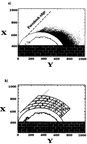
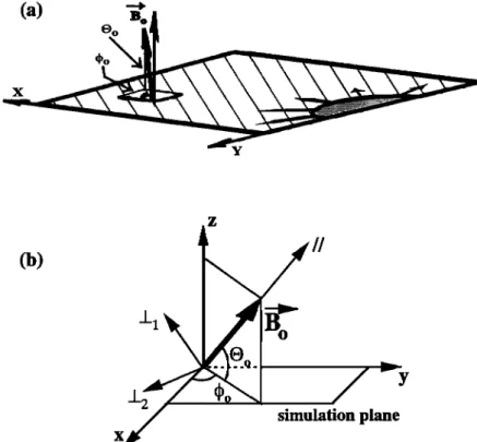
simulation box. This procedure turns out to be very ef- ficient and rapid in terms of computer time. The curved shock propagates through the X- Y simulation plane as illustrated in Figure la.

One important

poi•nt

concerns

the orientation

of the

the simulation plane. We define two angles as shown in Figure lb' q•o and 0o provide the relative orienta- tion of the magnetic field lines within and outside the

X- Y plane,

respectivel•y.

More precisely,

•o is defined

netostatic field Bo and the projection of this field within the simulation plane.

The curvature of the shock front imposes a continuous

variation in the orientation of the local shock normal (always lying within the simulation plane, as illustrated by small arrows in Figure la); this implies an angle

between the upstream magnetic field Bo and ff defined by the relation:

0•,• - arccos

[cos

0o (cos

•o cos

• + sin •o sin •)], (2)

where • is the angle between ff and the X axis. The present study is made for 0o - 650 and •o - 45 ø. The finite value of 0o means that the curved shock is ana- lyzed within a restricted quasi-perpendicular range, i.e., with 0•,• varying from 900 to 650 where the electron ac- celeration is efiqcient, as • varies from •o - 900 to •o.

Such a configuration provides the accessibility for the electrons to flow along the magnetic field lines outside the simulation plane and to have a moderate projected displacement within the X- Y plane. Preliminary sim-

ulations have shown that the case 0•,• - 0 ø (i.e., with Bo fully lying within the simulation plane, 0o - 0 ø)

cannot be reproduced at present time with a reason- able CPU cost, since electrons flow immediately along the field lines before the curved shock is really formed. The radius of the magnetic cylinder has been cho- sen carefully so that, after a short transient period t <_ 0.2Yci, the curvature radius Rc of the shock is much larger than the ion Larmor radius, i.e., R• _> 34•i

(m 200•); Y• is the upstream ion gyroperiod. Sizes

of the simulation box and the time of the run are

large enough to cover all characteristic space scales and

timescales for both particle species (tsimul - 1.1Y•i), and so that dynamics of the shock is independent of initial conditions. At the present stage of the study, it is im- portant to point out that only the electron foreshock is investigated. The analysis of the ion foreshock is out of the scope of the paper, since it requires access to

a larger angular region (below 65 ø) and also a much longer simulation time (several Y•).

The simulation follows 8,388,608 particles with a

time

step

0.065• and

an unrealistic

mass

ratio

mi/m• -

12,978 SAVOINI AND LEMB•GE: 2-D SIMULATION OF ELECTRON FORESHOCK •o 3('

(b)

11

Figure 1. (a) Sketch of the reference set used in the 2-D simulation. Local 5 vectors nor-

real to the curved shock front are illustrated by arrows. The magnetostatic field Bo is lying partially outside the simulation plane; its orientation is defined by two angles outside and inside the simulation plane, respectively namely, 0o : 650 and &o : 45 ø. For reference, straight lines represent the projection of the magnetic field lines within the simulation plan.

(b) Details of the reference set used in the simulation code. In this study, directions II, l•, and

2_2, are respectively defined with respect to the upstream magnetic field Bo.

tions are summarized as follows: light velocity 5- 3, temperature ratio between ion and electron population

Te/Ti - 1.58, thermal

momentum

•the,• -- 0.3 for elec-

respectively)

and •thi,• -- 0.037 for ions.

The ratio /Y of the kinetic to the magnetic pressure and the Alfv•n velocity are /Ye - 0.24, /Yi - 0.15, and

v• - 0.23, respectively . The shock is in a supercritical

regime; as reference, the Alfv•n Mach number measured at0B•-900 isMA--3.

3. Numerical Results

In order to clarify the presentation we will focus first

on the salient features of the curved shock obtained in

present 2-D simulations and, second, on the formation

and characteristics of the electron foreshock

3.1. Salient Features of Curved Shock

Main characteristics of the self-consistent curved shock

are illustrated in Figure 2, where are plotted time se-

quences of the profiles of the main magnetic component

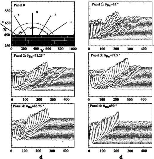
Bz versus distance through the shock front for different propagation angles, from OB• = 650 to OB• = 90 ø. For

reference, the X- Y simulation plane is plotted (panel

0) at the last time of the run •= 1.1Yci,

on which

are in-

dicated

the directions

of the slices

(straight

lines) used

for plotting the Bz profiles. The length of these slices in

panel 0 corresponds to the length "d" of the sampling

region used for the B• profiles in the other panels. In short, the well-known characteristics of a supercrit- ical perpendicular shock, i.e., the foot-ramp-overshoot- undershoot pattern, are well recovered at 0B,• = 900

(panel 5). A comparison

with ion phase

space

(not

responsible for the cyclic reformation of the shock front. This self-reformation has been already observed for a

planar quasi-perpendicular shock in 1-D [Lembdge and

Dawson, 1987] and 2-D [Lemb•ge

and Savoini, 1992]

reformation

is about < Yci >ramp. As emphasized

by

cyclic modulation

(foot and overshoot)

disappears

for

large deviations from 900 . Similar behavior is also evi- denced for the present curved shock; no cyclic reforma- tion persists for angles below OBn = 85 ø.

Several other features of a supercritical shock are well recovered in present simulations but are not detailed in the present paper. However, some quantitative results

SAVOINI AND LEMBl•GE: 2-D SIMULATION OF ELECTRON FORESHOCK Panel 850 45O 25O

0

200 400y600

800 1000

...

Figure 2. Time sequences of the local magnetic field component Bz versus distance d for different

angles of propagation 0B• from 650 (panel 1) to 900 (panel 5). Within each panel the separation

time

between

profiles

is A•- 245•. For

reference,

the location

of the shock

front

within

the

X - Y simulation plane is shown in panel 0 at a late time (t - 1.1•ci); straight lines of length d (labeled 1-5) represent the different directions (slices) along which local profiles of Bz component

are plotted in panels 1-5.

12,979

curvature effects of the shock in a self-consistent way. As expected, the magnetic field profile continuously

evolves

from a well-defined,

step-like

pattern (charac-

terized

by a narrow

thickness)

for OBn

- 90 ø, to a more

turbulent

type profile

(lying

over

a wider

space

range

in

the upstream

region)

as OBn

decreases.

A turbulent

field

The identification

and analysis

of the upstream

turbu-

shock

detailed

in the section

3.2. Such

an enhanced

up-

stream turbulence

is characteristic

of a curved

shock,

since

its level was much weaker

in 1-D and 2-D pla-

a large

deviation

angle

of the shock

normal

(OBn

- 550

from Lemb•ge

and $avoini

[1992]).

A further

compara-

required on this point.

Present

study is restricted

to the electron

foreshock,

which implies that other electron-ion foreshock mecha-

nisms

are not considered

herein. The relative

simplicity

of the present

foreshock

formation

related

to one specie

mainly (i.e., electrons)

allows

us to investigate

in detail

the basic

physical

processes

involved

into the generation

For a comparison with numerical results it is useful to summarize briefly the characteristics of the electron

foreshock as observed in the experimental data. Obser- vations have confirmed many of the basic features of the

electron

foreshock

which

were

observed

or predicted

ear-

lier (Filbert

end Kellogg

[1979]

for a first global

picture;

Ogilvie

et el. [1971],

Feldmen

et el. [1973];

Anderson

I1981],

Fitzenreiter

et el. [1984,

1990,

1996];

Yin et el.

[1998a],

Klimes

I1985],

Onseger

end Thomsen

I1991]

and Fitzenreiter [1995] for reviews and the references

inside). Figure

3 [from

Fitzenreiter

et el., 1990]

is a

12,980 SAVOINI AND LEMBgGE' 2-D SIMULATION OF ELECTRON FORESHOCK Panel 1 • 51- 22i31:30 ' .I. _ . o16 -17 -- ...=*. ß , -•" - /'i'", ß 3; -•s- / ß ,.. ß o .2o- i i ' ',,,. : '.. <.0 -2;I r• -22 - '

"- -23

--

::>'

-24

-

/

i

ß

-=s!'- ./"

i

"..

.301-7_1

I _1 •._1. I. I I ½.

ß

ß

i•....24

-25 ,./"'

.;, of ,-. ..,•

:3•:07"

:' ,:':'•

ß

"'

o•..io •'o

ß .*

Figure 3. Local electron distribution measured by ISEE satellite when crossing the edge of the

electron foreshock from [Fitzenreiter et al., 1990]. Panels 1 and 6 correspond to measurements

made in the solar wind, while panels 2-5 are for measurements at different distances within the foreshock. Panel 4 corresponds to a measurement made deeply within the foreshock.

tion measured by ISEE 1 from the solar wind (panels 1

and 6) into the electron

foreshock

(panels

2-5).

Near the leading edge of the foreshock, only electrons with high parallel velocities succeed to reach the up- stream observation point. Other electrons with lower parallel velocity are swept downstream further from the

leading edge by the incident solar wind flow. As a re- sult, a secondary peak in the parallel electron distri-

bution function is well observed when approaching the

leading

edge of the foreshock

(panel 2). The resulting

bump-on-tail distribution function is characteristic of

SAVOINI AND LEMB•GE' 2-D SIMULATION OF ELECTRON FORESHOCK 12,981

plasma wave emission associated with the electrostatic turbulence observed in the foreshock. In particular, beam-like streaming electrons have been shown to drive Langmuir-like waves near the local electron plasma fre- quency, which can be coupled to produce electromag-

netic radiation

near fp• and 2 fp• [Fredericks

et al., 1971;

Scarf et al., 1971; Canu, 1989, 1990; Bale et al., 1997; Cairns and Robinson, 1997; Cairns et al., 1997; Kasaba et al., 1997; Schriver et al., 1997; Yin et al., 1998b;

Cairns and Robinson, 1999]. Deeper in the foreshock (less energetic), electrons escaping from the shock front

do have less time to propagate far upstream, and the bump moves downward in parallel velocity until it dis-

appears in the core of the distribution (panels 3 and 4). A deeper insight of Figure 3 suggests that two dif-

ferent populations may contribute to the local distri-

bution function: a loss cone pattern (well evidenced at a certain distance from the leading edge) and a bump-

in-tail pattern for high parallel energy electrons. All

these characteristics of the Earth's electron foreshock

have to be fully recovered in present 2-D self-consistent

simulations.

The following procedure has been used for identifying the electron foreshock in our 2-D simulations, without any ad hoc assumption. One important step consists in determining as precisely as possible the energetic elec- tron population backstreaming upstream away from the shock front. For so doing, three selection criteria have

been used: (1) Electrons have to be. upstream of the shock front at the end of the run; (2) these must have

interacted with the shock front during the runtime and

(3) during this interaction, these are supposed to have

gained enough energy to be differentiated from back- ground ambient electrons. For the purpose of clarity these criteria may be presented in terms of two main

successive conditions:

1. The first condition is the selection in loca-

tion. First, at a late time of the run (herein, 1.17ci), one

selects all electrons which are located upstream of the shock without any other a priori assumption. This elec- tron population includes both all backstreaming elec-

trons which have suffered reflection with the shock front

at previous times and electrons located upstream to the shock front which did not yet interact with the shock front at that time. Second, among this population we select only those which are located in the area swept by the shock front during the simulation from an early time. This procedure eliminates all upstream electrons which did not yet interact with the shock front from this early ti. me to late time 1.1•ci.

2. The second condition is the selection in en-

ergy. One selects only those electrons which have gained enough kinetic energy in the acceleration pro-

cesses to reach at least six times the initial thermal en-

ergy Etherreal -- 0.135.

The advantage of the present method is to eliminate

safely electrons which do not have high contrast with respect to the background solar wind distribution, i.e.,

having a kinetic energy Ek < 0.8. Some electrons con-

tributing to the foreshock but having energy less than

that imposed by the second criteria may be not selected.

However, such a selection turns out to be safe enough to consider all selected electrons as the foreshock com-

ponent, independently of their locations within the up-

stream region and/or of the energization processes re- sponsible for their energetic backstreaming.

3.3. Identification of the Electron Foreshock

Location

Figure 4a plots the locations of selected electrons at

the end of the simulation (t - 1.1•ci). As reference,

the curved shock front is plotted in the X-Y simulation

x

8oo

Y

x

Y

Figure 4. (a) Locations of foreshock electrons within

the simulation

plane at time •'- 1.1Yci.

All these

elec-

trons are selected by both criteria used herein versus

locations

and kinetic

energy,

respectively

(to see text),

and the electrons are located upstream of the bow shock and within the edge of the foreshock. This foreshock

limit fits quite well with the projected

magnetic

field

line tangent

to the curved

front (thick dashed

line).

(b) Sketch

showing

the foreshock

region

sampled

with

25 boxes

(mainly aligned

along

the projected

magnetic

12,982 SAVOINI AND LEMBI•GE: 2-D SIMULATION OF ELECTRON FORESHOCK

plane with the projected magnetic field line tangent to the bow shock, which defines the leading edge of the foreshock. Several important points may be stressed: First, all selected electrons are well located within the upstream region of the shock front and downstream to the tangent line. These characteristics fit quite well with the expected location of the electron foreshock. Second, these also confirm that high-energy electrons can be detected only within a restricted area upstream to the shock front. Third, as predicted by the theory, the density of selected electrons decreases drastically as OBn increases to 90 ø. Only a few electrons are present when approaching the tangent line, in agreement both

with theory [Filbert and Kellogg, 1979; Cairns, 1987; Wu, 1984; Leroy and Mangehey, 1984] and experimen- tal observations [Anderson et al., 1979; Feldman et al., 1983; Fitzenreiter et al., 1990]. The total number of backstreaming selected electrons represents m 1% of

the total number of the "incident" solar wind particles. However, let us note that this value does not represent strictly the real percentage of foreshock electrons, since some of these may be eliminated by the selection criteria

used herein.

As evidenced in Figure 4a, no backstreaming elec- trons can be observed at the leading edge of the fore-

shock (m 90ø). This lack of particles can be due to

either the physical reasons at the leading edge or the limited number of particles per cell used in the simu- lation. This particular region will be studied in more details by using a much higher number of particles per

cell and/or by limiting the angle range of 0Br, around

900 only, instead of 650 - 90 ø.

In order to analyze in detail the dynamics of back- streaming electrons, the overall foreshock area is di- vided into 25 small sampling boxes within which lo- cal electron distributions are computed. The extent of the whole upstream sampling region is restricted to limits where backstreaming electrons have been iden-

tified (Figure 4a is used as a reference). The size of

each small sampling box has been chosen so that it is

small enough to follow the progressive changes in lo- cal distributions (both in local angle 0s,• and in dis- tance with respect to the shock front) but large enough to satisfy some reasonable statistics. Shape and lo- cations of sampling boxes are aligned along the mag- netic field lines projected within the simulation plane

as shown in Figure 4b. This disposal allows one to

keep roughly the same size for all sampling boxes in order to reproduce a constant sampling rate performed

in real satellite measurements. Then, five main different

directions of sampling have been analyzed correspond-

ing to boxes located nearest to the curved shock front

(used as reference

boxes);

more precisely,

these direc-

tions pass through the middle of the boxes. These cor-

respond to directions 0St, m 900 (near the edge of the foreshock), 83.750 , 77.50 , 71.250 , and 650 , respectively, these are defined by boxes numbered 0, 5, 10, 15, and

20. Before presenting results on local distribution func-

tions, it is important to check whether time-of-flight

frame.

3.4. Time of Flight Effects

Before comparing the numerical results with experi- mental data, it is worth pointing out that the time-of-

flight effect described in the literature [Asbr{dg½ ½! cd.,

1968; Filbert and Kellogg, 1979; Cairns, 1987; Fitzenre-

iter et al., 1990] is fully included in the present simula-

tion as illustrated in Figure 5.

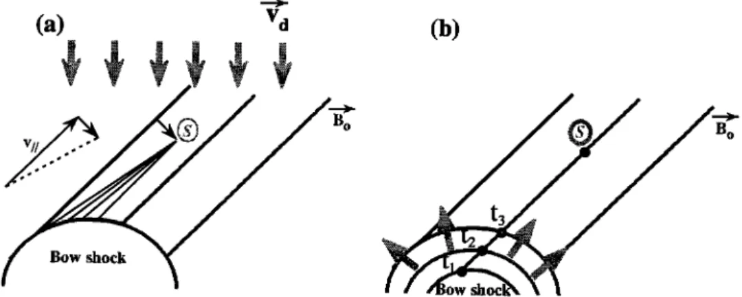
The time-of-flight effect is an important feature of

the foreshock and can be understood as a ballistic ef-

fect which is mainly due to the convection of the up- stream magnetic field lines by the incoming solar wind which carries away the backstreaming electrons into

the deeper region of the foreshock (Figure 5a). As a

result, backstreaming electrons measured farther from the shock front come from different parts of the curved shock depending on their respective parallel velocity.

Fast electrons come from the field line connected di-

rectly from the nearest point of the curved shock to

(a)

Bow shock

(b)

Figure 5. Sketch

illustrating

the comparison

of time-of-flight

effects

in (a) observational

results

and (b) present

numerical

simulations.

"S"

indicates

the location

of an observer

within the fore-

shock

region. For reference,

straight lines represent

the projection

of the magnetic

field lines

SAVOINI AND LEMB•GE' 2-D SIMULATION OF ELECTRON FORESHOCK 12,983

the observer location (S point), while slower electrons come from field lines connected from other parts of the curved shock to this S point. Then, the electron distri- bution function measured locally by a spacecraft in the upstream region includes electrons coming from differ- ent parts of the curved shock characterized by different OB• propagation angles.

In the solar wind frame (i.e., frame of the present simulation) an equivalent situation is obtained as a

given magnetic field line connected from the expanding curved shock to the observer point S will scan different angles OBn in time, as illustrated by the shock normal

directions at points •, •2, and •3 (see Figure 5b). Then, a direct comparison between experimental and numer- ical distributions can be performed and is reported in Figures 6, 8, 9, and 10.

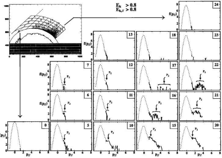
4. Local Electron Distribution Function

Local distribution functions can be computed in the different sampling boxes by superimposing Figure 4b onto Figure 4a. It clearly appears that distribution functions cannot be measured accurately along the edge

of the foreshock (boxes 1, 2, 3, 4, 8, and 9) and too far from the shock front (boxes 14-19), since the number of selected electrons is too low (or even null).

4.1. Total Distribution and Back-streaming

Electron Distribution

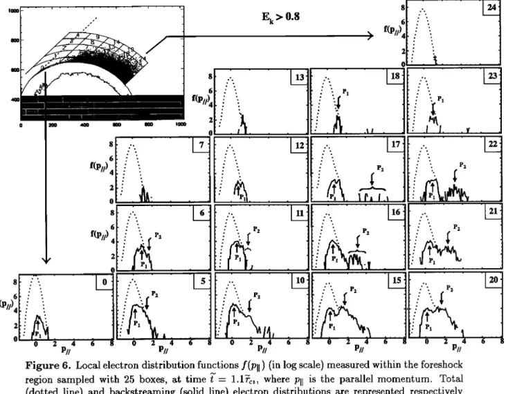
Reduced

parallel

f(Pll) distributions

calculated

from

f(PlI,P•-) are reported

in Figure

6. Within each

box,

both the total distribution, hereinafter

noted ft (in-

the Back-streaming electrons' distribution, hereinafter noted lb, are plotted. Let us note that the dotted line

(representing the total distribution) is mixed with the solid line (representing the Back-streaming electrons)

in the high-velocity range since it involves these ener- getic electrons. The comparison between Figures 3 and 6 shows a very good qualitative agreement with experi- mental data, which can be summarized as follows: The

total parallel

distribution

ft(pll

) (dotted

line) exhibits

a

characteristic bump-on-tail pattern observed in-situ in the different sampling boxes. For the purpose of clar- ity, we will analyze local distributions, first, versus pro- gressive deviation from 90 ø and for boxes nearest to the curved shock front, and, second, versus relative distance

from the shock front.

4.1.1. Variation versus angle. Sampling boxes

versus angle near the shock front allow one to stress the following features:

1. In the vicinity of the leading edge (box 0), Back-

streaming electrons have still low energy and are imbed- ded within the main core of the upstream undisturbed distribution; in addition, the number of these electrons

is weak. These form a relatively cold (narrow) popula-

tion animated with an averaged weak parallel drift ve-

locity. No bump-in-tail pattern (or cold electron beam pattern) can be evidenced too near the leading edge of

the foreshock.

However, for more oblique direction, the bump pat- tern is clearly identified and is even amplified quite well

for large deviations from 90 ø (boxes 5, 10, 15 and 20). This is in contrast with the fact that it is expected to disappear more deeply within the foreshock. Such a dis- crepancy may be explained by remembering that more

oblique direction (i.e., measurements made presently very near the curved shock front) should not be con-

fused with measurements made more deeply within the foreshock as mentioned in experimental works. Such

last measurements include also variation in distance

with respect to the shock front itself, a fact which can be reproduced too by the present sampling measurements.

2. As angle deviates from 90 ø , the Back-streaming population has a much higher density, an increasing thermal momentum, and an increasing parallel drift mo-

mentum

< Pll >' These

electrons

mainly form a bump-

in-tail with a momentum sign opposite to that observed in experimental data, since present simulations are in the solar wind frame. The relatively narrow extent of the field-aligned suprathermal distribution in box 0 be-

comes much broader (heating) as evidenced in boxes 5, 10, 15, and 20. This feature persists also at different distances from the shock front (boxes 6, 11, 16, and 21). Such a broadening evidenced with further pene-

tration within the foreshock is in good agreement with

the observations of Feldman et al. [1983].

3. Two different population components can be clearly identified in the Back-streaming population. When deviating from the leading edge of the foreshock,

the well-pronounced, single-peaked distribution (P• in boxes 0 and 5) is progressively replaced by a double- peaked distribution (P• and P2 in boxes 10, 15, and 20). This change has two consequences: First, this sug-

gests the necessity for analyzing separately high and

low parallel energetic electrons (as already mentioned for experimental results of Figure 3). This point will

be developed in section 4.2. Second, with more oblique deviation, electrons of peak P2 depart from the distri- bution tail and are responsible for the formation of a bump-in-tail around a finite-averaged parallel drift mo- mentum. For large deviation from 900 this drift in-

creases

and reaches

a maximum

value < Pll >• 1.5

becomes partially filled in (box 20).

In summary, these results can be interpreted as a progressive transformation of the bulk energy of Back- streaming electrons into thermal energy as the direction

with the shock normal is strongly oblique (boxes 5, 10, 15, and 20). Such features can be understood if one con-

siders that electrons located around the leading edge of

12,984 SAVOINI AND LEMB•GE' 2-D SIMULATION OF ELECTRON FORESHOCK

0.8

f(P/)

! ,

-17!

'1 51

ß

f(P//)4

118: ....

[23:

ß i P1

: .1•1. . v .

ß ' . . -122:

' ' :'

'".

' r2' '[

211

i •

. . .

,11[

__

t'[/i. __.

Figure 6. Local

electron

distribution

functions

f(Pll) (in log scale)

measured

within

the foreshock

region

sampled

with 25 boxes,

at time t - 1.1'rci,

where

Pll is the parallel

momentum.

Total

(dotted line) and backstreaming

(solid line) electron

distributions

are represented

respectively

locations of the curved shock front, of the backstreaming electrons, and of the sampling boxes

within the simulation

plane (see

also

Figure

4b for precise

labels

of sampling

boxes);

the foreshock

edge

is illustrated

by the projected

magnetic

field line tangent

to the curved

front (dashed

line)

fiected (and accelerated) more recently than those of

other groups. As a consequence, these did not have enough time to interact with the ambient solar wind plasma; this is in agreement with the absence of up-

stream turbulence observed as OB, approaches 900 (see Figure 2). Then, results of boxes 0, 5, or 6 can be con- sidered as characteristic distribution functions just after the reflection process and before driving various elec- trostatic and electromagnetic instabilities. In contrast, electrons of boxes located at more oblique angles have left the shock front much before those of boxes 0, 5, and 6 and have enough time to trigger some instabilities. As a consequence, these fluctuations cause some diffusion

in energy (and in pitch angle) as shown in boxes 10,

15, and 20 and 11, 16, and 21. This behavior seems to be well confirmed by the presence of upstream electro- static and electromagnetic wave activity evidenced for

0e• _< 77.50 (Figure 2).

4.1.2. Variation versus distance. Let us con-

sider the direction centered around the projected field

line starting from the curved shock front at 0B, m 65 ø.

Results clearly show that the bump-in-tail (box 20) is

progressively replaced by a well-pronounced beam pat-

tern (separated

from the main distribution)

as the dis-

other words, the parallel drift of high-energy electrons

(peak P2) strongly increases, that is, only the most en-

ergetic electrons can be observed at large distances from the shock front, but their density decreases rapidly with distance, and no field-aligned beam pattern can be iden-

tified too far from the front (box 24). As 0B• increases

to 90 o , the beam pattern can be partially identified over much shorter distances from the front, which can explain the difficulty for evidencing clearly such a lo- cal feature in experimental data. Similarly, low-energy

electrons also suffer an increasing parallel drift (peak P•) as the distance from both the foreshock edge and

the bow shock increases. As a consequence, two differ- ent bump-in-tail patterns may be identified in the total

distribution

ft(pll

) at different

locations

where

mecha-

SAVOINI AND LEMB•GE' 2-D SIMULATION OF ELECTRON FORESHOCK 12,985 nisms of formation largely differ; both patterns result

from time-of-flight effects.

A relatively narrow bump-in-tail pattern is pres- ent both for large deviations from the leading edge of the foreshock and large angle; it is mainly due to the

contribution of shifted peak P• (as in boxes 18 and 23).

Such a distribution can also be observed for short de-

viation and nearer to the shock front (see boxes 6 and

In contrast, for any oblique deviations from 900 but very near of the shock front, a much broadened bump- in-tail pattern is evidenced; it is only due to the con-

tribution of the shifted peak Pa (boxes 5, 10, 15, and 20). However, when penetrating deeply within the fore- shock region (i.e., by combining both large deviations and large distance from the shock front), the resulting wide bump-in-tail pattern tends to be much narrower until being smoothed out within the total distribution for two combined reasons: absence of high-energy elec-

trons (no Pa peak) and finite parallel drift of low-energy electrons (i.e., peak P•). These results illustrate the

progressive disappearance of the bump-in-tail pattern to be compared with that evidenced in experimental

data as detailed in section 5.

Unlike the parallel distribution, the perpendicular

distribution ft(pñ) (not shown herein) exhibits a fiat-

top pattern which enlarges the tails of the incoming

Maxwellian distribution. This feature is almost un-

changed for any direction and almost any distance from the shock front. However, a loss cone type pattern ap- pears at small oblique deviations from 90ø; this will be analyzed in more details in section 4.2. At a large de-

viation from 90 ø, the only change in ft(p_k) is a slight

decrease in the width of the fiat-top distribution, as the

distance from the curved shock front increases.

4.2. Low and High Parallel Energy

Distributions

Until now, we have only analyzed the behavior of Back-streaming electrons according to their locations.

Both experimental (Figure 3) and present numerical re- sults (Figure 6a) emphasize differencies in the parallel

distribution function which suggest that one perform a more detailed investigation of local distributions versus the level of parallel kinetic energy.

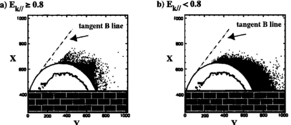
We have separated all selected Back-streaming elec-

trons (Figure 4a) into two groups, with parallel kinetic

energy

Ekl[ higher

and lower

than 0.8. Locations

of se-

lected electrons are shown in Figures 7a and 7b, respec-

tively. This selection

in Ekll corresponds

to momentum

value Iplll • 1.2, where

peak Pa departs

clearly

from

the tail of ft(Pll) in box 10 of Figure

6. This procedure

allows one to identify more clearly the characteristics of electrons contributing to peaks P• and Pa. It is im- portant to stress that this selection does not invoke any assumption on the perpendicular velocity component.

Again, one applies a spatial distribution

of sampling

boxes

within the foreshock

region

(from boxes

1 to 24)

Figure 7 shows that results obtained in section 4.1

still persist for each separate population. First, density

of each population strongly increases as 0B• decreases from 90 o to 65 ø. Second, each population exhibits an

effective limit near the foreshock edge along which den-

sity is almost null. However, important differences are evidenced between both populations and are summa-

rized as follows:

4.2.1. Case E•i I > 0.8 (Figures 7a and 8). High

The spatial distribution of these electrons is not homo- geneous. These strongly accumulate along the projec-

tion of the magnetic field Bo in the simulation plane

(Figure 7a), which corresponds

to the extreme

region

tail in the total distribution

ft(Pll

) at short

distances

a) Ek//_>

0.8

/ tangent

B line

///•

/,

'..

b) Ek//< 0.8

/ tangent

B line

Figure 7. Locations of foreshock electrons within the simulation plane at time t - 1.1Y•i, for (a) high parallel kinetic energy and (b) low parallel kinetic energy. The foreshock edge is illustrated by the projected magnetic field line tangent to the curved front (dashed line).

12,986 SAVOINI AND LEMB•GE: 2-D SIMULATION OF ELECTRON FORESHOCK ... Ek > 0.8

Ek,// > 0.8

-

....

...

8 :....

7 •

f(P//)

4

' P2

2

0. . itt: .

.

•

f(p//)6

p//

p//4

p//4

Figure 8. Figure similar to Figure 6 for backstreaming electrons selected with high parallel kinetic energy

/high(p_t_)

(not shown

herein)

does

not exhibit

any loss

flat-top-like pattern as both propagation angle becomes more oblique and the distance increases from the shock

front.

The absence of loss cone structure in the perpendic- ular distribution suggests different possibilities, which

can be summarized as follow:

1. The reflection process for this population is not a mirror reflection, and another reflection mechanism has to be invoked to explain the observation of this high parallel energy electron component. One expla- nation is that electrons penetrate the shock front and find conditions for spending some time to interact with local macroscopic fields. Since the shock front is nonsta- tionary and non-homogeneous, these may find some ap- propriate conditions to be reinjected upstream at later times and to escape with some energy high enough to be selected in the electron foreshock population.

2. The reflection process is a mirror reflection, and wave scattering destroys the loss cone signature until producing a Gaussian perpendicular distribution

function. Absence of loss cone evidenced in our results

almost everywhere could suggest a very efficient and

rapid, local wave-particle scattering process. However, such a process has not enough time to produce a Gaus- sian shape as compared to the short time of electrons escaping from the front and propagating upstream along

the magnetic field lines (formation of field-aligned beam or bump-in-tail even very close to the shock front). Nev-

ertheless, the precise impact of the high wave activ- ity observed upstream of the shock front on mirrored- reflected electrons has not been analyzed in details yet.

3. High-energy Back-streaming electrons corre-

spond to leaked electrons (originating from the down- stream region) which fill up the loss cone distribution (herein Px population). Indeed, electron leakage from

the magnetosheath region has been invoked in previous

works but seems not to be important [Fitzenreiter et al., 1990]. One simplified approach to check this possibility

is that after interacting locally with downstream waves, leaked electrons are supposed to have enough parallel energy to be able to overcome the electrostatic barrier

in order to cross back the shock front from downstream

to upstream region. By assuming that adiabatic invari- ant is conserved ,through the shock crossing, one ex- pects that the perpendicular downstream temperature will be lower than its upstream value. For so doing, local distribution function has been calculated in sampling

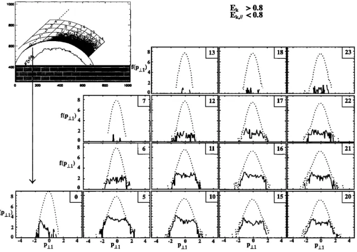
SAVOINI AND LEMB•GE: 2-D SIMULATION OF ELECTRON FORESHOCK 12,987 Ek > 0.8

Ek,// < 0.8

.... I'-_

.... I ....

f(P.l_l)

4

f(P-I-1)

4

f(P.t.1)4

Figure 9a. Figure

similar

to Figure

6 for perpendicular

distributions

flow

(p•_•)

of backstreaming

electrons selected with low parallel kinetic energy only, where p•_• is the perpendicular momentum

component (direction defined in Figure lb).

boxes

extended

from upstream

(subscript

"u") to down-

P2 population

only) and Tll,,

, respectively.

Results

show

that T•_•/Tll,• = 0.9, which contradicts

conservation

not support a leakage process from the magnetosheath as being dominant, since it does not account for the

perpendicular distribution of the high-energy P2 pop-

ulation; rather, this result supports that wave-particle

scattering (upstream turbulence) may contribute to this population.

A more rigorous approach is necessary, and all three

possibilities can be fully analyzed by following the time

histories of reflected electrons; this work is lefSt for a further study. At the present time, the respective con-

tribution of the two main dominant processes invoked

herein, namely, acceleration by macroscopic fields at the

shock front and wave-particle scattering by upstream

turbulence, is not yet determined.

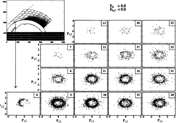
4.2.2. Case

E•l

I < 0.8 (Figures

7b and 9). The

behavior of low parallel kinetic energy electrons is corn-

pletely different, which means that different reflection mechanisms must be invoked. This population forms

the main part of the fb population

(m 74%). In con-

trast with the previous

population

(Figure

7a), the spa-

more homogeneous

(Figure 7b) throughout

the whole

strongly

increases,

as OBr•

decreases

from 900 to 65ø).

tion function

floW(Pll)

correspond

to those

of peak

P•

(Figure 6) discussed in section 4.1.

Complementary

information

is obtained

in studying

the perpendicular component of the distribution func-

tion fløW(p_c)

represented

in Figure

9a. The striking

feature is the evidence of a characteristic loss cone sig-

nature. It is important to remember that no selection

criteria has been used on the perpendicular

velocity

component; in other words, such a pattern is the con- sequence of a real process. This allows us to claim that

magnetic

reflection

process

is the main source

of the

energization for this population. As is well known and

described by the theory, magnetic reflection is respon- sible for loss-cone signature by selecting the most en-