HAL Id: hal-00316178
https://hal.archives-ouvertes.fr/hal-00316178
Submitted on 1 Jan 1997
HAL is a multi-disciplinary open access
archive for the deposit and dissemination of sci-entific research documents, whether they are pub-lished or not. The documents may come from teaching and research institutions in France or abroad, or from public or private research centers.
L’archive ouverte pluridisciplinaire HAL, est destinée au dépôt et à la diffusion de documents scientifiques de niveau recherche, publiés ou non, émanant des établissements d’enseignement et de recherche français ou étrangers, des laboratoires publics ou privés.
Model results for the ionospheric E region: solar and
seasonal changes
J. E. Titheridge
To cite this version:
J. E. Titheridge. Model results for the ionospheric E region: solar and seasonal changes. Annales Geophysicae, European Geosciences Union, 1997, 15 (1), pp.63-78. �hal-00316178�
Ann. Geophysicae 15, 63—78 (1997) ( EGS — Springer-Verlag 1997
Model results for the ionospheric E region: solar and seasonal changes
J. E. TitheridgeInstitute for Meteorology & Geophysics, University of Graz, Halba¨rthgasse 1, A-8010 Graz, Austria* Received: 22 January 1996/Revised: 26 June 1996/Accepted: 22 July 1996
Abstract. A new, empirical model for NO densities is developed, to include physically reasonable variations with local time, season, latitude and solar cycle. Model calculations making full allowance for secondary produc-tion, and ionising radiations at wavelengths down to 25 As , then give values for the peak density NmE that are only 6% below the empirical IRI values for summer conditions at solar minimum. At solar maximum the difference in-creases to 16%. Solar-cycle changes in the EUVAC radi-ation model seem insufficient to explain the observed changes in NmE, with any reasonable modifications to current atmospheric constants. Hinteregger radiations give the correct change, with results that are just 2% below the IRI values throughout the solar cycle, but give too little ionisation in the E-F valley region. To match the observed solar increase in NmE, the high-flux reference spectrum in the EUVAC model needs an overall increase of about 20% (or 33% if the change is confined to the less well defined radiations atj(150 As). Observed values of
NmE show a seasonal anomaly, at mid-latitudes, with
densities about 10% higher in winter than in summer (for a constant solar zenith angle). Composition changes in the MSIS86 atmospheric model produce a summer-to-winter change in NmE of about !2% in the northern hemi-sphere, and #3% in the southern hemisphere. Seasonal changes in NO produce an additional increase of about 5% in winter, near solar minimum, to give an overall seasonal anomaly of 8% in the southern hemisphere. Near solar maximum, reported NO densities suggest a much smaller seasonal change that is insufficient to produce any winter increase in NmE. Other mechanisms, such as the effects of winds or electric fields, seem inadequate to explain the observed change in NmE. It therefore seems possible that current satellite data may underestimate the mean seasonal variation in NO near solar maximum. A not unreasonable change in the data, to give the same 2:1 variation as at solar minimum, can produce a seasonal
* Permanent address: Physics Department, The University of
Auckland, Auckland, New Zealand
Correspondence to: J. E. Titheridge
anomaly in NmE that accounts for 35—70% of the ob-served effect at all times.
1 Introduction
In recent years it has become possible to model, with reasonable accuracy, most of the processes involved in the formation of the ionosphere. The physics involved is parti-cularly straightforward for the ionospheric E region, where the ionisation time-constant is only a few minutes, so that conditions are always close to equilibrium. Move-ment effects are also small, because of the short time-constants, so that changes due to diffusion, winds and electric fields are of minor importance. Model calculations are then reasonably straightforward. Results obtained for the peak density NmE are, however, commonly about 30% below observed values, while the calculated width and depth of the valley between the E and F1 regions are perhaps two times too large (e.g. Titheridge, 1990; Buon-santo, 1990; Buonsanto et al., 1992; Tobiska, 1993). Be-cause of the square-law loss process, an increase of 40% in
NmE requires an increase of 100% in the ionisation rate at
the peak of the E layer (at 105—110 km). To reduce the size and depth of the valley requires an even larger increase in production at heights of 120—150 km.
In a previous paper (Titheridge, 1996), production rates were calculated using a new approach to determine the total amount of secondary ionisation, based directly on the energy of the incoming photons. This procedure auto-matically makes full allowance for changes in the EUV spectrum and in the photo ionisation cross-sections. It gives an increase of up to 20% in values of NmE calculated using the newer radiation models which have increased fluxes at short wavelengths. The EUV models commonly used for ionospheric calculations extend down to a wavelength of 50 As , with all radiations between 50—100 As included in a single band. Subdividing this band, and including radiations down to 25 As , gives a fur-ther increase of 8—10% in NmE, so that final values are now only 12% below mean experimental results for equi-nox conditions at F10.7"110.
Ionospheric models are particularly valuable for inves-tigating the changes that would result, in observed quant-ities, from changes in individual input parameters. In the present work a study is made of the changes in NmE with season and with solar cycle, caused by changes in current models of the solar EUV radiation and in the composition of the neutral atmosphere. For this purpose, a new model for the density of NO in the upper atmosphere is de-scribed. This uses recent data from the Solar Mesosphere Explorer (SME) satellite to construct an empirical model that has reasonable variations with season, latitude, solar cycle and time of day. NO is produced by solar radiation, giving increased densities in summer that lead to an in-crease in loss rates for O`
2 ions in the E region. It therefore seemed that changes in NO might explain some of the observed seasonal anomaly in the E region — where values of NmE are about 10% larger in winter than in summer, for mid-latitude conditions at a constant solar zenith angle.
Model calculations are also used to see whether the solar variations in current EUV flux models are compat-ible with observed changes in the ionosphere. For this purpose we assume that solar-cycle changes in the neutral atmosphere are correctly defined by the MSIS86 atmo-spheric model (Hedin, 1987). Results suggest that, even if the normal increase of NO near solar maximum is sup-pressed, the EUVAC model as it stands cannot give a suf-ficiently fast increase in E-region densities during the solar cycle. The earlier Hinteregger model, however, gives a rate of change that closely matches the observations.
For comparisons with experimental data, use is made of results incorporated in the International Reference Ionosphere model IRI-90 (Bilitza, 1990). This model uses analytic expressions that have been fitted to a large amount of monthly median data, to best reproduce mean observed values of ion density at different heights. In particular, it gives values of NmE corresponding to the results obtained by Kouris and Muggleton (1973a, b) from an extended study of monthly median values of foE, for each hour between 0900 and 1500, from 45 sites spaced around the globe, and covering a full 11-year solar cycle.
2 The modelling program
The general features of the modelling program have been described previously (Titheridge, 1993). The densities of O, O2, N, N2 and H are obtained from the MSIS86 atmospheric model (Hedin, 1987). Ion chemistry includes all the reactions normally considered (e.g. Buonsanto
et al., 1992) plus four further charge-exchange reactions
involving NO: N`
2#NOPNO`#N2 O`(4S)#NOPNO`#O N`#NOPNO`#O O`(2P)#N2PN`#NO and five metastable decay processes:
O`(2D)PO`(4S)#hl O`(2D)#N2 PO`(4S)#N2 O`(2P)PO`(4S)#hl O`(2P)#ePO`(4S)#e O`(2P)PO`(2D)#hl.
Allowance is made for the direct production of N` ions, through ionisation of N2 or of N, since this is significant under some conditions. H` calculations are included, along with a full allowance for the effects of diffusion, winds, exospheric fluxes and temperature gradi-ents (as summarised by Titheridge, 1993) to ensure a real-istic F-layer as the upper bound of the valley region.
The total number of ions that are produced by one photon depends mainly on the energy of the photon. This dependence has been used to construct a simple scheme for obtaining a close approximation to the total ion pro-duction under a wide variety of conditions (Titheridge, 1996). Unlike traditional methods, which determine the bidirectional photoelectron flux as a function of height, calculations based on the overall energy distribution work well at all heights down through the lower E region. Compared with earlier calculations using a fixed correc-tion of 30%, inclusion of a full allowance for secondary production gives an increase of about 20% in calculated densities at the peak of the E-layer. The increase is even larger at heights above the peak of the layer, so that the size of the E-F1 valley is appreciably reduced.
For most calculations EUV intensities are taken from the recent EUVAC model (Richards et al., 1994), which uses linear interpolation between reference spectra at
F10.7"80 and 200. The intensities are specified in 37
wavelength bands covering the range from 50 to 1050 As , as used in many studies (e.g. Torr and Torr, 1985). In the present work two changes are made to this scheme. First-ly, the normal band 1 (from 50—100 As ) is divided into smaller sections. This is necessary for accurate profile calculations at heights below 150 km, because of the large number of secondary electrons produced by high-energy photons. As the wavelength decreases from 100 to 50 As , the mean number of secondary ions produced per photon increases from about 2.1 to 4.4, while the height of maximum production decreases by about 9 km (Titheridge, 1996). To reproduce these changes correctly, and to include the secondary ionisation produced by high-energy photons in the range 25—50 As , the normal band 1 is replaced by four bands covering 25—40, 40—60, 60—80 and 80—100 As . Photoionisation cross-sections for these bands are obtained from the detailed data of Fenelly and Torr (1992), as described in Titheridge (1996).
The second change to the commonly used EUV spec-trum is the addition of a band to include the strong Lya radiation at 1216 As . This radiation produces NO` ions only, and is the major source of ionisation at heights below 95 km. Direct ionisation of NO by Lya also in-creases total ionisation rates by about 2% in the daytime E region. At night, scattered Lya provides up to 30% of the total ionisation at heights near 130 km.
3 An empirical model for the NO layer
3.1 The production and loss of NO
At low and mid-latitudes, NO is produced primarily as a result of daytime photoionisation. Direct or indirect dissociation of N2, by solar photons and secondary
electrons, produces excited N(2D) atoms which react with O2 to produce NO. The normal ground state N(4S) can also produce NO, but the rate constant for this reaction is slower by a factor of over 10000 at heights below 120 km (Rusch et al., 1991; Torr et al., 1995). So in the E region, production of NO is important only during the day.
Loss of NO is mainly through its reaction with N(4S), particularly at night when the densities of N(2D) and O` 2 are greatly reduced (e.g. Torr et al., 1995). In the E and F1 regions the density of N(4S) increases with height, giving increasing loss rates. This produces a well-defined NO layer with a peak near 110 km. We should note that N(4S) densities are not well defined at heights below 200 km, where data are very sparse and the variations in the MSIS86 model are guided largely by theory. Theoretical calculations of NO densities based on this data do, how-ever, provide a good match with AE-C measurements over the height range 130—250 km (Rusch et al., 1991).
At 120 km the density of N(4S) is about 2.0]106 cm~3 near noon, giving a time-constant of 4 h for the loss of NO. The time-constant drops to 1.6 h at a height of 130 km, and 0.8 h at 140 km, as the density of N(4S) increases (with a peak near 190 km). N(4S) densities are approximately halved at night, causing the time-constants to increase by a factor of about 2 after midnight. Night-time recombination with a mean Night-time-constant of around 6 h (at 120 km) should cause NO densities to decrease by a factor of 5—10, reaching a minimum just before dawn. Mean daytime densities should follow the latitudinal, sea-sonal and solar-cycle changes in the solar irradiance, at low and mid-latitudes. Current results suggest an increase by a factor of about 2 from winter to summer, at latitudes of 25°—40° near solar minimum (e.g. Stewart and Cravens, 1978; Ge´rard and Noe¨l, 1986). This is sufficient to make appreciable changes to the E-region ionisation.
At high latitudes there is a large production of N(2D) by electron impact in the auroral regions. The resulting production of NO is larger and more variable than at low latitudes, with little diurnal variation and only a small solar-cycle change. NO densities will increase, and extend to lower latitudes, with increases in magnetic activity; this could have produced the apparent increase in mid-lati-tude densities in winter, found in some early studies. Even under quiet conditions the data of Fesen et al. (1990) show day-to-day variations of up to about $20% in NO dens-ities at latitudes below 45°, and twice this at higher latit-udes.
3.2 Daytime densities, as a function of solar activity
Published studies suggest that from solar minimum to solar maximum the daytime NO densities, at low lati-tudes, increase by a factor of about 3.5 (Kuze and Ogawa, 1988; Ge´rard et al., 1993); 3—4 (Ge´rard et al., 1990); 4—5 (Fesen et al., 1990); 7 (Fuller-Rowell, 1993); and 7.5 (Barth
et al., 1988). Seasonal and latitudinal variations, in the
daytime thermosphere, are shown best in the work of Fesen et al. (1990). This uses data from the Solar Me-sosphere Explorer satellite at local times near 1500 LT, close to the diurnal maximum in NO. Mean variations
Fig. 1a, b. Mean values of NO a at the equator and b at latitudes of 30°N and 30°S, for the months of March, June, September and December of each year from 1982 to 1985. Each point gives a mean value for the peak density, at heights near 110 km and for a local time near 1500 LT, from Fesen et al. (1990). All data are for magneti-cally quiet conditions. The plotted curves are obtained from Eq. 2. Dotted lines in b show a modified variation discussed in Sect. 6
with latitude are given for March, June, September and December of each year from 1982 to 1985, covering solar fluxes from about 180 to 70. Mean values for the peak density of NO, at the height of the maximum (near 110 km), are also tabulated for each month and each year at latitudes of 0°, $30° and $60°.
The 16 mean values given by Fesen et al. (1990), at 0° latitude, are plotted in Fig. 1a. The data show a well-defined increase with solar activity, by a factor of about 4, for values of F10.7 increasing from 69 to 186. There is no consistent variation with month, and all data show some tendency for a decrease in *(NO)/(*F10.7) near solar maximum. The mean trend is well represented by the dotted line in Fig. 1a, which corresponds to the relation
D@"14.8#0.22(F10.7!100)
!
0.0008(F10.7!100)2]106 cm~3. (1) The most recent low-latitude data set is that used by Ge´rard et al. (1993) for comparison with model calcu-lations. These data tend to be grouped near solar fluxes of about 73, 105 and 170. Mean values were scaled for each group, giving NO densities of 8.5(8.3), 16(15.9) and 28(26)] 106 cm~3. Values in brackets are the corresponding re-sults from Eq. 1. The good agreement lends confidence in
the use of Eq. 1 to define the mean density at the peak of the NO layer, at low latitudes.
3.3 Seasonal and latitudinal changes
The mean values of NO density tabulated by Fesen et al. (1990), for latitudes of 30°N and 30°S, are plotted in Fig. 1b. Solid dots are for the summer hemisphere, and solid triangles for winter; these include all the tabulated data for June and December. Two points (at 30°S, in June 1984 and 1985) have been adjusted downwards, since they fall on the start of the rising portion of the mean plots, where the winter values increase rapidly towards the high-er auroral density (as will be discussed). The winthigh-er value at F10.7"186 has also been adjusted upwards by 10%. These changes give points that follow more accurately the trend of the central near-linear section of the mean plots in Fesen et al. (1990).
The mean summer and winter densities plotted in Fig. 1b, for a latitude of 30°, show an overall trend that is very similar to the equatorial results of Fig. 1a. The con-tinuous and broken lines correspond to the dotted curve in Fig. 1a, shifted by $3.0]106. This provides a near-optimum fit to the data for both summer (solid dots) and winter (triangles). The equinox data from Fesen et al., for March and September of each year, are shown as open symbols. These are coded according to the hemisphere, with values for March distinguished by a central dot. At medium and high levels of solar activity these equinox data (at a latitude of 30°) are reasonably well centred between the summer and winter curves. Thus they agree well with the curve of Fig. 1a, based on data from March, June, September and December at a latitude of 0°. The agreement is less good near solar minimum, but still acceptable in view of the increased scatter at this time.
The fixed difference between the three plotted curves in Fig. 1 corresponds to a fixed latitudinal gradient in the NO densities, of 0.10]106 per degree of latitude, for summer or winter. The lack of any consistent variation with month or with latitude in the equinox data (open symbols in Fig. 1b), indicates a mean gradient of zero between 30°N and 30°S for the equinox months. The combined latitudinal and seasonal change can therefore be represented by the relation
D0"14.8#0.22(F10.7!100)
!
0.0008(F10.7!100)2#0.1s· /]106 cm~3, (2) where/ is the latitude in degrees; s is a seasonal index which varies from #1 in June to 0 at the equinoxes and !1 in December, so that s"sin(0.0172[d!80]), where
d is the day number. The seasonal term gives a constant
change from winter to summer, so that the summer/winter ratio is greatly reduced near solar maximum. As discussed in Sect. 6, this does not agree well with simple physical considerations or with observed seasonal changes in NmE, and a modified form giving a constant seasonal effect might be preferable. This is obtained using Eq. 14 in place of Eq. 2, and gives the variations shown by dotted lines in Fig. 1b.
Scatter plots were also given by Fesen et al. (1990) for data in two quiet periods in each of June and December. Mean trend lines drawn through these four sets give slopes (at the equator) of 0.10, 0.09, 0.08 and 0.08] 106 cm~3 per deg latitude. The consistency of these re-sults, in spite of a 2:1 variation in the equatorial densities, supports the use of a fixed latitudinal gradient. The re-striction to quiet intervals has produced a slightly lower gradient than the value (0.1]106) obtained from the over-all mean plots, but the change is barely significant. The different plots in Fesen et al. (1990) show that this approx-imately constant gradient is observed, in most cases, at latitudes from about 30° in the winter hemisphere to 60° in summer.
3.4 A high-latitude model
In the auroral regions there is a large, additional source of NO from high-energy particle precipitation. The mean curves given by Fesen et al. show increased NO densities at latitudes above 60°, with a tendency to peak at about 75° (as also found by Ge´rard et al., 1990). For latitudes of 60°—90° most of the mean data lie between 20 and 40]106, in all years and all seasons. There is some de-pendence on solar activity, with mean values increasing from about 22 at F10.7"70 to 33 at F10.7"180 giving
DF"(15#0.1F10.7)]106 cm~3. (3) Smith et al. (1993) used data from 51 rocket flights and 36 satellite sets, to determine the mean variation of NO density with latitude, exospheric temperature and Kp. The data were primarily from latitudes near 0, 31, 39 and 60—65°N, at values of F10.7 from about 70—250. For the high-latitude group there was little diurnal variation, but a large change with magnetic activity. The changes with
Kp corresponded to a factor exp (0.40Kp) for the rocket
data, and exp (0.26Kp) for the satellite results. We will assume a mean Kp variation corresponding to exp (0.32Kp). For values of Kp up to about 5, this can be approximated quite well by a term (1#0.1Ap), where
Ap is the planetary index.The changes with solar activity were given as a factor
exp (c1¹=), where ¹= is the exospheric temperature and
c1"0.0010 for the rocket data and 0.0005 for the satellite
results. From the tables in Smith et al. we have ¹=+ 4F10.7#525 for these data. Using c1"0.0008 then gives a solar-cycle change proportional to exp (0.0032F10.7), so that NO densities increase by 52% when F10.7 changes from 100 to 230. This agrees very closely with the vari-ation DF derived from the work of Fesen et al. (1990), as shown in Fig. 2. The NO variations at high latitude are therefore defined by
DH"0.5(15#0.1F10.7)(1#0.1Ap)]106 cm~3. (4) The Fesen et al. data correspond to a median Ap of 17, so that Eq. 4 requires an initial constant of 0.37 to agree with Eq. 3. The Smith et al. data give appreciably greater NO densities, corresponding to an initial factor 0.66. The value 0.5 used in Eq. 4 is close to the geometric mean of
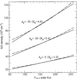
Fig. 2. Mean values for the peak NO density, at latitudes of 60—90°, as a function of solar flux and magnetic activity. Solid lines are from Eq. 4; this corresponds to the mean high-latitude results of Fesen
et al. (1990) (at Ap+17) increased by 35%. Broken lines give the
expression DNO"exp(15.91#0.0032F10.7#0.005Kp), derived from the work of Smith et al. (1993), decreased by 24%
these estimates. This high-latitude result is used to define the density at the peak of the daytime NO layer, for latitudes greater than 60° in both hemispheres.
Optimum agreement with the full set of plots given by Fesen et al. (1990) is obtained if Eq. 2 is used for latitudes of !45° to #45° in March, !30° to #50° in June, !20° to #40° in September and !50° to #30° in December. Results then reproduce, for instance, the steady increase in [NO] from !20° to !60° evident in all four of the September data sets. The present study adopts a slightly simpler procedure, with upper limits of 40° for both hemispheres in March and September. Equa-tion 2 is then used up to a latitude/M of 30° in winter, 40° in equinox and 50° in summer, given by
/M"40#10·s degrees, (5)
where s is the seasonal index from Eq. 2. This gives a symmetrical mean variation for determining average global changes.
At latitudes above 60°, peak densities are defined by Eq. 4. Intermediate latitudes use a linear interpolation between the results from Eq. 2, at a latitude/M, and the results from Eq. 4 for a latitude of 60°. This interpolation is quite smooth in summer, when Eqs. 2 and 4 give similar results at /+60°. A much larger change is involved in winter, when the data (and the change from Eq. 2 to Eq. 4) give an increase by a factor of 1.2 to 4 over a latitude range from about 30° to 60°.
3.5 Diurnal variations
Good data on the diurnal variations in NO densities are not readily available, since most satellite measurements
are restricted to daylight hours. To overcome this prob-lem, Smith et al. (1993) analyse seven rocket and six satellite values for the density at a height of 110 km. Results at the equator show an increase by a factor of 7 from the predawn minimum to the mean daytime value. This factor decreased at higher latitudes, or with increases in Kp. For a latitude of 30°, and Kp"2.5, the derived expressions give a mean day/night ratio of only 2—3. This value is supported directly by only a small number of mid-latitude rocket data, which give a mean diurnal vari-ation of about 3 : 1. The decrease with latitude seems to be caused primarily by the inclusion of data at latitudes above 60° in an overall, linear correlation. The high-latit-ude data (clustered near 65°) show no significant diurnal variation, but a high correlation with Kp — whereas the low-latitude data show a large diurnal change and no correlation with Kp.Changes in the density at the peak of the NO layer, from 0600 to 1800 LT at the equinoxes, are clearly dis-played in the results of Rusch et al. (1991). Data from the satellite Atmosphere Explorer C, at latitudes of 0°—30°, are compared with the results of a full model calculation. In both cases there is a rapid increase of NO densities from 0600 to 1000, with maximum values occurring at about 1400. For the satellite data, the increase from 0600—1400 was by a factor of 6.5 at a height of 160 km, and a factor of 10 at the lower limit of observations (135 km). Model results show a slightly smaller increase, corresponding to a factor of 5 at 160 km and a factor of 6.5 at heights near the peak (about 120 km). These changes are in reasonable agreement with the increase by a factor of 7 at the height of peak density (near 110 km) found by Smith et al. (1993). For the present work the diurnal variation at latitudes up to/M is modelled by the relation
»a"0.535!0.465 · cos(HT!0.7!0.5·sin[HT!0.2]), (6) where HT is the hour angle in radians ("0.262 ¹, where ¹is the local time in h). This expression gives a rapid rise after 0600, and a slower, near-exponential decay at night. To increase the length of the daytime interval in summer and equinox, Eq. 6 is scaled up by a factor SV, and the peak flattened, using the relation
»"
SV/(»~2a #S2V!1)0.5. (7a) The scale factor SV is a function of latitude and season, given by
SV"1.40#0.0172(s·/)#0.0028· D/D. (7b) The value » obtained from Eq. 7 is used as a multiply-ing factor for the maximum daytime density Do (Eq. 2), giving the final result for the density at the peak of the NO layer as
Dp"Do». (8)
The function » gives a good approximation to the required diurnal shape near equinox, with a minimum (0.1) at 0420 and a maximum (1.0) at 1400 LT. Densities increase rapidly from 0500—1100, by a factor of 7.7. From
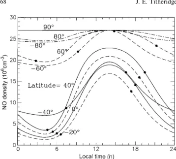
Fig. 3. Model values for the density at the peak of the NO layer, for June solstice conditions at F10.7"120 and Ap"10. Solid dots mark the times of sunrise and sunset
0600 to 1400 the NO density increases by a factor of 7. This is a compromise between the experimental results of Rusch et al. (1991), which suggest a factor of 10, and their theoretical model, which gives a factor of 6. At sunset the NO density is 25% less than the diurnal maximum (for latitudes up to $40°, as in Fig. 3). The night-time vari-ation, from 1900 to 0300, gives a near-exponential decay with a time-constant of about 5 h.
At latitudes above 60° the diurnal variation is reduced in accordance with the results referenced in Sect. 3.4. For a latitude of 90° the density at the peak of the NO layer is assumed constant at the value DH (Eq. 4). The diurnal variation is increased linearly at decreasing latitudes, giv-ing a change at 60° that is one-third of the variation at low latitudes. Thus for/ in the range 60°—90° we use
Dp"DH(//90#»(1!//90)). (9) For latitudes in the range/M to 60°, results are obtained by linear interpolation between the densities at these end points. A simple FORTRAN routine that carries out these calculations can be obtained from the author (email to [email protected]).
Diurnal variations in NO densities, calculated as above, are shown in Fig. 3. These curves are for June solstice conditions, with F10.7"120, at latitudes from 80°N to 80°S in steps of 20° and at the poles. With the globally symmetrical model, results apply equally well to the seasonal changes at a given site (apart from a small effect due to the last term in Eq. 7b). Thus the three solid-line curves labelled 40°, 0° and !40° also show the changes at a latitude of 40°N for summer, equinox and winter. Sunrise and sunset times at the different latitudes (or different seasons) are marked by solid dots in Fig. 3. These results should provide a reasonable first-order representation of likely changes in NO densities, at heights near 110 km, until more detailed observations are available.
3.6 Changes with height
The height variation of the NO density will be approxi-mated by ana-Chapman layer. This has a slightly sharper peak than theb-Chapman layer, agreeing better with most published curves, and gives
D(h)"Dp expM0.5(1!z!exp[!z])N, (10) where Dp"D0», and z"(h!hp)/HNO; hp is the height of the peak density of NO, and HNO is the assumed scale height (about 0.7 times that for a b-Chapman layer of similar thickness).
Vertical profiles tabulated by Barth (1990) show the peak density occurring at a mean height of 110 km. Ge´r-ard and Noe¨l (1986) give AE-D data for December, solar minimum, as a function of height and latitude. This shows
hp increasing from about 106 km at 30°N to 110 km at
40°S. This corresponds to hp"108#0.06(s·/), where (s ·/) gives the latitude in degrees, positive in summer, as in Eq. 2. Data from the SME satellite are shown as a function of height and of latitude by Ge´rard et al. (1990). Values of hp from these data show a change from about 110 km at !45° to 112 km at #45°, in June. There is no overall increase with solar flux, from F10.7"79 to 172, suggesting a variation hp"111#0.02(s·/).Ge´rard et al. (1990) also give model results for the daytime NO density as a function of height and latitude, for June solstice conditions at F10.7"80 and 200. These densities are dependent on assumed values for several constants, in particular the eddy diffusion coefficients (Fesen et al., 1990), which could change the peak heights. The model results show hp increasing in the summer hemisphere, and an increase with F10.7 which can be represented approximately by hp"109#0.01· F10.7# 0.05(s ·/). Model calculations by Ge´rard et al. (1993) give
hp"111 km, for values of F10.7 from 70 to 240.As a compromise between these results we will use the
expression
hp"110#0.005F10.7#0.04(s· /) km. (11) This gives a winter to summer variation of 2—3 km at mid-latitudes, and an increase of 1 km at solar maximum. Calculations and data from the AE-C satellite (Rusch
et al., 1991) show a significant diurnal variation of hp, with
an increase of 10—20 km for a few hours after sunrise, but the data are available only at heights above 135 km so the peaks are not fully defined.
Data from the AE-D satellite (Ge´rard and Noe¨l, 1986) show height variations corresponding to a scale height
HNO+5—8 km near solar minimum. Contour plots of
SME data (Ge´rard et al., 1990) give vertical scale heights of 7.5 and 8 km at F10.7"79 and 172. Corresponding model results have HNO+10 at F10.7"80, and 11.8 km at F10.7"200. Profiles calculated by Siskind and Rusch (1992) correspond to a scale height of 6—7 km at
F10.7+260. Smith et al. (1993) show an average of the
mean profiles tabulated by Barth (1990) for different con-ditions, including solar minimum and maximum; this pro-file corresponds to HNO+8 km. Solar minimum data
from the AE-C satellite, and corresponding model calcu-lations (Rusch et al., 1991), both indicate HNO+9 km. Ge´rard et al. (1993) also give model results which indicate
HNO+9 km, with no clear variation with solar flux. From
these data it seems reasonable to use a scale height increas-ing from about 8 to 9 km over the solar cycle, given by
HNO"8#0.005F10.7 km. (12) 4 Calculated profiles
4.1 Ion composition
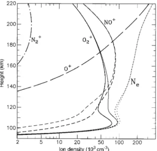
Ion composition results for typical summer day condi-tions are shown in Fig. 4. These are calculated using the EUVAC radiations and current values for the photo-ionisation cross-sections, as described in Sect. 2, with a full allowance for secondary ionisation. N`
2 is the main ion produced at heights of 110—190 km, but this converts rapidly to NO` (with about 10% to O` and O`
2) at heights below 170 km. Direct production of NO` from NO is very small, for zenith angles less than 80°, but indirect production causes NO` to be the major ion from about 125—180 km. Ignoring the effect of NO in the atmo-sphere gives ion densities shown by the fine lines in Fig. 4, with NO` predominating only down to 140 km. Under these conditions the loss of O`
2 by conversion to NO` is appreciably reduced at heights below 150 km. Since the recombination coefficient for O`2 is only half as large as for NO`, this gives a reduced overall loss rate and an increase of 9% in NmE.Figure 4 highlights a continuing problem in current models of the E region. Ion composition measurements from rockets indicate that NO` is the major ion near the peak of the E-layer (Keneshea et al., 1970; Danilov and Semenov, 1978; Swider and Keneshea, 1993). Most model-ling calculations show that NO` becomes less important than O`
2 at heights below 130—140 km, as discussed by Buonsanto et al. (1995). Results from the present model, with the improvements described in Sect. 2, do slightly better — giving a transition from NO` to O`
2 at a height near 120 km, for medium levels of solar activity (as in Fig. 4 and Table 1b).
The rocket results of Keneshea et al. (1970) and Swider and Keneshea (1993) show the ratio NO`/O`
2 reaching a maximum at heights of 105—125 km, where the propor-tion of NO` reaches 94—98%. These data are, however, for conditions near sunrise and sunset, with zenith angles of 89°—102° and F10.7"140. Model calculations for these conditions, using the normal 37 radiation bands (from 50—1050 As ), give NO`(90% of Ne at all heights. The present work adds the strong Lya line at 1216 As, as described in Sect. 2. For twilight conditions, this radiation is absorbed in the E region giving a large production of NO` by direct ionisation of NO (as described by Swider and Keneshea). For zenith angles of 90° and 95°, at
F10.7"140, the model calculations (shown in Table 1b)
give a peak NO` proportion of about 96%, at a height of 110—130 km, in reasonable agreement with the above rocket data.
Fig. 4. Ion densities for summer conditions at 40°N, withs"60° and F10.7"100. Fine lines show the results obtained if NO densities are reduced to zero
Mitra and Benerjee (1971) have also studied ion com-position variations, using rocket data from six mid-lati-tude flights ats"50°—60°. Three flights were at low solar activity, with a mean value F10.7"73, while three flights were at high activity with a mean F10.7"235. Both sets had a mean zenith angles"57°. The mean percentage of NO` ions obtained from these data are shown in italics in Table 1a and c. Bracketed values in Table 1b are obtained by linear interpolation in F10.7. Agreement with the pre-sent model results is good at all levels of solar activity, and all available heights (from 120 to 200 km). At F10.7"70 and 140 the agreement is excellent at all heights from 160 km down to (and including) 120 km.
The most complete data on observed ion composition in the E region is given by Danilov and Semenov (1978), based on 43 rocket mass spectrometer measurements carried out at latitudes of 30°—50°N. These data were combined and smoothed to produce tables giving the proportions of O`, O`
2 and NO` ions at heights of 100 to 200 km, for summer, equinox and winter conditions, at seven zenith angles (from 20° to 90°) and two levels of solar activity (F10.7"70 and 140). Expressions fitted to these data are used for ion-composition calculations in the International Reference Ionosphere (Bilitza, 1990). The tabulated results for NO` ions, for equinox conditions at four zenith angles, are reproduced in Table 1 and com-pared with the present model calculations. For heights above 130 km the agreement is quite good, with the Model and Rocket results differing by less than a factor of 1.2 in most cases. Differences are larger and more variable near 200 km, because of changes in the rate of O` increase at the base of the F-layer.
The present NO model is best defined for equinox conditions, at low and mid-latitudes (from Fig. 1a). At
F10.7"140, when the NO density is fairly large, the
Model and Rocket results in Table 1b are in reasonable accord at heights down to 120 km. Agreement is also quite
Table 1. The percentage of NO` ions at heights from 100 to 200 km, from the present Model calculations at a latitude of 40°N, and from mean Rocket results tabulated by Danilov and Semenov (1978). Values in italics are from rocket data analysed by Mitra and Benerjee (1971)
Height 100 110 120 130 140 150 160 180 200 km (a) F10.7"70 s"40° Model 7 23 35 45 50 51 48 33 13 % Rocket 36 49 55 56 56 53 49 37 17 57° Rocket — — 37 41 46 49 48 25 12 s"60° Model 9 22 37 43 49 51 49 34 13 Rocket 47 54 58 56 56 53 49 37 17 s"80° Model 46 23 39 47 48 51 54 39 15 Rocket 66 66 65 63 58 54 52 40 22 s"90° Model 53 81 50 50 58 66 67 58 17 Rocket 91 81 76 74 66 63 63 54 34 (b) F10.7"140 s"40° Model 13 33 46 53 55 53 49 32 12 % Rocket 36 49 55 56 56 53 45 27 10 (57° Rocket — — 53 52 53 53 51 30 15' s"60° Model 20 34 52 55 57 55 52 34 13 Rocket 46 54 57 56 56 53 45 27 10 s"80° Model 78 46 58 61 61 61 61 45 18 Rocket 66 66 65 63 58 54 48 33 14 s"90° Model 81 95 73 67 71 75 77 70 32 Rocket 91 81 76 74 66 73 58 46 28 s"95° Model 74 89 96 97 96 91 89 88 51 (c) F10.7"235 57° Rocket — — 77 67 62 59 56 39 20 s"60° Model 24 36 58 62 63 62 57 38 19 %
good (at all heights) near sunrise and sunset, when Lya radiation gives a large production of NO` in the E region. At heights of 100—110 km, however, model results for the proportion of NO` ions are commonly about half of that indicated by the rocket data at zenith angles up to 80°. The differences are largest at F10.7"70, due to the almost complete absence of any solar cycle change in the ‘Rocket’ results. This seems unrealistic, in view of the clear changes in NO density (Fig. 1a), and in the independent rocket data at s"57° in Table 1. Thus the Rocket data at
F10.7"70 may give NO` ratios which are up to 50% too
high at 120 km, fors"60°.
For F10.7"140, and s480°, the comparison in Table 1b suggests that the model results are acceptable at heights down to about 120 km. At lower heights the cal-culated proportion of NO` is less than the rocket results by a factor of 1.5 at 110 km, and a factor of about 2 at 100 km. The difference is caused by a rapid decrease in calculated NO` densities, at heights below about 115 km, and the large increase in O`
2 production at the E-region peak near 108 km. N`
2 ionisation produced at these heights is converted almost entirely to NO`, with a rate constant about 1000 times greater than for the conversion of O`2 to NO`. With our current understanding of E-region chemistry, this leaves four possibilities for increas-ing the proportion of NO` ions in the E region:
(1) Increase the NO density at low heights, to increase the conversion of O`
2 to NO. Approximate agreement with the Rocket data of Table 1, at a height of 110 km and
s(80°, is obtained if NO densities are increased by a factor of about 2 at F10.7"140 (and a factor of 3 at
F10.7"70). These changes reduce the calculated values of NmE by about 7%.(2) Increase the rate constants for the conversion of
O`
2 to NO`. This has basically the same effect as (1). Reaction rates must be increased by a factor of 2—3, giving a decrease of about 7% in calculated values of NmE. Other reactions that produce NO` are negligible at 110 km, because of the low densities of O` and N`.
(3) Increase the direct production of NO` near 110 km. The peak absorption of Lya can be raised to this height by increasing the ionisation cross-section for NO. The change required is a factor of several hundred, and gives an increase of about 20% in NmE.(4) Decrease the loss rate for NO`. Loss occurs only through direct recombination, with a rate constant just over twice that for the direct recombination of O`2. De-creasing this rate by a factor of 2 gives adequate NO` at 110 km, for F10.7"140. It also gives too high a propor-tion of NO` (about 70%) at heights near 150 km, and an unacceptable increase of 35% in NmE.Errors of 100% or more in the different rate constants seem unlikely, and the data in Fig. 1a appear to rule out a similar increase in equinoctial NO densities. Errors of 100% in the rocket measurements of NO`, at low heights, also seem unlikely — although the disparity between the independent rocket results at s"57° and s"60° in Table 1 suggests that further experimental data are
necessary. Perhaps the solution of this problem will involve several small adjustments. These could produce changes of the order of 5% in calculated values of
NmE, and in the width and depth of the E-F1 valley
region.
4.2 Electron density
Calculated summer day profiles are compared with the experimentally based IRI-90 value of NmE in Fig. 5. When secondary ionisation is omitted we get the results shown by the left-most broken line, with a peak (E-layer) density 30% less than the IRI value for these conditions. The continuous line, including a full allowance for photo-electrons and ionising radiations down to 25 As (as de-scribed in Titheridge, 1996), gives much better agreement. The EUVAC radiation model uses the F74113 reference spectrum with fluxes increased by a factor of 2 from 150—250 As , and by a factor of 3 at wavelengths j(150 As, to improve agreement with measured photoelectron fluxes (Richards et al., 1994). If this latter factor is increased to 4.0, giving an additional 33% increase in the fluxes at j(150 As, we get the profile shown by the heavy broken line in Fig. 5. This is now only 3% below the IRI value for these summer conditions. Increasing the EUV fluxes by 18% at all wavelengths gives a similar result, as shown by the fine broken line.
With no adjustment to the EUVAC radiations, agree-ment with the IRI value of NmE can be obtained by ignoring the presence of neutral NO; this gives the profile shown by the dotted line in Fig. 5. This approach does not seem acceptable, however, since the presence of substan-tial amounts of NO seems well-established. Agreement can also be obtained if the production of secondary ionisation is increased by about 60%. This can just be achieved by reducing the electron excitation cross-sec-tions for O2 and N2 by a factor of 4 or more (Titheridge, 1996), but this also conflicts with current measurements. Figure 6 shows the changes that can be obtained by altering the radiation models and ionisation constants. The heavy continuous line is the present result, as in Fig. 5. Changing to the earlier photoionisation cross-sec-tions of Richards and Torr (1988) gives the result shown by the thin continuous line. This agrees reasonably well with the value of NmE from the IRI standard. The in-creased ionisation near 107 km is, however, obtained at the expense of a large decrease at greater heights, giving an E-F valley that is wider (27 km) and deeper (22%) than normally expected. The thick chain line uses the modified Hinteregger radiations (with the same radiation bands, as described in Sect. 2, and fluxes doubled atj(250 As as in Richards and Torr, 1988). This gives densities matching the IRI value of NmE very closely, but again the E-F valley is rather too large. Use of Hinteregger radiations with the older cross-sections gives a large increase in NmE and far too large a valley region, as shown by the fine chain line in Fig. 6. Thus acceptable values for both the peak density in the E region, and the valley between the E and F1 regions, are most readily obtained by using the EUVAC radiation model (preferably with a 33% increase atj(150 As), in
Fig. 5. E-region profiles calculated for summer conditions at 40°N, withs"60° and F10.7"120. All curves use the EUVAC radiation model of Richards et al. (1994), and current values for the ionisation cross-sections (from Fennelly and Torr, 1992)
Fig. 6. E-region profiles calculated for summer noon conditions, as in Fig. 5. Continuous lines use the EUVAC radiation model, with ‘normal’ (heavy line) or reduced ( fine line) ionisation cross-sections.
Chain lines give corresponding results for the modified Hinteregger
radiations of Richards and Torr (1984, 1988)
conjunction with recent values for the photoionisation cross-sections.
Comparisons between model results and observed elec-tron densities in the E region have also been made by Buonsanto (1990) and Buonsanto et al. (1992, 1995). These use data obtained with the Millstone Hill radar, and so relate to individual occasions rather than the mean
ionosphere used in the present work. In the most recent study (Buonsanto et al., 1995) plotted results show that use of the older ionisation cross-sections, instead of the more recent values from Fennelly and Torr (1992), gives an increase of about 8% in NmE. This compares well with the increase of 9% in Fig. 6. There is also a similar increase in valley width, from 17 to 27 km in Fig. 6 and from 18 to 30 km in Fig. 2 of Buonsanto et al. (1995) (using EUV fluxes from rocket data).
Figures 3 to 6 of Buonsanto et al. (1995) show the effect of changing from the EUVAC radiation model to, among others, the modified Hinteregger model. This gave in-creases in NmE of 10%, 20%, 23% and 29% under differ-ent conditions. The mean change is much larger than the increase of 12% found in Fig. 6 of the present work. Buonsanto et al. note, however, that their ionospheric model gives insufficient secondary ionisation with the EUVAC radiations. This is because it uses fixed ratios of secondary- (Pe) to-primary (Pi) ionisation, as a function of optical depth, based on the calculations of Richards and Torr (1988) using the earlier flux model. The EUVAC model has larger fluxes in all bands that produce second-ary ionisation, and less in other bands. This gives a signifi-cant increase in Pe/Pi, that is obtained automatically from the approach used in the present work (Sect. 2). Thus the smaller increase found here, on changing from EUVAC to the Hinteregger radiations, is due to the higher secondary production obtained with the EUVAC spectrum. Reduc-ing this secondary production by 35% gives about the same mean Pe/Pi ratio as for the Hinteregger radiations, and a decrease of 8% in NmE. Changing from this result to one using the Hinteregger radiations then gives an in-crease of 21% in NmE, in full agreement with the mean increase found by Buonsanto et al. (1995).
Other ionospheric data provide support for higher fluxes in the short radiation bands, as in the EUVAC model. Only wavelengths less than 150 As , or longer than 1000 As , produce significant amounts of ionisation at heights near 110 km. Calculations show that, for the EU-VAC model, short wavelengths produce 62% of the ionisation at F10.7"60, 66% at F10.7"100 and 69% at
F10.7"200. These figures agree well with the results of
eclipse measurements by Bomke et al. (1970), who found that 68% of the ionisation was from the short-wavelength region. For the modified Hinteregger radiations, short wavelengths produce only about 45% of the total E-re-gion ionisation, for all values of F10.7. This is significantly less than the experimental result, and suggests that the factor-of-2 increase used atj(250 As, in the ‘modified’ model, is insufficient.
5 Changes with solar flux
In both the EUVAC and Hinteregger radiation models, the EUV fluxes are a function of the daily F10.7 index and the average value (F10.7A) over an interval of 81 days centred on the current date. All calculations in this paper take F10.7A"F10.7, so that results apply to long-term variations in solar flux. The two parameters (F10.7 and F10.7A) are given equal weights in the EUVAC model.
Day-to-day fluctuations in solar activity, about a constant mean level, will then produce changes in EUV that are just half as large as for long-term variations.
In both radiation models the intensities of all radi-ations increase linearly with the 10.7-cm flux, since they are obtained by linear interpolation between data sets at
F10.7"80 and 200 (Richards et al., 1994). Between these
sets, the intensities of different bands increase by factors of 1.4 to 4. Taking only those radiations that ionise below 135 km, and weighting each band by the amount of ionisation it produces, gives a mean increase by a factor of 1.88. Thus for the EUVAC radiations, at E-region heights, the ionisation production rate Q varies as F10.7#56. Normal E-region theory assumes quadratic recombina-tion, giving dN/dt"Q!aN2 where a is the recombina-tion coefficient. Time-constants near the E peak are only about 2 min, so that densities are always close to the equilibrium value. The density at the peak of the E-layer is then proportional to the square root of the production rate, giving
NmE"A(F10.7#B)0.5, (12)
where A is some constant, and B"56 for the EUVAC radiation model and simple quadratic recombination.
Model calculations for noon equinox conditions, using a fixed atmospheric temperature and composition with no NO, give a variation of NmE with F10.7 that corresponds to B"53 in Eq. 12. Thus densities increase slightly faster than predicted by simple theory, indicating that a small part of the recombination follows a linear (rather than quadratic) form. Including a fixed amount of NO (corre-sponding to F10.7"100, at noon) gives a slightly in-creased loss rate for O2`, through the charge-exchange reaction O`
2#
NOPO2#NO`. This is followed by re-combination of NO`, with a rate coefficient about twice that for the direct recombination of O`
2. The first (charge exchange) step of this process introduces some depend-ence on linear loss processes. Calculated values of NmE then vary more rapidly with F10.7, giving B"45 in Eq. 12.
Calculations with no NO, but allowing the atmosphere to vary with F10.7 (as given by the MSIS model, for equinox conditions) give B"60 in Eq. 12. Thus normal composition changes, as given by the MSIS86 atmo-spheric model, slightly reduce the variation of NmE with solar activity. When a varying NO is also included we get
B"95, since the increased NO densities near solar
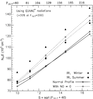
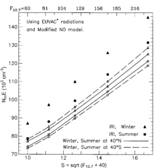
max-imum give larger loss rates and a larger reduction in NmE. Figure 7 shows the calculated variation of NmE with solar flux, for summer noon conditions at a latitude of 40°N. With a solar zenith angle of 16.5°, changes under these conditions will reflect most directly the changes in the ionising radiation. Results are plotted against (F10.7 #40)0.5, since this gives an almost linear variation for most data sets and is accurately linear for the experi-mentally based IRI values. The continuous line in Fig. 7 is from the full atmospheric model, giving a variation corre-sponding to B"110 in Eq. 12. When NO is neglected (dotted line) the model values correspond to B"68 — still slightly greater than the value of 56 expected for simple
Fig. 7. The electron density at the peak of the E-layer (NmE) plotted as a function of (F10.7#40)0.5, where F10.7 is the 10.7-cm solar flux (top scale). All results are for summer noon conditions at a latitude of 40°N, withs"16.5°. Solid dots represent mean observed values for these conditions, from the IRI-90 empirical model. The
continu-ous line is from calculations using the EUVAC radiation model. Broken and dotted lines are obtained when the changes of NO
density with F10.7 are suppressed. Points marked#are with half the normal NO
quadratic recombination. The results plotted as#in Fig. 7 are obtained when the NO densities are halved. These points fall roughly halfway between the solid and dotted lines, showing that the variation of NmE with NO density is approximately linear.
The fastest change of NmE with F10.7 is obtained by removing the increase of NO near solar maximum, and giving increased emphasis to linear recombination pro-cesses. These requirements are both met by using a fixed NO density. Results when the NO density is held constant at the value corresponding to F10.7"120 are shown by the broken line in Fig. 7. This has a slope corresponding to B"49 in Eq. 12. Use of fixed NO densities correspond-ing to F10.7"180 gives B"46, but this requires an unacceptably large NO density at solar minimum and gives too-small values of NmE at all times.Our best current estimate of mean observed values of
NmE, under different conditions, comes from the IRI-90
ionospheric model (Bilitza, 1990). The expressions for
NmE in this model are derived from an analysis of a large
experimental data base, by Kouris and Muggleton (1973a, b), and provide a good representation of mean observed values as a function of solar zenith angle, lati-tude, season and solar flux. The solid dots in Fig. 7 show the values of NmE given by the IRI-90 model for summer noon conditions at 40°N, with s"16.5°. The plotted values are for F10.7"60, 85, 120, 170 and 240. At solar minimum these points are only 5% above the full model results (solid line). At F10.7"170, however, the IRI values are 16% above the full model. The slope of the IRI
variation corresponds to B"40.4 in Eq. 12, showing an appreciably faster change than in any model results using the EUVAC radiations.
The change of NmE with F10.7, as given by the IRI-90 model, is larger than that which would be obtained from the EUVAC radiation model assuming that all loss is quadratic (giving B"56). Even with an artificially large and constant value for the assumed density of NO, calcu-lations using the EUVAC model give B"46. This corre-sponds to a solar-cycle increase that is significantly below the experimental value. Other possible changes in the production or loss mechanisms near solar maximum seem little help. Increased electron temperatures could reduce the recombination rates for O`
2, N`2 and NO`, but an increase of 100% in ¹e!¹n gives an increase of only 3.5% in NmE. Alternatively the direct production of O`2 could be increased by a larger proportion of O2 in the atmosphere, near solar maximum. Increasing the O2 dens-ities by 40%, and decreasing N2 by 10% to keep the same overall density, gives an increase of 6% in NmE. This is barely sufficient to explain the changes at solar maximum, and composition errors of this size in the MSIS86 model (at solar maximum only) seem unlikely. Buonsanto (1990) has shown that an overall decrease in neutral densities will give increased electron densities. For a 25% decrease in the density of all components, the present calculations give an increase in NmE which varies from 2% at solar minimum to 4% at solar maximum. These changes, at a height of 110 km, are appreciably less than the changes of 5—10% found by Buonsanto at 180 km, and are not sufficient to explain the too-small values of NmE near solar maximum.
Some changes in E-region chemistry near solar max-imum cannot be ruled out. As noted in Sect. 4.1, current modelling calculations give ratios NO`/O`2 which appear significantly less than some experimental data in the lower E region. This suggests that our knowledge of E-region chemistry is incomplete. Introduction of new reactions, or new temperature variations, could result in an increased solar-cycle variation in calculated values of NmE.A more likely way to provide increased ionisation near solar maximum is through revision of the EUV model. An increase of 20% in the solar maximum reference spectrum used in the EUVAC model (at F10.7"200) gives results shown by the broken line in Fig. 8. This matches the slope of the IRI variation quite accurately, giving B"39 in Eq. 12. These results include the full NO allowance, and give values of NmE which are about 6% below the IRI values throughout the solar cycle.
The chain line in Fig. 8 shows the variation calculated using the modified Hinteregger radiations (Richards and Torr, 1988). These results match the IRI values quite closely, at all stages of the solar cycle, with an error that decreases from !3% at F10.7"60, to 0% at F10.7"230. Thus the solar-cycle increase used in the Hinteregger model slightly exceeds that required to match the ob-served changes in NmE. This occurs because the H-Lyb radiation, that provides most O`
2 ionisation in the E re-gion, has a solar cycle increase that is 27% larger in the Hinteregger data than in the EUVAC model. The Hin-teregger spectrum does, however, give E-F region valleys
Fig. 8. Changes in NmE obtained with different radiation models, using the full atmospheric model (with varying NO). The EUVAC model with a 20% increase in fluxes at high solar activity gives the
broken line. The chain line gives results obtained using the modified
Hinteregger radiations
which are appreciably too large throughout the solar cycle (as in Fig. 6). Thus optimum agreement with observations requires a spectrum similar to that used in the EUVAC model, with fluxes increased near solar maximum to match the changes given by the Hinteregger data.
The IRI-90 model corresponds to the CCIR78 model, based on the E-region studies of Kouris and Muggleton (1973a, b). For CCIR use this was later replaced by the simpler CCIR86 model, which ignores seasonal or latitude changes and assumes that ionospheric production varies as F10.7. Thus the CCIR86 model uses Eq. 12 with B"0. Values of NmE calculated from this model are shown as squares in Fig. 8. While they agree with the IRI values at
F10.7+108, the solar variation is much too large. The
CCIR86 model could be greatly improved by substituting 0.73(F10.7#40) for F10.7.
6 Seasonal changes
Early studies of the E region revealed a seasonal anomaly at mid-latitudes, with NmE 5—15% higher in winter than in summer (Appleton, 1963; Muggleton, 1972). A detailed analysis by Kouris and Muggleton (1973a, b) used monthly median data from 45 stations, averaged over a full sunspot cycle. Data were corrected for changes in the solar zenith angle, and in the sun-earth distance. Results showed mean values of NmE that were approximately constant at the equator and in winter, but decreased by about 7% in summer. This change is incorporated in the IRI-90 model, as shown by the solid circles (summer) and triangles (winter) in Fig. 9.
Relative to the summer values of NmE, the IRI model gives an increase in winter of about 2%, 10% and 12% at
Fig. 9. The variation of NmE with solar flux for summer (circles) and winter (triangles). Results are for a latitude of 40°N, at a constant solar zenith angles"65°. Solid symbols are from the IRI empirical model. Continuous and dotted lines are from model calculations with and without the inclusion of NO
latitudes of 20°, 40° and 60°, respectively. The IRI data plotted in Fig. 9, for a latitude of 40°N, show a constant increase of 10.4% from summer to winter. When the presence of NO is ignored, model calculations give the dotted lines that show a decrease of 1.0% (solar minimum) to 2.4% (solar maximum) in winter. This is caused by composition changes in the MSIS86 atmospheric model. In the southern hemisphere, these changes give an increase in winter, of 2.9% (solar minimum) to 3.6% (solar max-imum). Thus the changes in the MSISI86 atmospheric model are basically annual. They are larger and in the right direction to produce the observed seasonal anomaly in NmE in the southern hemisphere, but are too small by a factor of about 3.
At solar minimum, in both hemispheres, inclusion of NO decreases the summer values of NmE by about 6%. In winter the change is only 1%, since the NO density is only about one-quarter of the summer value (Fig. 1b). As a re-sult, the presence of NO gives a small seasonal anomaly in the northern hemisphere, with NmE increasing by about 4% from summer to winter (at a fixed zenith angle). In the southern hemisphere, the annual composition changes in the MSIS86 model combine with the NO variations to produce a seasonal anomaly of about 8%, which is close to the observed value.
Near solar maximum, the inclusion of NO gives a re-duction of 11% in the summer values of NmE, as shown in Fig. 9. In winter the decrease in NmE is 9%, only slightly less than in summer. This is because the satellite data used for the present model give approximately the same abso-lute change in NO from winter to summer at all levels of solar activity (Fig. 1b). Thus the summer increase in NO is too small to explain the seasonal anomaly in NmE near solar maximum.
The seasonal anomaly is observed in both hemispheres, so it cannot be caused by changes in the solar radiation. Changes in atmospheric composition or temperature also seem inadequate to explain the observations, as discussed above. This leaves movements as a possible cause. Electric fields, or winds in the neutral atmosphere, can cause a vertical drift of ionisation at mid-latitudes. If the drift velocity U changes with height, we get an additional production term dQ"div(N · U) in the continuity equa-tion. At the height of the peak this reduces to
dQ"N · dU/dh. Assuming a quadratic loss process in the
E-layer, the normal relation Q"aN2 then gives the change in peak density, due to the vertical drift, as
dN"(1/2a) dU/dh. (13)
The rate coefficienta, for direct recombination of O` 2, is about 1.5]10~7 cm3 s~1. If the vertical drift U changes by 10 m s~1 in a vertical distance of 10 km, we get
dN"3000 cm~3 from Eq. 13. For a typical daytime
E-layer with NmE+1· 105 cm~3, this is a change of 3% in
NmE. Allowing for the fact that over 30% of the daytime
recombination is via additional loss processes (such as charge exchange with N or NO, to give NO`), reduces the expected change in NmE to less than 2%. This is con-firmed by full model calculations. A vertical drift that changes by 10 m s~1 in 10 km alters NmE by 1.8% when the presence of NO is ignored, and by 1.6% when it is included. The percentage change is somewhat larger near sunrise and sunset since, as shown by Eq. 13, the absolute change dN is independent of N.
At mid-latitudes, the above vertical drifts correspond to a horizontal (meridional) wind that changes by least 20 m s~1 between heights of 100 and 110 km. Normal ionospheric winds (reviewed in Titheridge, 1995) show a height variation of about half this amount, in a direction that would decrease NmE by up to 1% near noon. To obtain a 10% difference between summer and winter would require a regular seasonal change in the wind shear through about ten times the mean value. There is no variation of this type in current models or observations. Since the wind shears cannot be maintained over a large height range, any such effect would be accompanied by large seasonal changes in the size of the E-F1 valley region, which have not been observed.
Vertical movements of ionisation can also be caused by horizontal electric fields, and fields associated with the equatorial electrojet have been postulated as a cause of the seasonal anomaly in NmE (Kouris and Muggleton, 1973b). This was based partly on the result that, for a simple Chapman layer, a steady vertical drift will pro-duce some change in NmE. No numerical results were given, but the simplified equation shown gives a change of about 10% in NmE for a vertical drift U"30 m s~1. Full model calculations show a change of only 1.1% in NmE for a steady drift of this size, and unrealistically large drifts are required to obtain a 10% change in NmE. This leaves the question as to whether electric fields can produce a large vertical drift gradient in the E region. The results of Richmond et al. (1980) show vertical drifts at mid-latit-udes of 5—30 m s~1, at F-region heights, with day-to-day
variations of around 100%. These drifts apply to an entire field line, so there can be no large seasonal changes. Latitude variations also seem inadequate to give a consis-tent change of 10 m s~1 in a vertical distance of only 10 km, in the E region. Thus in the absence of full quanti-tative calculations, it appears unlikely that electrojet fields could give sufficiently large, regular variations in the verti-cal drifts to account for the E-region seasonal anomaly.
These difficulties make it appropriate to re-examine the possibility of obtaining a larger seasonal variation from changes in the NO density. The mean summer and winter curves of Fig. 1b, obtained as fits to the plotted data, are rather unsatisfactory from a physical viewpoint. As the solar radiation increases, we would expect a similar in-crease in the mean NO densities in both winter and summer. Production is from direct or indirect dissociation of N2, and this gas has no large seasonal or solar-cycle changes in the E region. The loss processes depend prim-arily on neutral N(4S), which also has little seasonal or solar variation in the MSIS86 model (although these data may be unreliable in the E region, as noted in Sect. 3.1). Theb-type loss should give NO densities that vary in the same way as the solar radiation. This is confirmed in calculations by Fuller-Rowell (1993), who used a one-dimensional, globally averaged model of the thermo-sphere to determine the changes with solar activity. Results showed a change in NO densities by a factor of 4, for F10.7 increasing from 70 to 190. This agrees accurately with the change in Fig. 1a, defined by mean SME measurements over the equator.
At F10.7"70, Fig. 1b gives an increase by a factor of 2.3 from winter to summer. This seems about right. Multi-plying the value of coss at noon by the number of hours from sunrise to sunset, to give a rough measure of the total solar input, gives a summer-to-winter ratio of 2.3 at a lati-tude of 30°. At F10.7"190, however, the curves in Fig. 1b give a summer increase by a factor of only 1.24. This change seems far too small, unless there are large seasonal changes in atmospheric composition, that vary with solar activity. NO time-constants are too short to allow hori-zontal mixing between hemispheres, so we would expect the summer/winter ratio to be roughly constant through-out the solar cycle.
To obtain a more nearly constant ratio, Eq. 2 can be modified to
D0"A#B(F10.7!100)
!
0.0008(F10.7!100)2]106 cm~3. (14) where A"14.8#0.1s ·/#C, B"0.22#0.026C and
C is a correction term given by C"0.05s ·/. Setting C"0.0 gives the original form of Eq. 2. For latitudes of
30°N and 30°S, in summer and winter, Eq. 14 gives the curves shown as dotted lines in Fig. 1b. The seasonal change in NO density, at a latitude of 30°, is now a factor of 2.2 at F10.7"80 and a factor of 1.8 at F10.7"180. The dotted lines in Fig. 1b provide a rather poor fit to the SME data at F10.7'120, particularly in winter, but this must be accepted if we wish to avoid a greatly reduced seasonal change near solar maximum. The maximum fit error of about 20% may still be acceptable, since there are