HAL Id: hal-01983169
https://hal.archives-ouvertes.fr/hal-01983169
Submitted on 24 Apr 2019
HAL is a multi-disciplinary open access
archive for the deposit and dissemination of
sci-entific research documents, whether they are
pub-lished or not. The documents may come from
teaching and research institutions in France or
abroad, or from public or private research centers.
L’archive ouverte pluridisciplinaire HAL, est
destinée au dépôt et à la diffusion de documents
scientifiques de niveau recherche, publiés ou non,
émanant des établissements d’enseignement et de
recherche français ou étrangers, des laboratoires
publics ou privés.
67P/Churyumov-Gerasimenko with Rosetta trajectory,
rotation, and water production measurements
Nicholas Attree, Laurent Jorda, Olivier Groussin, Stefano Mottola, Nick
Thomas, Yann Brouet, Ekkehard Kührt, Martin Knapmeyer, Frank Preusker,
Frank Scholten, et al.
To cite this version:
Nicholas Attree, Laurent Jorda, Olivier Groussin, Stefano Mottola, Nick Thomas, et al.. Constraining
models of activity on comet 67P/Churyumov-Gerasimenko with Rosetta trajectory, rotation, and
water production measurements. Astronomy and Astrophysics - A&A, EDP Sciences, In press.
�hal-01983169�
January 10, 2019
Constraining models of activity on comet
67P/Churyumov-Gerasimenko with Rosetta trajectory,
rotation, and water production measurements
N. Attree
1, 2, L. Jorda
1, O. Groussin
1, S. Mottola
4, N. Thomas
3, Y. Brouet
3, E. Kührt
4, M. Knapmeyer
4,
F. Preusker
4, F. Scholten
4, J. Knollenberg
4, S. Hviid
4, P. Hartogh
5, and R. Rodrigo
61 Aix Marseille Univ, CNRS, CNES, Laboratoire d’Astrophysique de Marseille, Marseille, France
2 Earth and Planetary Observation Centre, Faculty of Natural Sciences, University of Stirling, UK e-mail:
3 Physikalisches Institut, Universität Bern, Sidlerstrasse 5, 3012 Berne, Switzerland
4 Deutsches Zentrum für Luft-und Raumfahrt (DLR), Institut für Planetenforschung, Rutherfordstraße 2, 12489 Berlin,
Germany
5 Max-Planck-Institut für Sonnensystemforschung, Justus-von-Liebig-Weg 3, 37077 Göttingen, Germany
6 International Space Science Institute, Hallerstrasse 6, 3012 Bern, Switzerland
January 10, 2019
ABSTRACT
Aims.We use four observational data sets, mainly from the Rosetta mission, to constrain the activity pattern of the
nucleus of comet 67P/Churyumov-Gerasimenko.
Methods.We develop a numerical model that computes the production rate and non-gravitational acceleration of the
nucleus of comet 67P as a function of time, taking into account its complex shape with a shape model reconstructed from OSIRIS imagery. We use this model to fit three observational data sets: the trajectory data from flight dynamics; the rotation state, as reconstructed from OSIRIS imagery; and the water production measurements from ROSINA, of 67P. The two key parameters of our model, adjusted to fit the three data sets all together, are the activity pattern and the momentum transfer efficiency (i.e., the so-called “⌘ parameter” of the non-gravitational forces).
Results.We find an activity pattern able to successfully reproduce the three data sets simultaneously. The fitted activity
pattern exhibits two main features: a higher effective active fraction in two southern super-regions (⇠ 10 %) outside perihelion compared to the northern ones (< 4 %), and a drastic rise of the effective active fraction of the southern
regions (⇠ 25 35 %) around perihelion. We interpret the time-varying southern effective active fraction by cyclic
formation and removal of a dust mantle in these regions. Our analysis supports moderate values of the momentum
transfer coefficient ⌘ in the range 0.6 0.7; values ⌘ 0.5 or ⌘ 0.8degrade significantly the fit to the three data sets.
Our conclusions reinforce the idea that seasonal effects linked to the orientation of the spin axis play a key role in the formation and evolution of dust mantles, and in turn largely control the temporal variations of the gas flux.
Key words. comets: general, comets: individual (Churyumov-Gerasimenko), planets and satellites: dynamical evolution and stability
1. Introduction
The sublimation of ices when a comet is injected from its reservoir to the inner solar system triggers the emission of molecules. This outgassing produces in turn a reaction force which can accelerate the comet nucleus in the opposite direction. The perturbing effect of cometary activity on the trajectory of comets has been established in the 1950’s in the pioneering work by Whipple (1950). At that time, it was clear that most comet trajectories were affected by a significant nongravitational acceleration (hereafter “NGA”) linked to their activity around perihe-lion (Marsden 1968). Shortly after, a theoretical model describing the nongravitational force (hereafter “NGF”) produced by the sublimation of ices was established by Marsden et al. (1973). This model was based on a simple function describing the heliocentric dependence of the sublimation of water ice of a comet, combined with
constant scaling parameters A1, A2 and A3 describing the
amplitude of the NGA along the three components (radial, transverse, normal) in the orbital frame of the comet. The model has been modified by Yeomans & Chodas (1989) to incorporate an asymmetric term used to describe the shift of the maximum of activity with respect to perihelion. It is worth mentioning here that these simple models are still in use nowadays to fit astrometric measurements, and hence to describe cometary orbits.
More sophisticated models have been introduced since then. Images acquired during the flyby of comet 1P/Halley by Giotto showed narrow dust jets (Keller et al. 1987), leading to the idea that the activity may be confined to localised areas. This led to a new model of nongravitational acceleration (Sekanina 1993) in which the outgassing originates from discrete areas at the surface of a rotating nucleus. Szutowicz (2000) used Sekanina’s
model to fit astrometric measurements of comet 43P/Wolf-Harrington obtained during nine perihelion passages. She also compared the modelled production rate with visual lightcurves used as a proxy for the activity of the comet (Szutowicz 2000). Recently, Maquet et al. (2012) revisited Sekanina’s approach with a model in which the activity is parametrised by the surface fraction of exposed water ice in “latitudinal bands” at the surface of an ellipsoidal nucleus. More accurate ground-based measurements as well as space missions to comets offered the opportunity to incorporate new physical processes in models of the NGA. Rickman (1989) used the change of the orbital period of comet 1P/Halley caused by the NGA to extract its mass and density. The detailed description of the local outflow velocity incorporated a “local momentum transfer coeffi-cient” ⇣l, originally called ⌘ in the improved description
of the solid-gas interface introduced by Crifo (1987). This coefficient represents the fraction of the emitted gas’s momentum (dependent on its thermal velocity) which needs to be considered in the calculation of the momentum transfer, and thus of the NGF (see Crifo 1987). Davidsson & Gutiérrez (2004) used 2D thermal modelling including thermal inertia, self-shadowing, self-heating and an activity pattern to fit the NGA of comet 19P/Borrelly. They could retrieve the mass of the nucleus and constrain the direction of the spin axis. The method was also applied to comets 67P/Churyumov-Gerasimenko (Davidsson & Gutiérrez 2005), 81P/Wild 2 (Davidsson & Gutiérrez 2006), and 9P/Tempel 1 (Davidsson et al. 2007), all targets of space missions.
The exploration of comet 1P/Halley in 1986 also yielded the discovery of the non-principal axis rotation of this comet (Samarasinha & A’Hearn 1991). Since then, the torque of the NGF was thus identified as the major effect responsi-ble for changes of the rotational parameters (Samarasinha et al. 2004a, and references therein). Its modelling is re-quired to understand the observed change in the rotational parameters of cometary nuclei, as well as the apparition of non-principal axis rotations. Changes in the spin pe-riod of several comets have been detected from the anal-ysis of lightcurves (Mueller & Ferrin 1996; Gutiérrez et al. 2003; Samarasinha et al. 2004b; Drahus & Waniak 2006; Knight et al. 2011; Bodewits et al. 2018). Predictions of the expected change in the direction of the spin axis and spin period for comets 81P/Wild 2 (Gutiérrez & Davidsson 2007) and 67P/Churyumov-Gerasimenko (hereafter “67P”, Gutiérrez et al. 2005) have been made. Recently, a change in the spin period of comet 67P has been clearly identified between the 2009 and 2015 perihelion passages (Mottola et al. 2014) based on early images acquired by the OSIRIS camera aboard Rosetta. Keller et al. (2015) showed that the spin period variation curve of 67P is controlled at first order by the bilobate shape of the nucleus.
Thanks to its long journey accompanying comet 67P, Rosetta provides a unique chance to record measure-ments of most parameters involved in the modelling of the NGF. The mass of the comet has been retrieved by Pätzold et al. (2016) from the radio science experiment aboard the spacecraft. The shape has been retrieved from a stereophotogrammetric analysis of a subset of OSIRIS im-ages (Preusker et al. 2017), leading to an accurate knowl-edge of the moments of inertia. The activity pattern has been constrained in the early phase of the mission by
Marschall et al. (2016, 2017) from ROSINA measurements in the form of “effective active fractions” associated to ge-ological regions. The total water production rate has been constrained from ROSINA measurements, complemented by ground-based observations (Hansen et al. 2016). Finally, the spin period has been monitored throughout the mission by ESA’s flight dynamics and OSIRIS teams before (Jorda et al. 2016) and after (Kramer et al. 2019) perihelion. The latter (Kramer et al. 2019) modelled the temporal evolu-tion of the rotaevolu-tional parameters, comparing it with the measured change in spin period and spin axis orientation. The aim of this article is to try to reproduce three data sets derived by several Rosetta instruments (see section 2) with a model of the NGF (see section 3) in order to retrieve: (i) the local effective active fraction and its temporal vari-ations around perihelion, and (ii) a recommended value for the momentum transfer coefficient ⌘ (see section 4). The results will be discussed in section 5, together with recom-mendations for the calculation of NGF of other comets.
2. Observational constraints
In this section, we describe the observational data, mainly obtained by the Rosetta spacecraft, to which we will at-tempt to fit our NGF model.
2.1. Water production rate
The total water production rate is an important constraint for any model of cometary activity, and a significant ef-fort has been made to measure it for 67P. As summarised by Hansen et al. (2016), a number of different instruments have all been used and comparing and synthesising their results in non-trivial. Here, we use the ROSINA (Rosetta Orbiter Spectrometer for Ion and Neutral Analysis) mea-surements, empirically corrected for spacecraft position, as our observed data points, OQ. Hansen et al. (2016) describe
how estimating the uncertainty in these data, Q, is difficult
so we use the bounds on the power-law, fitted with helio-centric distance to the inbound ROSINA data, as given in their Table 2.
We point out that ROSINA data are inferred from lo-cal measurements in the coma of 67P. Around perihelion, the spacecraft was located at a distance of 200 km from the nucleus, making it difficult to infer a total production rate, whilst ground-based observations (see, for example, Bertaux 2015) have also suggested a variation in peak pro-duction between perihelion passages. Propro-duction rate esti-mates from Rosetta’s line-of-sight instruments MIRO and VIRTIS are also generally lower that the Hansen et al. (2016) results. These are important caveats to bear in mind when interpreting our results. Finally, the possibility that sublimating icy grains are emitted by the nucleus is not considered in this article, and neither are other gas species, such as CO2, CO and O2. Other species represent < 10% of
the gas number density at perihelion (Hansen et al. 2016) and their production curves are not as well constrained as water. Therefore, for this study we choose to focus on water, which is the primary driver of non-gravitational forces.
2.2. Trajectory
Outgassing produces a back-reaction force, and a resulting non-gravitational acceleration (NGA), on cometary nuclei which affects their trajectory in a measurable way. For 67P, the nucleus trajectory has been reconstructed by the flight dynamics team of ESA, by a combination of radio-tracking of the Rosetta spacecraft from Earth and optical navigation of the comet relative to it, and is available in the form of NASA SPICE kernels (Acton 1996). Therefore, the 3D position of the comet in a heliocentric reference frame has an accuracy greatest in the Earth-comet range direction (R, claimed accuracy of ⇠ 10 m) and much less in the perpendicular (cross-track) directions (claimed accuracy of ⇠ 100 km).
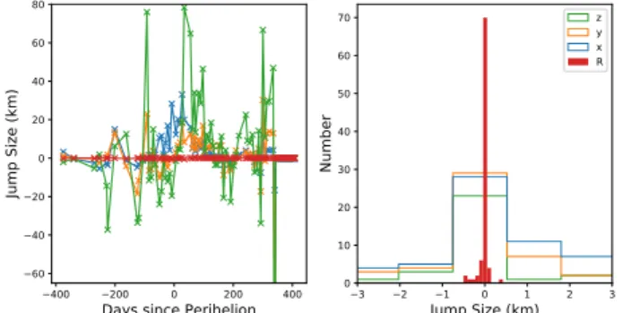
Theoretically, the NGA resulting from outgassing could be directly extracted from the residuals between this mea-sured trajectory and a modelled gravitational orbit (taking into account general relativity and the gravitational accel-erations of all major planets, Pluto and the most massive asteroids). During the course of this work, however, it was discovered (and later confirmed by ESAC; B. Grieger, per-sonal communication) that the reconstructed comet and spacecraft trajectories contain a series of discontinuities, at which the objects’ positions vary over hundreds of metres to several kilometres in an instantaneous time, making the above method impossible. Within the orbital segments be-tween these ‘jumps’, there is no difference, to machine preci-sion, between our own orbital integrations (see Sect. 3.2 be-low) and the reconstructed trajectory, demonstrating that it is a purely gravitational solution. The jumps occur at the boundaries between the integration segments that make up the reconstructed orbit, and represent the offset in the ob-jects’ positions over the course of each segment due to the un-modelled non-gravitational acceleration. Unfortunately, it proved impossible to extract the NGAs directly from the jumps themselves as they contain, not only, the NGA ef-fect but also the typical uncertainty in the state vector at the start of each segment, which is of a comparable mag-nitude. The jumps therefore have random magnitudes with time (Fig. 1) and must be considered an additional source of noise in the uncertainty in the measured positions.
Despite these issues, the reconstructed kernels remain a good description of the comet’s trajectory over orbital timescales, and within the limits of accuracy of the typical jump size. Therefore it is still possible to compare these measurements with a model of the orbit, including a ther-mal outgassing NGA as well as N-body gravitational inter-actions, in order to constrain said model. To do so, we use the magnitude of the comet-to-Earth-centre range as our observable OR, since the jump sizes are smallest in this
di-rection (Fig. 1). Considering the jumps to be a source of random error, we conservatively estimate the uncertainty in OR as R⇡ 1 km.
2.3. Rotation
Back-reaction from outgassing not only produces a net ac-celeration on the nucleus but can also, depending upon its shape, produce a net torque, altering its rotation state. The rotational parameters of 67P, including its spin rate over time, !(t), has been measured as part of the reconstruction of its 3D shape from OSIRIS images (Jorda et al. 2016).
Fig. 1. Discontinuities identified in the position of comet 67P from the SPICE kernels, in (x, y, z) heliocentric J2000 coordi-nates and Earth-comet range (R). On the left: as a function of time and on the right as a histogram of sizes.
Fig. 2. Observed torque, derived from the 67P rotation state from OSIRIS measurements, and a smoothed cubic spline fit to the data. The grey region represents the RMS of the residuals between the two.
After verifying that the cross terms relating to the an-gular velocities along the first and second principal axes of the comet are negligible, changes in spin rate, ˙!z, can be
directly related to the z component of the torque (⌧z, in
a body-fixed frame) by Eq.(1), where Iz = 1.899⇥ 1019
kg m2is the third (largest) moment of inertia derived from
the shape model assuming a constant density of 538 kg m 3
(Preusker et al. 2017).
⌧z⇡ Iz!˙z, (1)
Differentiating the observed !(t) by time exacerbates mea-surement uncertainties so that the produced torque curve becomes extremely noisy. For comparing with our simula-tions below, we therefore smooth the data by fitting it to a cubic spline, as shown in Fig. 2. Our fitted spline is then used as the torque observable, O⌧, with an assumed
un-certainty equal to the root mean squared residuals of the derived minus smoothed data, ⌧ = 575000 N.m(shown in
3. Modelling
3.1. Thermal model
A thermal model is required to compute the temperature of the sublimating layer (assumed to be at the surface on the nucleus), from which we can derive the non-gravitational forces acting on the nucleus. Our thermal model takes into account solar insolation, surface thermal emission, subli-mation of water ice, projected shadows and self-heating. We use a decimated version of the 67P shape model called SHAP7 (Preusker et al. 2017), with 124 938 facets. The temperature is computed for each facet of the shape model, 36 times per rotation (i.e., every 1240 s), and 70 times (i.e., every ⇠ 10 days) over the 2 years of the Rosetta mission, to ensure a good temporal coverage. At each time step, the distance to the Sun, the orientation of each facet rela-tive to the Sun, and the projected shadows, are computed using the OASIS software (Jorda et al. 2010). Due to the large number of facets (>100 000) and time steps (>2500), heat conduction is neglected in the thermal model for nu-merical reasons. To test this assumption, we computed the production rate (Eq. 4) and acceleration (Eq. 5) of a spher-ical nucleus, at perihelion (where the torque is maximum), for two cases: a thermal inertia of 0 and 100 J/m2/K/s0.5.
The production rate and the acceleration are ⇠7 % smaller for a thermal inertia of 100 J/m2/K/s0.5 (compared to a
null thermal inertia), and the direction of the acceleration vector differs by less than 3 deg. Neglecting the thermal inertia therefore appears reasonable compared to the data uncertainties (e.g., production rates).
The surface energy balance of the thermal model is given by Eq. (2), for a facet with index i, where Ab= 0.0119is the
Bond albedo at 480 nm (Fornasier et al. 2015), Fsun= 1370
W/m2 is the solar constant, z
i is the zenithal angle, rh
the heliocentric distance, SHi is the self-heating given by
Eq. (3), ✏ = 0.95 is the assumed infrared emissivity, Ti is
the surface temperature, fi is the fraction of water ice (in
our case, either 0 for pure dust or 1 for pure ice, see below), ↵ = 0.25 accounts for the recondensation of water ice on the surface (Crifo 1987), L = 2.66 ⇥ 106J/Kg is the latent
heat of sublimation of water ice at 200 K, and Zi is the
water sublimation rate given by Eq. (4). (1 Ab)Fsuncos zi
r2 h
+ SHi= ✏ Ti4+ fi(1 ↵)LZi(Ti) (2)
In Eq. (3), the self-heating SHi is the sum of the infrared
flux coming from all the n facets with index j that see facet i, where Sjis the surface of facet j, ✓jthe angle between the
normal to facet j and the vector joining facets i and j, ✓ithe
angle between the normal to facet i and the vector joining facets i and j, and d2
ijis the distance between facets i and j.
This formalism is similar to that of Gutiérrez et al. (2001). To look for which facets are seeing each others, we used an algorithm developed at Laboratoire d’Astrophysique de Marseille based on ray tracing and hierarchical search. The computation of the viewing factors (Sjcos ✓jcos ✓i)/(⇡d2ij)
is purely geometric and depends only on the shape model: it is therefore only performed once at the beginning.
SHi= n X j=0 ✏ Tj4 Sjcos ✓jcos ✓i ⇡d2 ij (3)
In Eq. (4), the sublimation mass flow rate per facet is calcu-lated with the molar mass M = 0.018 kg, the two constants A = 3.56⇥ 1012 Pa and B = 6162 K for water (Fanale &
Salvail 1984), and the gas constant R = 8.3144598 J K 1
mol 1.
Zi= Ae B/Tice
r M
2⇡RTice (4)
Finally, to compute the non-gravitational forces (Sect. 3.2), we need the sublimation rate (Eq. (4)) and the gas velocity (Eq. (6)), which both depend on a different temperature: the temperature of water ice Tice for Zi, and the
temper-ature of dust Tdust for vi. We therefore run our thermal
model (Eqs. (2) to (4)) with two extreme cases: [1] with fi = 0, which corresponds to a pure dust model, to
com-pute Tdust, and [2] with fi= 1, which corresponds to a pure
water ice model, to compute Tice.
3.2. Non-Gravitational Force model
The reaction force vector per facet is then calculated based on this mass flow rate, and the total acceleration is the sum over all facets divided by the comet mass (M67P =
9.982⇥ 1012 kg; Pätzold et al. 2016): Fi= ⌘xiZiviSi, aN G= P iFi M67P . (5)
where ⌘ is the momentum transfer coefficient (Crifo 1987; Rickman 1989), which we here assume to be con-stant across the comet. Si is the surface area of each facet
(in the direction of its normal) and xi is its effective active
fraction. Mass flow rate is calculated with Eq. (4) and the gas velocity is taken as the thermal velocity
vi=
r
8RTdust
⇡M , (6)
assuming equilibrium with the surface grey body tempera-ture, i.e. that of the dust from run [1] of the thermal model. This is the upper limit that the gas can reasonably reach, meaning our non-gravitational force will be on the high end of estimation and our effective active fractions are lower lim-its. Calculated dust temperatures range between ⇠ 20 390 K (ice temperatures are limited by the sublimation to ⇠ 200 K), leading to thermal velocities of ⇠ 155 658 m s 1.
Water production and torque are likewise summed over the surface Q =X i xiZiSi. ⌧N G= X i ⌧i, (7)
where torque per facet is the vector product of each force vector with its radius vector to the centre of mass (ri). This can also be expressed as the magnitude of the
force multiplied by a “torque efficiency” (see Keller et al. 2015):
⌧i= ri⇥ Fi= Fi(ri⇥ ˆSi). (8)
The z component of the total net torque can then com-pared with the observations, using Eq. (1). It is advanta-geous to use the torque efficiency formalism since this vector is in the body-fixed frame, and can be calculated once at
+X
+Z
+Y -Y
-Z -X
Fig. 3. Torque efficiency in metres, a factor determined by the geometry as defined in Eqn. 8. The comet’s rotation axis is in the +z direction through the ‘neck’ region in the centre.
the beginning of the simulation run, rather than being re-calculated each time. Torque efficiency is also a useful way of visualising the effects of differing spatial distributions in activity, which will be important later during the opti-misation. Mapping torque efficiency onto the shape model (Fig. 3) shows how local variations in topography combine with large scale orientations of regions, varying the effects of activity on the comet’s rotation across its surface (com-pare with Fig. 1 in Keller et al. 2015, which uses an older, incomplete shape model that is missing the southern hemi-sphere).
Non-gravitational forces are calculated for each of the 70⇥ 36 = 2520 runs of the thermal model and the relevant quantities (force and torque vectors and summed water pro-duction) are averaged over a day. This produces smoothly time-varying curves which can be inspected at any time of interest, using bilinear interpolation, which we refer to as our model solution. For comparison with the observed wa-ter production rate and torque, we can simply evaluate our model at the time of each measurement, producing CQ and
C⌧, and directly compare.
For the trajectory, however, a full N-body integration must be performed and the resulting position compared at each time (CR). To do this we use the open-source
REBOU N D code1 (Rein & Liu 2012), complete with full general relativistic corrections (Newhall et al. 1983) as im-plemented by the REBOUNDx extension package2. All
the major planets are included, as well as Ceres, Pallas,
1 http://rebound.readthedocs.io/en/latest/
2 http://reboundx.readthedocs.io/en/latest/index.html
and Vesta, and are initialised with their positions in the J2000 ecliptic coordinate system according to the same ephemerides used in the Rosetta trajectory reconstructions (NASA/JPL solar system solution DE405; Standish 1998). An additional particle representing 67P is initialised with its position given by SPICE. The system is then integrated forward in time, using the IAS15 integrator (Rein & Spiegel 2015) and the standard equations of motion, with the ad-dition of a custom acceleration, aN G, for 67P, provided by
our model. The modelled comet begins to diverge from the measured positions and at each time of interest we directly compare the magnitudes of the computed and measured comet-to-Earth-centre ranges, R (the most accurate part of the trajectory as described in sect. 2.2 above).
3.3. Optimisation
In order to constrain the unknown parameters in our model, such as the the surface active fraction, we perform a bounded least-squares fit to the data using the dogleg optimisation routine (Voglis & Lagaris 2018) provided in the scientific Python package. The optimisation proceeds, attempting to minimise the standard objective function
Obj = N X j=0 ✓ Oj Cj j ◆2 , (9)
with observed minus computed residuals, O C, and ob-servation uncertainties, , at each time-step, j, up to the total N. The root mean squared residuals are then RMS = p
Obj/N.
In our case we have three separate datasets to fit to (R, Qand ⌧), a multi-objective optimisation problem, and we therefore use a linearly-scaled combination of the three to generate a combined objective function. The term inside the brackets in Eq. (9) then becomes the sum of the three terms R ✓O Rj CRj Rj ◆ , for 0 < j NR, Q ✓ OQj CQj Qj ◆ , for NR< j NR+ NQ, ⌧ ✓ O⌧ j C⌧ j ⌧ j ◆ , for NR+ NQ< j N, (10)
respectively, where N = NR+ NQ+ N⌧ runs over the
combined number of points in all three datasets, and the scaling coefficients are variables, which themselves must be optimised in order to give the desired weighting to each dataset. We set R= 1and scale the other lambdas relative
to it, by bootstrapping from the residuals of a preliminary run, to give roughly equal weighting to all three datasets. Due to the very small relative errors for range ( R/R⇠ ±1
km /1 AU), this results in large values for the other lambdas ( Q ⇠ ⌧ ⇠ 50) to give equal weighting.
For each optimisation, we fix the coupling factor, ⌘, at a constant value and parametrise the model in terms of effective active fraction, x, across the surface. The effects of ⌘ on the best-fit model can then be studied indepen-dently. To begin with, we use the division of 67P’s surface into five ‘super regions’, as performed by Marschall et al. (2016, 2017) in fitting ROSINA/COPS and OSIRIS data,
+Z -Z
Fig. 4. Map of the 5 ‘super regions’ defined by Marschall et al. (2016, 2017) and used in our solution A optimisation.
and start the optimisation with initial values from their re-sults. This divides the comet into: a southern hemisphere region, an equatorial region, a region covering the base of the body and top of the head, Hathor, and Hapi, as shown in Fig. 4 below. The fitting routine then proceeds to optimise these five free parameters, subject to the lower and upper boundaries of zero and one, i.e. 0 100% active fraction. As described below, we also use more detailed parameteri-sations, including all 26 regions of Thomas et al. (2015) for 26 free parameters.
4. Results
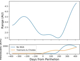
Before optimising our activity model we first test the N-body component by calculating the comet trajectory over the course of the Rosetta mission with no NGAs applied, and with the classic NGA parametrisation based on the model of Marsden et al. (1973). This model computes the three components of aN G (radial, along-orbit and
normal-to-orbit) based on a power-law with heliocentric distance, and three scaling parameters A1,2,3found by a formal
best-fit to the orbit for each comet. We use the A1,2,3 values for
the 2010 apparition of 67P from ground-observations given by NASA/JPL Horizons ephemerides3.
Figure 5 shows a plot of the observed range plus the residuals to both models. The RMS residuals are 1029 km and 675 km, respectively, showing the order of magnitude of the accuracy of the Marsden et al. (1973) model with ground-based observations of roughly arcsecond accuracy. This stands as a baseline, against which we can check our own activity model.
4.1. 5 parameter solution (A)
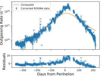
Figures 6 –8 show the residuals to our best-fit solution using the five super regions defined by Marschall et al. (2016, 2017), which we refer to as our solution A.
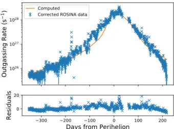
The RMS range residuals, of 163 km (see Table 1 for all results), represent a significant improvement over the ⇠ 1000 km of the purely gravitational solution and the ⇠ 600 km of the ground-based solution, demonstrating the significance of our NGA/N-body model. However, the water production curve is clearly not a good fit, failing to repro-duce both the peak production rate as well as overestimat-ing the production far from perihelion. Likewise, the torque curve is an extremely bad fit, failing totally to reproduce the expected positive torque peak (spin up) at perihelion.
3 https://ssd.jpl.nasa.gov/?horizons
Fig. 5. Observed Earth-comet range, R, and residuals for two models: a purely gravitational N-body solution with no NGA, and a ground-based solution based on the model of Marsden et al. (1973) (see text for details). Differences between the ob-served and computed solutions, as well as the jumps described in Sect 2.2, are invisible at the scale of the top plot.
Fig. 6. Observed minus computed range, R, for solution A (blue curve). For comparison, the residuals to the ground-based solu-tion, using the Marsden et al. (1973) model as in Fig. 5, are shown in orange. Both curves diverge from zero most sharply following the maximum perturbation around perihelion, but our solution is an improvement.
This is confirmed by the RMS (normalised) residuals of 6.59 and 5.13, respectively.
Figure 9 shows the active fractions for this solution, mapped onto the shape model. Some artefacts of the region definition can be seen, introducing spurious active fractions at the borders between regions, but these facets represent a small fraction of the total area and should not influence the general results. A large difference between the effective active fractions in the northern and southern hemispheres can be seen in Fig. 9, with the southern hemisphere show-ing active fractions of up to 12%, while the north is only a few percent active. This is supported by previous works (Marschall et al. 2016, 2017) based on the interpretation of ROSINA data. It is also consistent with the higher active
Solution ⌘ R Q ⌧ RMSR(km) RMSQ RMS⌧ RMSObj No NGA 1029 1029 Ground-based 675 675 A 0.7 1 50 50 163 6.6 5.1 259 B 0.7 1 50 50 187 5.2 2.1 235 C 0.7 1 50 50 46 4.2 0.57 125 Ca 0.5 1 50 50 115 5.5 1.32 176 Cb 0.6 1 50 50 64 4.3 0.61 130 Cc 0.8 1 50 50 62 5.5 1.52 168
Table 1. Parameters and root-mean-squared residuals (in range, water production rate, non-gravitational torque, and the total objective function) for the best-fit models. ‘No NGA’ is an N-body only model computed in REBOUND, while ‘Ground-based’ has an additional force given by the Marsden et al. (1973) model with parameters from NASA Horizons. A, B and C use the thermal model described here. The best model (C) is highlighted in bold font.
Fig. 7. Observed and computed water production rates and residuals for solution A.
Fig. 8. Observed and computed torques and residuals for solu-tion A.
fraction (up to a factor of 2–3 in the southern hemisphere compared to the northern hemisphere) found by (Kramer et al. 2019) from a thorough study of the evolution of the rotational parameters of 67P. The southern regions of comet 67P receive higher insolation during southern
sum-+Z -Z
Fig. 9. Mapped active fraction for solution A.
mer which occurs near perihelion: the summer solstice hap-pens on Aug 15, 2015, only a couple of days after perihelion. An analysis of OSIRIS images of the Anhur/Bes south-ern regions (Fornasier et al. 2017) shows a high activity originating from these regions, combined with high relative erosion rates deduced from the relatively higher number of boulders found (Pajola et al. 2016). An examination of the production and force curves produced by the individual super regions showed that the southern hemisphere domi-nates production after equinox and around perihelion, as expected. Taken as a whole, the southern hemisphere has a negative torque efficiency (see Fig. 3), which leads to the difficulty in jointly fitting both the production and torque curves, seen in our solution A residuals. Splitting the south-ern hemisphere into more regions is therefore a promising next step.
4.2. 26 parameter solution (B)
Figures 10 –12 show the residuals to our optimisation with the full 26 comet regions defined by Thomas et al. (2015), which we refer to as our solution B.
Figure 12 shows a clear improvement in how well we fit the torque peak, with the model now showing a posi-tive peak of roughly the right magnitude, although still not matching the shape. The improved RMS residual of 2.09 backs this up. Conversely, however, the range residuals are now slightly increased, relative to solution A, and the water production curve is still not well fitted; peak production in
Fig. 10. Observed minus computed range for solution B (blue curve), and the ground-based solution.
Fig. 11. Observed and computed water production rates and residuals for solution B.
Fig. 12. Observed and computed torques and residuals for so-lution B.
+Z -Z
Fig. 13. Mapped active fraction for solution B.
the model is still too low, and does not fall off fast enough with heliocentric distance post-perihelion.
The active fraction map of Fig. 13 shows the same trend for high activity in the southern super-regions as before but now with slightly higher activity in Hapi, matching Marschall et al. (2016). Active fraction in the southern re-gions can be seen to vary significantly and it is instructive to compare this distribution to the map of torque efficiency. As can be seen from Fig. 3, positive torque efficiency is clustered in several small areas, and these are given high activity by our optimisation. However, the optimisation is limited by the fact that the geographically defined regions containing these areas also contain areas of negative torque efficiency. In other words, torque efficiency varies at a local scale and is not necessarily correlated with the regions used in this parametrisation.
To address this, we could further subdivide our regions, introducing more parameters, but no obvious best way to do this presents itself. Instead we take the, somewhat simpli-fied, approach of reverting back to the 5 super region model of solution A, and simply splitting the southern super re-gion by torque efficiency. This creates two non-contiguous and “spotty” super regions, which do not necessarily corre-spond to particular morphological or structural regions on the cometary surface, but do provide a parametrised way of optimising the NGA model. Experiments with this method show significant improvements over models A and B, but still have problems reproducing the production rate curve, which we address in the next subsection.
4.3. Time-varying solution (C)
Since the above solutions with constant active fractions fail to adequately reproduce all the data, we now consider time-varying solutions. Temporal variations of the effective active fraction is an obvious way to try to reconcile the modelled post-perihelion slope of the water production rate with the measured data.
We begin with the 6 super regions (including a south-ern hemisphere split by torque efficiency) and implement a time-varying active fraction for both the southern hemi-sphere regions (since these are the most important around perihelion) while keeping the others constant. We first con-sidered a decline of the active fraction with time, with a half-Gaussian fall-off from the initial value, fitting for both the active fractions and start and decay times of the
Gaus-Fig. 14. Observed minus computed range for solution C (blue curve), and the ground-based solution.
sian. While this produced encouraging results, it is a some-what unphysical situation: the comet’s orbit is cyclical so that the active fraction must “reset” back to the initial value in time for the next perihelion. This may happen slowly around aphelion, in which case it will not affect the fit here, or it may occur during the time-period studied by Rosetta. To explore this latter case, we perform a final optimisation, allowing two active fractions for each of the two southern hemisphere regions as well as two start times, t0 and t1,
and two decay (or growth) half-times, t1
20 and t 1 21, for a
total of twelve fitted parameters. The relative magnitudes of the two active fractions are unconstrained, but the two times, t0and t1, are constrained to lie either side of
perihe-lion to ensure that they do not cross over. The half-times are constrained to be larger than zero but unconstrained at the top end.
Finally, we also vary the momentum transfer efficiency (⌘ parameter) around our nominal value ⌘ = 0.7. A full op-timisation of the twelve parameters is performed adopting ⌘ values of 0.5, 0.6 and 0.8 (models Ca, Cb and Cc in Table 1). As shown in Table 1, the smallest multi-objective function (Eq. (3.3)) is achieved for ⌘ = 0.7, with a minimum value of 124. While the ⌘ = 0.5 and ⌘ = 0.8 solutions correspond to a significantly higher multi-objective function (equal to 175 and 168, respectively), the ⌘ = 0.6 solution (equal to 130) is only marginally larger.
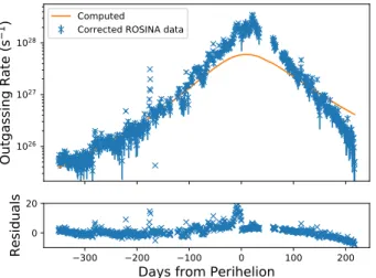
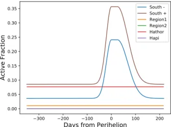
Figures 14 –16 show the residuals for our best fit model in this case: model C, while Figs. 17 and 18 show the mapped (peak) active fraction distribution and how it varies with time. High activity is again favoured in the southern regions, with the optimisation now selecting very high effective active fractions, of over 35%, in order to fit the high peak production rates at perihelion (Fig. 15). Higher active fractions in areas producing a positive torque allow them to dominate the rest of the southern hemisphere, pro-ducing a net positive torque curve, which now matches very well the observations (Fig. 16). Note however that the small drop off observed 125 days before perihelion is not repro-duced by the model.
Figure 18 shows that the preferred solution has south-ern active fractions increase quickly between equinox and perihelion (with a half-time of ⇠ 25 days) to their high
Fig. 15. Observed and computed water production rates and residuals for solution C.
Fig. 16. Observed and computed torques and residuals for so-lution C.
peak values, before falling off to the ⇠ 10% level after peri-helion and during southern summer, with a decay half-time of around 50 days. This reproduces the high production rate at perihelion while matching the swift fall-off over the
+Z -Z
Fig. 18. Active fraction with time for solution C.
succeeding two hundred days. Some discrepancies with the data still remain, for example the “knee” feature seen as the production ramps up around a hundred days before perihe-lion, but the result is now a much better match to the data overall.
The greatly reduced range residual, of 46 km, is further evidence of the improved model, and confirms that the ma-jority of the NGA effect is concentrated near perihelion. The fact that non-gravitational forces and production are both seen to be strongly peaked near perihelion, over and above what one would expect from geometric considerations, is consistent with a time-varying active fraction. Small dif-ferences seen in the torque and production curves occur before equinox, when outgassing is controlled by the active fraction in the Northern hemisphere, which we do not vary with time. This suggests that minor improvements might be made to the fit by focusing on the North, although these would be unlikely to affect the trajectory and peak produc-tion, both of which are dominated by activity at perihelion (i.e. in the South).
The best-fit results allow us to calculate integrated quantitative parameters resulting from the cometary ac-tivity around perihelion. The total water ice mass loss amounts to 4.5 106 kg, corresponding to a mean erosion
of ⇠ 9 cm over the entire nucleus surface, assuming a den-sity of 538 kg m 3 (Preusker et al. 2017). We emphasize
that this estimate does not take into account the dust mass loss - predicted to be much larger depending on the dust-to-ice ratio - and the outgassing of more volatile minor species throughout the orbit. The actual water ice erosion can be calculated by integrating the time-varying sublimation rate of each facet. We find a local erosion of 0.4 1.4 m in the two southern super-regions and < 0.1 m in the northern ones.
5. Discussion
5.1. A temporal variation of the effective active fraction The most striking features of our best solution (C) are the dichotomy of the effective active fraction between the south-ern and northsouth-ern hemispheres on the one hand, and the drastic rise of the effective active fraction around perihe-lion in the southern regions on the other hand. The latter
is required in our approach to explain the steep slope of the production rate. We propose the following qualitative ex-planation, based on the seasonal formation and disappear-ance of a dust mantle, for this cyclic increase of effective active fraction in the southern regions around perihelion. This idea has been introduced a long time ago in the liter-ature. Among the pioneering works, Brin & Mendis (1979), Brin (1980) and Fanale & Salvail (1984) introduced the idea that a dust mantle can form and be subsequently disrupted by the gas pressure if it remains thin enough. Using a one-dimensional thermal model, Rickman et al. (1990) showed how the obliquity of the spin axis can influence the stabil-ity of the mantle. They show that a temporary mantle can form at intermediate and polar latitudes for nuclei with radii equal to 5 km and high obliquities (equal to 90 in their simulations). For nuclei with smaller radii (equal to 1 km), temporary mantles only appear at perihelion dis-tances smaller than 1 a.u.. In a more recent work based on a 3D thermal model, De Sanctis et al. (2010) tried to repro-duce the thermal evolution of 67P. The role of the obliquity is emphasized as being critical, high obliquities favouring the appearance of a stable dust mantle at equatorial lati-tudes. Other models (e.g., Kossacki & Szutowicz 2006) find on the contrary that a stable mantle with a non-uniform dust layer can explain the observed water production rates. In our explanation, the southern regions - including the southern polar cap - become progressively illuminated and the activity starts to increase after the spring equinox (93 days before perihelion – 11 May 2015). This rise of ac-tivity allows dust present at the surface to be lifted off, decreasing the depth at which water ice is present below the dust layer. This is a runaway process as the increased gas flux resulting from this reduced dust depth is able to lift off larger and larger dust particles from the surface. An increasing fraction of these particles eventually reaches ve-locities large enough to escape the nucleus gravity, or to be redeposited in other nucleus (Northern) regions. This mechanism leads to an increase of the effective active frac-tion. After the summer equinox (3 days after perihelion – 15 August 2015), the energy input starts to decrease, re-sulting in a reduced gas flux and surface temperature. The large dust particles can no longer be lifted off from the sur-face and start to be redeposited locally. The apparition of a dust mantle quenches the cometary activity as the water is no longer at the surface of the comet; instead, it subli-mates through a deeper dust layer beneath the surface. The gas diffusion through this dust mantle produces lower gas fluxes, decreasing the effective active fraction of the surface. The process continues for several months until the autumn equinox (224 days after perihelion – 24 March 2016) trig-gers the southern autumn, followed by the long southern winter around aphelion. At that time, the southern regions are covered again by a dust layer that will be partially removed at the next perihelion passage. It is not totally excluded also that the outgassing of more volatile species during the northern summer at aphelion contributes to the re-accumulation of material in the southern hemisphere.
This scenario is partially supported by observations from instruments aboard Rosetta. Lai et al. (2016) mod-elled the dynamics of dust grains around 67P taking into account OSIRIS observations. They predict that dust par-ticles ejected from the southern hemisphere are redeposited in the northern hemisphere during the southern summer. A recent geomorphological analysis of the surface (Birch et al.
2017) also supports the hypothesis of dust being ejected from the southern hemisphere and redeposited in the north-ern regions, as do several other works such as Thomas et al. (2015); Keller et al. (2017) and Hu et al. (2017). Finally, Fornasier et al. (2016) observed seasonal variations of the colour of the nucleus, which becomes bluer near perihelion. This colour change is attributed to the removal of the dust mantle covering regions with low gravitational slopes as the comet approaches perihelion.
It must be noted that our model interprets active area as a literal fraction of the surface area which is covered with water ice and is outgassing. Since exposed water ice is rare on the surface, this is a simplification of the real process, which should involve gas flow through pores, dust layers, erosion etc., the details of which we consider beyond the scope of this paper. Nonetheless, effective active fraction is a useful proxy with which to quantify activity, with the above-noted spatial and temporal variations providing an insight into the changing activity patterns over the comet’s seasons. Our area-weighted global average values, of 6.4% around perihelion and 1.9% otherwise, agree well with pre-vious estimates for 67P (Lamy et al. 2007) and other comets (see, e.g. A’Hearn et al. 1995), but the large differences be-tween hemispheres and seasons highlights the limitations of interpreting cometary activity with a single number from the ground.
5.2. A refined value for the ⌘ parameter
The ⌘ parameter, also called “momentum transfer effi-ciency” in the literature represents the fraction of the Maxwellian thermal velocity of the gas, calculated from the nucleus surface temperature, contributing to the mo-mentum transfer. This parameter depends on the local ice content and on the detailed structure of the porous mate-rial. Its value couples the water production curve with the effect of the spin/orbit variations, allowing to compensate any systematic effect possibly present in the input data or in the model. The value of the ⌘ parameter has been calculated from gas-kinetic models of the Knudsen layer. Delsemme & Miller (1971) adopted a value ⌘ = 0.6, between the pure ice plane surface value ⌘ = 1/2 and higher values up to 2/3 predicted for porous media. In early interpretations of the NGA of comet 1P/Halley, Rickman (1986) and Sagdeev et al. (1988) used a value of 0.5 and 0.79 respectively based on different assumptions. Crifo (1987) recommended a value ⌘⇡ 0.5 based on revised gas-kinetic theoretical description of the solid-gas interface, taking into account the recon-densation of water ice. Rickman (1989) used a corrected value ⌘ = 0.53 0.67 based on the work of Crifo (1987), which seem to be in good agreement with gas velocity mea-surements in the coma of comet 1P/Halley (see Rickman 1989, and references therein). However, the calculations do not consider intimate ice-dust mixtures and do not take into account the porosity of the surface. Skorov & Rickman (1999) introduced a correction factor of 1.8 to the values adopted by Rickman (1989) based on an analytical model of the Knudsen layer above a porous dust mantle. This leads to very high ⌘ values in the range 1 1.2.
From our analysis of the data presented in this paper, our best fits are obtained for ⌘ in the range 0.6 0.7, in good agreement with the moderate values adopted in the liter-ature. They do not support more extreme values (around 0.5 and greater than 0.8), which degrade the overall fit of
the three data sets. We stress however that we set the sur-face gas temperature to the dust temperature Tdust in our
model (see Eq. (6)). This may lead to overestimating the gas temperature, which would in turn tend to underesti-mate the fitted value of ⌘. Note, however, that the depen-dence of the gas velocity with the temperature is a square root in Eq. (6): a large and constant temperature devia-tion would be needed to significantly bias the value of ⌘. The second point of concern is a possible overestimate of the water production curve due to sublimating icy grains in the coma. This would once again require a larger value of ⌘ to compensate the smaller local sublimation rates. Alto-gether, even if our simulations point to ⌘ < 0.8 we cannot entirely rule out at this point higher values of this param-eter. Consolidated values of the surface water production around perihelion, as well as estimates of the gas velocity above the surface, would help to reduce the uncertainties.
6. Conclusions and perspectives
From our work, the following conclusions could be reached: 1. We succeeded in finding an activity pattern explaining simultaneously the three following 67P data sets, ex-tracted mainly from the Rosetta mission: (1) the Earth-comet ranging data reconstructed by the flight dynam-ics team of ESA/ESOC, (2) the water production rate deduced from a mix of ROSINA and ground-based ob-servations (Hansen et al. 2016), and (3) the rate of spin period change deduced from the OSIRIS images. The residuals of the ranging data describing the effect of the non-gravitational acceleration are reduced by an order of magnitude compared to the ground-based solution based on the simple model of Marsden et al. (1973). 2. The fitted activity pattern exhibits two main features:
a higher effective active fraction in two southern super-regions (⇠ 10 %) outside perihelion compared to the northern ones (< 4 %), and a drastic rise of the effective active fraction of the southern regions (⇠ 25 35 %) around perihelion.
3. In order to successfully fit the positive rate of spin pe-riod change, we need to split the southern super region into two entities, depending on the sign of the torque ef-ficiency. These two entities correspond to two relatively well delimited areas in Anhur, Bes and Khepry, but cre-ates a patchy separation in Wosret.
4. We interpret the time-varying southern effective active fractions by cyclic formation and removal of a dust man-tle in these regions. According to our interpretation, the dust mantle could be progressively removed when activ-ity rises after the southern spring equinox and formed again when activity decreases towards the southern au-tumn equinox (and possibly around aphelion during the northern summer). Several observations performed dur-ing the Rosetta mission, such as dust transport from South to North (Lai et al. 2016; Birch et al. 2017) and bluer colours observed near perihelion (Fornasier et al. 2016), support this interpretation.
5. If it is confirmed, this interpretation would strongly support post-Halley thermal modelling (Rickman et al. 1990; De Sanctis et al. 2010) which predicted that sea-sonal effects linked to the orientation of the spin axis play a key role in the formation and evolution of dust mantles, and in turn largely control the temporal vari-ations of the gas flux.
6. Our analysis supports moderate values of the momen-tum transfer coefficient ⌘ in the range 0.6 0.7. For more extreme values of this coefficient ( 0.5 and 0.8), the fit of the three data sets is degraded. However, we will not be able to rule out higher values of this parameter without consolidated water production measurements and, to a lesser extent, without estimates of the near-surface thermal gas velocity.
More work will be needed to better understand the ac-tivity of 67P using data collected during the Rosetta mis-sion. The solution found in this article through the pro-cess described in section 4 is non-unique on the one hand, and could probably be improved on the other hand. Im-provements may come from a better understanding of the ranging data, resulting in the extraction of clean and accu-rate non-gravitational acceleration of the comet as a func-tion of time around perihelion. The change in the direcfunc-tion of the spin axis or angular velocity could also provide a valuable additional data set that could help to constrain the activity pattern and reduce the number of solutions. In their interpretation of the temporal evolution of the rota-tional parameters, Kramer et al. (2019) did not introduce a temporal variation of the activity around perihelion but considered instead a spatially heterogeneous surface with 36 “patches” having different water-ice coverage. They also discuss the possibility of a decreasing dust layer near perihe-lion increasing activity, and found a solution explaining the water production curve of 67P. It would be interesting to test if this solution could also reproduce the NGA of comet 67P described in this article. Finally, a better understand-ing of the production rate around perihelion, reconcilunderstand-ing the different Rosetta instrument measurements and includ-ing species other than water, would be of benefit in fittinclud-ing the activity model.
Acknowledgements. This project has received funding from the Euro-pean Union’s Horizon 2020 research and innovation programme under grant agreement no. 686709. This work was supported by the Swiss State Secretariat for Education, Research and Innovation (SERI) un-der contract number 16.0008-2. The opinions expressed and arguments employed herein do not necessarily reflect the official view of the Swiss Government. We thank the authors of several python pack-age libraries which were used extensively here; these include NumPy, SciPy, SpiceyPy, REBOUND and REBOUNDx. We are grateful to L. Maquet for fruitful discussions in the course of this work. We also thank the reviewer, Dennis Bodewits, for his comprehensive and useful review.
References
Acton, C. H. 1996, Planet. Space Sci., 44, 65
A’Hearn, M. F., Millis, R. C., Schleicher, D. O., Osip, D. J., & Birch, P. V. 1995, Icarus, 118, 223
Bertaux, J.-L. 2015, A&A, 583, A38
Birch, S. P. D., Tang, Y., Hayes, A. G., et al. 2017, MNRAS, 469, S50 Bodewits, D., Farnham, T. L., Kelley, M. S. P., & Knight, M. M.
2018, Nature, 553, 186 Brin, G. D. 1980, ApJ, 237, 265
Brin, G. D. & Mendis, D. A. 1979, ApJ, 229, 402 Crifo, J. F. 1987, A&A, 187, 438
Davidsson, B. J. R. & Gutiérrez, P. J. 2004, Icarus, 168, 392 Davidsson, B. J. R. & Gutiérrez, P. J. 2005, Icarus, 176, 453 Davidsson, B. J. R. & Gutiérrez, P. J. 2006, Icarus, 180, 224 Davidsson, B. J. R., Gutiérrez, P. J., & Rickman, H. 2007, Icarus,
191, 547
De Sanctis, M. C., Lasue, J., Capria, M. T., et al. 2010, Icarus, 207, 341
Delsemme, A. H. & Miller, D. C. 1971, Planet. Space Sci., 19, 1229 Drahus, M. & Waniak, W. 2006, Icarus, 185, 544
Fanale, F. P. & Salvail, J. R. 1984, Icarus, 60, 476
Fornasier, S., Feller, C., Lee, J.-C., et al. 2017, MNRAS, 469, S93 Fornasier, S., Hasselmann, P. H., Barucci, M. A., et al. 2015, A&A,
583, A30
Fornasier, S., Mottola, S., Keller, H. U., et al. 2016, Science, 354, 1566 Gutiérrez, P. J. & Davidsson, B. J. R. 2007, Icarus, 191, 651 Gutiérrez, P. J., de León, J., Jorda, L., et al. 2003, A&A, 407, L37 Gutiérrez, P. J., Jorda, L., Samarasinha, N. H., & Lamy, P. 2005,
Planet. Space Sci., 53, 1135
Gutiérrez, P. J., Ortiz, J. L., Rodrigo, R., & Ló pez-Moreno, J. J. 2001, A&A, 374, 326
Hansen, K. C., Altwegg, K., Berthelier, J.-J., et al. 2016, MNRAS, 462, S491
Hu, X., Shi, X., Sierks, H., et al. 2017, A&A, 604, A114 Jorda, L., Gaskell, R., Capanna, C., et al. 2016, Icarus, 277, 257 Jorda, L., Spjuth, S., Keller, H. U., Lamy, P., & Llebaria, A. 2010, in
Proc. SPIE, Vol. 7533, Computational Imaging VIII, 753311 Keller, H. U., Delamere, W. A., Reitsema, H. J., Huebner, W. F., &
Schmidt, H. U. 1987, A&A, 187, 807
Keller, H. U., Mottola, S., Hviid, S. F., et al. 2017, MNRAS, 469, S357 Keller, H. U., Mottola, S., Skorov, Y., & Jorda, L. 2015, A&A, 579,
L5
Knight, M. M., Farnham, T. L., Schleicher, D. G., & Schwieterman, E. W. 2011, AJ, 141, 2
Kossacki, K. J. & Szutowicz, S. 2006, Planet. Space Sci., 54, 15 Kramer, T., Läuter, M., Hviid, S., et al. 2019, A&A, this issue Lai, I.-L., Ip, W.-H., Su, C.-C., et al. 2016, MNRAS, 462, S533 Lamy, P. L., Toth, I., Davidsson, B. J. R., et al. 2007, Space Sci. Rev.,
128, 23
Maquet, L., Colas, F., Jorda, L., & Crovisier, J. 2012, A&A, 548, A81 Marschall, R., Mottola, S., Su, C. C., et al. 2017, A&A, 605, A112 Marschall, R., Su, C. C., Liao, Y., et al. 2016, A&A, 589, A90 Marsden, B. G. 1968, AJ, 73, 367
Marsden, B. G., Sekanina, Z., & Yeomans, D. K. 1973, AJ, 78, 211 Mottola, S., Lowry, S., Snodgrass, C., et al. 2014, A&A, 569, L2 Mueller, B. E. A. & Ferrin, I. 1996, Icarus, 123, 463
Newhall, X. X., Standish, E. M., & Williams, J. G. 1983, A&A, 125, 150
Pajola, M., Lucchetti, A., Vincent, J.-B., et al. 2016, A&A, 592, L2 Pätzold, M., Andert, T., Hahn, M., et al. 2016, Nature, 530, 63 Preusker, F., Scholten, F., Matz, K.-D., et al. 2017, A&A, 607, L1 Rein, H. & Liu, S.-F. 2012, A&A, 537, A128
Rein, H. & Spiegel, D. S. 2015, MNRAS, 446, 1424
Rickman, H. 1986, in ESA Special Publication, Vol. 249, Comet Nu-cleus Sample Return Mission, ed. O. Melita
Rickman, H. 1989, Advances in Space Research, 9, 59
Rickman, H., Fernandez, J. A., & Gustafson, B. A. S. 1990, A&A, 237, 524
Sagdeev, R. Z., Elyasberg, P. E., & Moroz, V. I. 1988, Nature, 331, 240
Samarasinha, N. H. & A’Hearn, M. F. 1991, Icarus, 93, 194
Samarasinha, N. H., Mueller, B. E. A., Belton, M. J. S., & Jorda, L. 2004a, Rotation of cometary nuclei, ed. G. W. Kronk, 281–299 Samarasinha, N. H., Mueller, B. E. A., Belton, M. J. S., & Jorda, L.
2004b, Rotation of cometary nuclei, ed. M. C. Festou, H. U. Keller, & H. A. Weaver, 281–299
Sekanina, Z. 1993, A&A, 277, 265
Skorov, Y. V. & Rickman, H. 1999, Planet. Space Sci., 47, 935 Standish, E. 1998, IOM, 312.F-98-048
Szutowicz, S. 2000, A&A, 363, 323
Thomas, N., Sierks, H., Barbieri, C., et al. 2015, Science, 347, aaa0440 Voglis, C. & Lagaris, I. 2018
Whipple, F. L. 1950, ApJ, 111, 375