Observations of large stratospheric ozone variations over Mendoza, Argentina

HAL Id: hal-00300833

https://hal.archives-ouvertes.fr/hal-00300833

HAL is a multi-disciplinary open access

archive for the deposit and dissemination of sci-entific research documents, whether they are pub-lished or not. The documents may come from teaching and research institutions in France or abroad, or from public or private research centers.

L’archive ouverte pluridisciplinaire HAL, est destinée au dépôt et à la diffusion de documents scientifiques de niveau recherche, publiés ou non, émanant des établissements d’enseignement et de recherche français ou étrangers, des laboratoires publics ou privés.

Observations of large stratospheric ozone variations over

Mendoza, Argentina

C. Puliafito, S. Enrique Puliafito, G. K. Hartmann

To cite this version:

C. Puliafito, S. Enrique Puliafito, G. K. Hartmann. Observations of large stratospheric ozone vari-ations over Mendoza, Argentina. Atmospheric Chemistry and Physics Discussions, European Geo-sciences Union, 2002, 2 (3), pp.507-523. �hal-00300833�

ACPD

Full Screen / Esc

Print Version Interactive Discussion

c

EGS 2002 Atmos. Chem. Phys. Discuss., 2, 507–523, 2002

www.atmos-chem-phys.org/acpd/2/507/ c

European Geophysical Society 2002

Atmospheric Chemistry and Physics Discussions

Observations of large stratospheric ozone

variations over Mendoza, Argentina

C. Puliafito1,2, S. Enrique Puliafito1,2, and G. K. Hartmann3 1

Universidad de Mendoza – Instituto para el Estudio del Medio Ambiente, Mendoza, Argentina

2

CONICET, Perito Moreno 2397, (5500) Godoy Cruz, Mendoza, Argentina

3

Max Planck Institut f ¨ur Aeronomie, Max Planck Str. 2, D-37191 Katlenburg-Lindau, Germany Received: 6 February 2002 – Accepted: 17 April 2002 – Published: 3 May 2002

ACPD

Full Screen / Esc

Print Version Interactive Discussion

c

EGS 2002

Abstract

Since November 1993 up to present from Benegas Station, Mendoza, Argentina (site of IEMA Institute) and from high locations in the Andes region, ground based radio-metric measurements of stratospheric ozone and tropospheric water vapor have been achieved. Ozone measurements are performed by using a radiometer-spectrometer

5

tuned at 142 GHz and tropospheric water vapor by means of a 92 GHz radiometer. In this paper two case studies of large stratospheric ozone variations due to dynamical processes will be presented. These processes are very likely associated to gravity waves, generated by airflow over the Andes Mountains, or due to Zonda wind effect.

1. Introduction

10

Mendoza (32◦530S, 68◦510W, 750 m.a.N.s.l.) is located in the west semi-arid region of Argentina. Benegas is located approximately 5 km south of Mendoza city and at about 850 m.a.N.s.l. The measuring campaigns from high locations, were carried out at Uspallata (1950 m.a.N.s.l.), Puente del Inca (2700 m.a.N.s.l.) and Cristo Redentor (4200 m.a.N.s.l.) in the Argentinean Andes. Using the 142 GHz radiometer

spectrome-15

ter it is possible to retrieve stratospheric ozone profiles on a regular basis from approx-imately 15 to 45 km altitude with a spatial resolution of 4 to 5 km, and with a minimal temporal resolution of one hour. The relative accuracy of the ozone volume mixing ratio, which depends on several factors and on the altitude, varies from 2 to 11%. Tro-pospheric water vapor continuum measurements have a relative accuracy of about 2

20

to 4%, and with a minimal temporal resolution of 10 min.

2. Instrumentation, measurement and calibration procedures

The molecular structure of gaseous constituents results in frequency-dependent ab-sorption and emission characteristics that can be used to uniquely identify each type.

ACPD

Full Screen / Esc

Print Version Interactive Discussion

c

EGS 2002 The rotational lines of ozone and water vapor, are well separated from one another in

the millimeter wave range. To detect the water vapor and ozone thermal emission of the atmosphere a radiometer was used. This is a heterodyne radio-frequency receiver which is tuned at the resonant frequency of the gaseous specie. The measured radia-tion for an upward looking ground-based radiometer expressed in terms of brightness

5

temperature is given by the radiative transfer equation (RTE) (Chandrasekhar, 1960). The smallest change in the received brightness temperature that can be detected by the radiometric output is called the radiometric sensitivity or radiometric resolution, and depends directly on the radiometer noise temperature and inversely with the square root of the radiometer bandwidth and the integration time. This is completely valid

10

if the bandwidth is sufficiently small compared to the center frequency, which is our case (Ulaby et al., 1981). The output signal coming from the 142 GHz ozone total power radiometer is introduced to the backend, i.e. a filterbank spectrometer, which analyzes the spectral components of this intermediate frequency band. The IF was selected in 3.7 GHz and with a bandwidth of ±600 MHz. This filterbank spectrometer

15

has nine channels with different bandwidths and has been briefly described in Puliafito et al. (1998).

The data coming out from the spectrometer are finally integrated and recorded in a personal computer.

The receiver gain variations are avoided by performing a calibration procedure, i.e.

20

by switching the antenna receiver to three different positions: hot load, cold load and the atmosphere, in each measuring cycle. Additionally, this radiometer has a baseline suppresser. Baseline structures appears at the radiometer input due to a standing wave, which is caused by an impedance mismatch between the antenna and mixer. By means of the hot and cold load calibration procedure, the receiver noise temperature

25

for each of the nine channels of the filter bank can be determined.

In order to determine the water vapor content in the troposphere a 92 GHz radiome-ter is used. This frequency is sensitive to the waradiome-ter vapor continuum. Tropospheric water vapor represents one of the most important constituents to be considered in the

ACPD

Full Screen / Esc

Print Version Interactive Discussion

c

EGS 2002 tropospheric contribution due to its high variability in time. This contribution affects the

shape as well as the line strength of the ozone spectral line. Thus, a tropospheric correction to the measurements should be achieved using the information either from the farthest channel from the line center (ozone spectral line) or from the 92 GHz water vapor radiometer.

5

3. Profile retrieval and error estimation

Once the brightness temperature is measured, it is possible to retrieve the volume mix-ing ratio (VMR) of the gas by means of a mathematical inversion. This procedure is known as brightness temperature inversion. We used the optimal estimation inversion technique presented by Rodgers (1976, 1990) and compared for radiometric

applica-10

tions in Puliafito et al. (1995).

The uncertainties in the measurements were estimated according to Puliafito et al. (1995). The error sources can be divided in two main categories: the statistical errors or uncertainties and systematic errors. The uncertainties in the tropospheric at-tenuation (3–7%) and measurement noise (integration time) (< 1%) are the statistical

15

sources. Systematic errors arises from: sideband suppression and residual baseline structures (1–2%), calibration uncertainties (1–2%). Generally, the higher the water vapor concentration is, the larger the difficulty or uncertainty is in retrieving an ozone profile.

4. Stratospheric ozone measurements

20

Mendoza has normally dry weather conditions (the water vapor content lays between 0.5 to 2 g/cm2 under clear sky conditions) and hence it is possible to measure from ground with an uncooled radiometer, such as the 142 GHz radiometer. But, even though these conditions are present practically all over the year, there are periods

ACPD

Full Screen / Esc

Print Version Interactive Discussion

c

EGS 2002 of the year, especially during the late spring, summer and early fall, in which the

wa-ter vapor concentration can be high enough to attempt in retrieving adequately an ozone profile. This high water vapor concentration is due to the evaporation caused by the strong solar radiation during these periods of the year. A detailed description of Mendoza’s meteorology and geography can be consulted in Schlink et al. (1999). To

5

retrieve the water vapor content, we used 3 years of radiosondes from Mendoza (1993– 1995) developing a climatologic model for Mendoza. From ground up to 20 km we used the local radiosonde data, and above this height we matched with the COSPAR CIRA model (Remsberg et al., 1990; Keating et al., 1990). Comparing the measured bright-ness temperature at 92 GHz with the expected values of the model, it is possible to

10

retrieve the total water vapor content.

In order to avoid high water vapor concentrations, stratospheric ozone measure-ments were carried out from high locations, i.e. at Puente del Inca and Uspallata in the Andes cordillera. In these sites the water vapor content can be as low as 0.2 to 0.3 g/cm2 under clear sky conditions, which contribute to better ozone profile

re-15

trievals with lower uncertainties compared to those gained from Benegas. Figure 1 shows stratospheric ozone profiles in terms of volume mixing ratio (VMR) measured from Mendoza (Benegas and high locations), from 1993 to 2000, with their respective error bars for different height layers. The retrieved profiles go from 15 up to 45 km in the stratosphere approximately, with a height resolution of 4.5 km, and with a minimal

20

temporal resolution of one hour. For simplicity, these profiles were seasonally averaged along seven years of measurement campaigns. It can be seen that the maximum in the ozone concentration reaches the minimal VMR value during the Southern Hemi-sphere’s winter season, and lays about 7 ppm. The height corresponding to this value is located approximately at 35–38 km. Whereas the maximal VMR value in the

strato-25

spheric ozone peak can be found during summer time, and is around 8 ppm and is now located between 33 to 35 km.

Figure 2 shows a running mean with a two hours box of the gained data from the first measuring campaign carried out in Puente del Inca during November 1993. This

ACPD

Full Screen / Esc

Print Version Interactive Discussion

c

EGS 2002 integration time was chosen to assure an adequate radiometric resolution. With this

integration time and considering the noise temperature of the central channel, which is the narrowest, yields a measurement error of about 6% to 7%, for the 35 km strato-spheric layer. The mean ozone volume mixing ratio for 35 km lays about 8.5 ± 0.6 ppm, which represents the maximum in the ozone VMR and remains practically constant

5

along the week. In the next section we will present two atypical situations, which show a larger temporal variation of the ozone concentrations compared to normal measure-ments gained in Benegas, Puente del Inca and Uspallata.

4.1. Case 1: Variation of the ozone concentration during, November 1994, measured at Puente del Inca, Mendoza

10

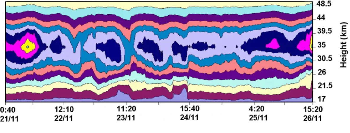
During the second campaign carried out in Puente del Inca, from 7–11 November 1994 a particular phenomenon was observed. In order to make evident this situation, a sim-ilar running mean process as Fig. 2 with a two hours box of the gained data was done (Fig. 3). This figure should be interpreted as a transversal cut of the stratosphere, in which can be clearly seen a wave structure that starts to shows up on 7 November

15

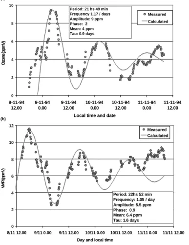
at about 18:00 Hs and its effect extends up to 10 November, depending on the strato-spheric layer. Figures 4a and b depict two particular layers at the 23.5 km and 30.5 km height, where we can observe the temporal variations of the ozone concentrations. It is clearly seen that on 8 November occurs the maximum of the perturbation, and from there on it attenuates gradually. In these pictures, a simulated damped sinus signal

20

was superposed to the measuring data with a best fit. This signal, represents the re-sponse of a second order damped system with a period of almost 22 h for the 23.5 km layer, with a maximum peak of more than 9 ppm and a minimum of about 1 ppm. It is interesting to note that the mean ozone VMR for 23.5 km is about 3 to 4 ppm. The time constant τ, i.e. when the wave peak drops down to 1/e of its maximum value, is about

25

0.9 days. If we analyze the 30.5 km layer we can find a wave period of 23 h approx-imately, with a maximum of almost 12 ppm and a minimum of somewhat higher than 2 ppm. The 35 km layer varies form 4 to 8 ppm. In other words, all layers experiment

ACPD

Full Screen / Esc

Print Version Interactive Discussion

c

EGS 2002 variations, which largely surpass their error bars. It is important to note that we have

tested the ozone data against the water vapor variation considering the 92 GHz water vapor measurements and the channel 0 of the ozone filterbank. We must recall the fact that the channel 0 is the farthest channel from the center frequency. This means that this channel is much more sensitive to atmospheric water vapor continuum than to

5

ozone. Both measurements had very similar water vapor values, and their variations did not present practically any correlation with the changes in the ozone concentra-tions. This is clear evidence that water vapor variations are not responsible for theses changes, but we may consider as a transport process or dynamic phenomenon that “modulates” the ozone concentration in the stratosphere. This may be caused by a

10

gravity wave produced in the troposphere due to airflow crossing The Andes Moun-tains, generally in the west-east direction. The Andes cordillera has a mean height of 5000 m, and a maximum of 7000 m and a width of approximately 150 km near Men-doza. It can be shown that if this vertical displacement of an air parcel is moved (under convective stability conditions) adiabatically and then liberated, this will oscillate from

15

its neutral flotation point with a frequency equal to the Brunt-V ¨ais ¨ala frequency (McIl-veen, 1992). This situation produces a wave train, which propagates upwards and horizontally producing quasi sinusoidal variations in the air density and pressure, car-rying moment and energy fluxes (Hocking, 1996; Brasseur and Solomon, 1986). Once the perturbation is originated, the amplitude of the wave starts to grow exponentially

20

as the air density decreases exponentially, assuming that there is no losses in energy as the wave propagates. Analogously, the wavelength of the gravity wave, in general, increases with height due to the air density decrease, and therefore the propagation velocity should be larger. It can be observed, in Fig. 3 that the amplitude of the waves increases up to a given height, and then, it starts to damp down. This seems to happen

25

starting about the 35 km layer.

According to the Argentine Weather Service, during the days 5, 6 and 7 November, the wind prevailed from the southeast and east sectors, with velocities of about 20 to 40 km/h in the Mendoza region and the sky was cloudless. The atmospheric pressure

ACPD

Full Screen / Esc

Print Version Interactive Discussion

c

EGS 2002 for Mendoza city in this period of time was: day 5 varied from 931 hPa (normal pressure

for Mendoza) to 923 hPa, day 6 between 936 and 933 hPa, day 7 the pressure was nor-mal. During day 8, the sky remained cloudless and the wind blew with normal velocity. The pressure fell down continuously reaching at the afternoon 927 hPa. During day 9, the wind prevailed from the south (presence of a dry south front) with velocities in

5

the morning of 35 km/h and decreasing towards the afternoon in 18 km/h. The atmo-spheric pressure oscillated between 930 and 934 hPa. Starting the afternoon of day 10, the sky presented some clouds and the wind direction was from the east. At day 11, arrived a fresh air mass from the south, increasing the cloudiness and decreasing markedly the temperature. The barometer indicated a strong fall in the pressure, going

10

down to 923 hPa. About the noon of that day the water vapor content reached values of about 2.5 g/cm2. Summarizing, the weather condition was, during practically all the week, very favorable for radiometric measurements.

The phase velocity of the gravity wave through the air will contribute positively or neg-atively to the wind velocity for a given height, depending on the sign of both velocities.

15

In the particular case of the stratosphere and mesosphere, the gravity waves could produce a positive or negative acceleration of the zonal wind, which changes its sign or sense of propagation seasonally, i.e. between winter and summer. The difference between the horizontal phase velocity and the wind mean velocity is named the intrin-sic phase velocity. In the case that the wave phase velocities and the zonal wind are

20

the same but with opposite signs, an standing wave will be produced, that could only be observed if several instruments are located along the air flow. It can be shown, that when both velocities tends to zero, the amplitudes of waves will grow enough to pro-duce the breaking of the wave. For a more detailed discussion see Hocking (1995) and Brasseur and Solomon (1986). Let us analyze, with more detail the layer of 23.5 km

25

height. The period of the wave is almost 22 h, or its frequency is 1.1 1/days. If we suppose that The Andes has a width of 150 km in the latitude of Puente del Inca, and a height around 7000 m. We can estimate the wavelength of the airflow passing through the mountains at 7000 m height in 300 km. Considering this 300 km as an estimation

ACPD

Full Screen / Esc

Print Version Interactive Discussion

c

EGS 2002 or the wavelength of the 23.5 km layer, we can calculate the intrinsic phase velocity

(mean zonal wind velocity – wave phase velocity) of the wave as:

v= λ × f = 300 × 103m × 1.1/86.400 s= 4 m/s (1)

In November, the zonal wind blows in the east-west direction, and if we consider an approximate zonal mean wind of 5 m/s we can calculate the horizontal wave phase

5

velocity as:

v= u − c (2)

where u is the mean zonal wind velocity, c is the wave phase velocity and v is the intrinsic velocity. Therefore, the phase velocity would be: c= 5 − 4 = 1 m/s.

4.2. Case 2: Variation of the ozone concentration during 23 August 1996 under Zonda

10

wind condition in Benegas, Mendoza

The Zonda wind, like the Chinook in USA or the F ¨ohn in the European Alps, is a very dry and hot wind which blows leeward with high intensity and whose effects normally extends up to hundred kilometers away from the mountains. The Zonda wind blows down on the eastern hillside of The Andes. This normally appears under the presence

15

of a low-pressure system in the south of Argentina and Chile and a high-pressure system at the east of Uruguay. The low-pressure system in the south provokes the entrance of a cold front, which arrives the Mendoza, and San Juan region some hours or days after the Zonda has been established. This phenomenon can be explained as an air flow which forcedly ascends in the Pacific Ocean, or in the western hillside of The

20

Andes, saturated adiabatically, and descending dry adiabatically on the eastern hillside of The Andes. In general, this meteorological phenomenon produces precipitation on the western hillside and snow in the peak of the mountains. But in the western side (Mendoza and San Juan region) the wind can provoke strong increases of the temperature of about 4◦C per each kilometer of mountain height.

ACPD

Full Screen / Esc

Print Version Interactive Discussion

c

EGS 2002 The meteorological situation of 23 August 1996, indicates clearly a classical structure

of Zonda, where at noon was already blowing in San Juan (north of Mendoza Province) at 40 km/h and in Malarg ¨ue (south of Mendoza Province) at 80 km/h. The atmospheric pressure can reach very low values such as 910 or 900 hPa, for Mendoza city (normal pressure is about 930 hPa). The Zonda blew in the surface from 15:00 until 04:00 of day

5

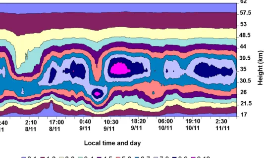
24. In that day the air dryness was practically absolute, and the temperature reached 34◦C (a very high value for that month). At 21:00 the Zonda wind was in its apogee blowing mostly in all Mendoza Province. “El Plumerillo” airport reports a temperature of 33◦C, a dew point of – 38◦C, and wind velocity of about 65 km/h In Fig. 5 we can see, in a similar way as it was done for case 1, a running mean with a box of two hours long

10

practiced on the radiometric data for different stratospheric layers. This integration time assures us a reasonable radiometric resolution for all layers. For the 37 km layer, we will have in the worst case, a measurement error of about 7% Thus the ozone VMR for this layer will yield 7 ± 0.50 ppm. In this particular case, the ozone concentration for this height varies, from 7 ppm down to values near 5 ppm. Whereas, for the 23.5 km layer,

15

the ozone VMR mean value (in normal conditions) is about 3.5 ± 0.3 ppm, considering a measurement error of 9%. This layer experiments variations in its concentration from 9 ppm to 5 ppm.

Within the measurement period the 23.5 km layer presents clearly a wave structure with a maximum occurring at 13:00 and with a minimum around the 20:30, which

per-20

mit us to estimate a wave period (considering a pure sinus) of about 14 h long. This phenomenon may be described as a gravity wave process promoted by the Zonda wind flowing across The Andes cordillera, in west-east direction. The zonal wind for this season of the year is west-east. Let us consider, like in the former case, and only to get an estimation, the same wavelength for the 23.5 km height. Using Eq. (1), the

25

intrinsic wave velocity would be about 6 m/s. Assuming a mean zonal wind velocity of 8 m/s in the west-east direction for that time of the year and taking into account Eq. (2), we can calculate the horizontal wave phase velocity, which yields in this case 2 m/s.

ACPD

Full Screen / Esc

Print Version Interactive Discussion

c

EGS 2002

5. Conclusions

The results show that in the average, the stratospheric ozone profiles has not under-gone a detectable and persistent reduction in time, within the uncertainty range of our instrument (measurement errors are from 2% to 11% of the volume mixing ratio according to the height and season of the year). However, the instrument is able to

5

detect variations with a minimal temporal resolution of an hour, and a spatial resolu-tion from 4 km to 5 km, particularly between 15 km and 45 km height. These observed variations are mainly due to dynamical processes associated to gravity waves, gener-ated by airflows over The Andes Mountains. These waves can promote a remarkable variation in the ozone concentrations for different layers, and may have periods, which

10

oscillates from 14 to 22 h, as are here reported.

Acknowledgements. The authors wish to thank the University of Mendoza, the

Max-Planck-Institut f ¨ur Aeronomie, and the Argentinean-German Scientific and Technological Cooperation, for their support to Project TROPWA.

References

15

Brasseur, G. and Solomon, S.: Aeronomy of the Middle Atmosphere, Second edition. Reidel Publishing Company, ISBN 90-277-2344-3, 1986.

Chandrasekhar, S.: Radiative Transfer, Dover Publications, Inc., New York, USA, 1960. Hocking, W. K.: Small-Scale Dynamics of the Upper Atmosphere: Experimental Studies of

Gravity Waves, in: the The Upper Atmosphere, (Eds) Dieminger, W., Hartmann, G. K., and 20

Leitinger, R., (Ed) Springer-Verlag Berlin Heidelberg New York, ISBN 3-540-57562-6, 1996. Keating, G., Pitts, M., and Young, D.: “Ozone reference models for the middle atmosphere”,

Adv. Space Res., 10, 12, 317–355, 1990.

McIlveen, R.: Fundamentals of weather and climate, (Ed) Chapman and Hall, London, SE1 8HN, 1992.

25

Puliafito, C., Puliafito, E., Hartmann, G., and Quero, J. L.: Determination of stratospheric ozone profiles and tropospheric water vapor content by means of microwave radiometry,

Proceed-ACPD

Full Screen / Esc

Print Version Interactive Discussion

c

EGS 2002

ings of the VIII Simp ´osio Brasileiro de Microondas e ´Optica (SBMO 98), Joinville – SC, Brasil, July 1998, pp. 274–278, 1998.

Puliafito, S. E., Bevilacqua, R., Olivero, J., and Degenhardt, W.: Retrieval error comparison for several inversion techniques used in limb-scannig millimeter wave spectroscopy, J. Geophys. Res., 100, D7, 14 257–14 268, 1995.

5

Remsberg, E., Russell, III, J. M., and Wu, C. Y.: An iterim reference model for the variability of the middle atmosphere water vapor distribution, Adv. Space Res., 10, 6, 51–64, 1990. Rodgers, C. D.: Characterization and error analyses of profiles retrieved from remote sounding

measurements, J. Geophys. Res., 95, 5587–5595, 1990.

Rodgers, C. D.: Retrieval of atmospheric temperature and composition from remote measure-10

ments of thermal radiation, Rev. Geophys., 14, 609–624, 1976.

Schlink, U., Puliafito, J. L., Herbarth, O., Puliafito, E., Richter, M., Puliafito, C., Rehwagen, M., Guerreiro, P., Quero, J. L., and Behler, J. C.: Ozone-Monitoring in Mendoza, Argentina: Initial Results, Air & Waste Management, ISSN 1047-3289, 49, 82–87, 1999.

Ulaby, F. T., Moore, R. K., and Fung, A. K.: Microwave remote sensing. Active and Passive, 15

ACPD

Full Screen / Esc

Print Version Interactive Discussion

c

EGS 2002

Figure 1. Seasonal stratospheric ozone mean values over Mendoza during the period 1993-2000

15 20 25 30 35 40 45 0 1 2 3 4 5 6 7 8 9 VMR (ppmV) Height (km) Summer Autum Winter Spring

ACPD

Full Screen / Esc

Print Version Interactive Discussion

c

EGS 2002

Figure 2. Stratospheric ozone variations (ppmV) over Puente del Inca (2700 m.a.N.s.l.) at the Andes Mountains from 21 to 26 November 1993. The data were integrated using a two hours running mean box

Fig. 2. Stratospheric ozone variations (ppmV) over Puente del Inca (2700 m.a.N.s.l.) at the

Andes Mountains from 21 to 26 November 1993. The data were integrated using a two hours running mean box.

ACPD

Full Screen / Esc

Print Version Interactive Discussion

c

EGS 2002 Figure 3. Similar running mean process as figure 2, but for ozone measurements

(ppmV) carried out in Puente del Inca from 7 to 11 November 1994. Large ozone variations can be observed compared to figure 2

Fig. 3. Similar running mean process as Fig. 2, but for ozone measurements (ppmV) carried

out in Puente del Inca from 7 to 11 November 1994. Large ozone variations can be observed compared to Fig. 2.

ACPD

Full Screen / Esc

Print Version Interactive Discussion

c

EGS 2002

Figure 4. Large ozone variations during November 1994 at Puente del Inca (see figure 3) for 23.5 km (a), and 30. 5 km layers (b). Circles represents the retrieved data and continuous line represents the adjusted damped sinus wave, which starts at day 8 and end at the beginning of day 11.

0 2 4 6 8 10 8-11-94 12.00 9-11-94 0.00 9-11-94 12.00 10-11-94 0.00 10-11-94 12.00 11-11-94 0.00 11-11-94 12.00 Local time and date

Ozone (ppmV) Measured Calculated Period: 21 hs 49 min Frequency 1.17 / days Amplitude: 9 ppm Phase: 2 Mean: 4 ppm Tau: 0.9 days (a) 0 2 4 6 8 10 12 8/11 12.00 9/11 0.00 9/11 12.00 10/11 0.00 10/11 12.00 11/11 0.00 11/11 12.00 Day and local time

VMR (ppmV) Measured Calculated Period: 22hs 52 min Frequency: 1.05 / day Amplitude: 5.5 ppm Phase: 0.9 Mean: 6.4 ppm Tau: 1.6 days (b)

Fig. 4. Large ozone variations during November 1994 at Puente del Inca (see Fig. 3) for 23.5 km (a), and 30.5 km layers (Circles represents the retrieved data and continuous line represents

ACPD

Full Screen / Esc

Print Version Interactive Discussion

c

EGS 2002 Figure 5. Stratospheric ozone variations for different layers at Benegas (850 m.a.N.s.l.), Mendoza, during Zonda wind event on 23 August 1996

0 2 4 6 8 10 12.53 13.23 13.53 18.02 18.33 19.02 19.42 20.13 21.06 Local time Ozone (ppmV) 19 23.5 28 32.5 37 41.5 46 50.5 Layers in km:

Fig. 5. Stratospheric ozone variations for different layers at Benegas (850 m.a.N.s.l.), Mendoza,