HAL Id: hal-00302300
https://hal.archives-ouvertes.fr/hal-00302300
Submitted on 25 Feb 2004
HAL is a multi-disciplinary open access
archive for the deposit and dissemination of
sci-entific research documents, whether they are
pub-lished or not. The documents may come from
teaching and research institutions in France or
abroad, or from public or private research centers.
L’archive ouverte pluridisciplinaire HAL, est
destinée au dépôt et à la diffusion de documents
scientifiques de niveau recherche, publiés ou non,
émanant des établissements d’enseignement et de
recherche français ou étrangers, des laboratoires
publics ou privés.
hemisphere blocking
M. Wei, J. S. Frederiksen
To cite this version:
M. Wei, J. S. Frederiksen. Error growth and dynamical vectors during southern hemisphere blocking.
Nonlinear Processes in Geophysics, European Geosciences Union (EGU), 2004, 11 (1), pp.99-118.
�hal-00302300�
SRef-ID: 1607-7946/npg/2004-11-99
Nonlinear Processes
in Geophysics
© European Geosciences Union 2004
Error growth and dynamical vectors during southern
hemisphere blocking
M. Wei1,2and J. S. Frederiksen3
1CSIRO Atmospheric Research, Australia
2NCEP Environmental Modeling Center, Maryland, USA 3CSIRO Atmospheric Research, Aspendale, VIC 3195, Australia
Received: 27 May 2002 – Revised: 3 September 2003 – Accepted: 17 November 2003 – Published: 25 February 2004
Abstract. The structural organization of initially random perturbations or “errors” evolving in a barotropic tangent lin-ear model with time-dependent basic states taken from ob-servations, is examined for cases of block development, mat-uration and decay in the Southern Hemisphere atmosphere during April, November and December 1989. We determine statistical results relating the structures of evolved errors to singular vectors (SVs), Lyapunov vectors (LVs) and finite-time normal modes (FTNMs). The statistics of 100 evolved error fields are studied for six day periods or longer and com-pared with the growth and structures of leading fast growing SVs, LVs and FTNMs. The SVs are studied in the kinetic en-ergy (KE), enstrophy (EN) and streamfunction (SF) norms, while all FTNMs and the first LV are norm independent. The mean of the largest pattern correlations between the 100 error fields and dynamical vectors, taken over the five fastest grow-ing SVs, in any of the three norms, or over the five fastest growing FTNMs, increases with increasing time interval to a value close to 0.6 after six days. Corresponding pattern cor-relations with the five fastest growing LVs are slightly lower. The leading dynamical vectors (SVs 1, FTNM1 or LV 1) gen-erally, but not always, give the largest pattern correlations with the error fields. It is found that viscosity slightly in-creases the average correlations between the evolved errors and LV 1 and evolved SVs 1. Mean pattern correlations with fast growing dynamical vectors increase further for time in-tervals longer than six days.
The properties of the dynamical vectors during Southern Hemisphere blocking are briefly outlined. After a few days integration, the structures of the leading evolved SVs in the KE, EN and SF norms, are in general quite similar and also similar to some of the dominant FTNMs that are norm in-dependent. For optimization times of six days or less, the evolved SVs and FTNMs are, in general, different from the dominant LVs on the same day. Nevertheless, amplification factors of the first FTNMs and first LVs are very similar, and also similar to, but slightly larger than, the mean
amplifica-Correspondence to: J. S. Frederiksen
(jorgen.frederiksen@csiro.au)
tion factor of 100 initially random perturbations in the SF norm, while the amplification factors in the SF norm of KE SVs 1 and SF SV 1 are much higher. For longer optimiza-tion times, the first SVs and the first FTNM increasingly turn towards the leading LV with convergence achieved within a month.
1 Introduction
In both the Southern and Northern Hemispheres, numeri-cal weather forecasts during the onset and decay of block-ing, frequently suffer from rapid loss of predictability (e.g. Tibaldi et al., 1995; Molteni et al., 1996). The inability of numerical forecast models to accurately predict blocking transitions is also a limiting factor in producing successful medium and extended range forecasts.
The variability of forecast skill is related to the instabil-ity of the large scale flow, to analysis errors and to model deficiencies in physical processes, resolution and sub-grid scale parameterizations (Frederiksen and Davies, 1997 and references therein). In this study, we focus on error growth and predictability associated with initial condition errors and with instability processes of the large scale flow. Because of the uncertainty in the atmospheric basic state, weather forecasting should be formulated as a problem of predict-ing the probability density function of states in phase space or equivalently the infinite hierarchy of cumulants. For ex-ample, Leith (1974) used a second order closure model for two-dimensional turbulence to study the evolution of error spectra and their convergence towards an atmospheric type spectrum. Second order closure models have primarily been applied to the idealized problems of isotropic, and occasion-ally homogeneous, turbulence with zero mean fields (Fred-eriksen and Davies, 1997). Recently, tractable closures have been formulated for general inhomogeneous barotropic flows over topography incorporating prognostic equations for the mean fields and covariance and response function matrices (Frederiksen, 1999). However, for the multi-level primitive equation models used in numerical weather prediction the
only currently feasible way of predicting the statistics of fu-ture atmosphere states is through ensemble forecasting tech-niques which sample the possible initial conditions. Unfor-tunately, the covariance matrix of analysis error is poorly known.
It is generally agreed that the sample of initial conditions should include the rapidly expanding directions in phase space, but there is controversy over how the directions should be characterized (Toth and Kalnay, 1993, 1997; Houtekamer and Derome, 1995; Molteni et al., 1996; Anderson, 1996; Frederiksen, 1997; Szunyogh et al., 1997; Palmer et al., 1998). This is related to the question of whether atmospheric disturbances and errors are seen to develop essentially as ex-ponentially growing modes (Frederiksen, 1983; Simmons et al., 1983) or whether interference effect, leading to periods of super-exponential growth, are in general important (Far-rell, 1989; Schubert and Suarez, 1989; Frederiksen and Bell, 1990; Molteni and Palmer, 1993; de Pondeca et al., 1998a, b; Frederiksen and Branstator, 2001). As a consequence, a number of different methods of choosing ensemble perturba-tions to perturb the control initial condiperturba-tions have been pro-posed and implemented.
Rotated singular vectors in the total energy norm are used as ensemble perturbations at the European Centre for Medium Range Weather Forecasts (ECMWF) (Buizza and Palmer, 1995; Molteni et al., 1996; Palmer et al., 1998), while bred perturbations, which have been linked to Lya-punov vectors, are used at the National Centers for Envi-ronmental Prediction (NCEP) (Toth and Kalnay, 1993, 1997; Kalnay et al., 2002; Kalnay 2003). Recently Corazza et al. (2003) pointed out that bred vectors can efficiently repre-sent the background errors that dominate the analysis “errors of the day”. Houtekamer et al. (1996) use multiple analy-sis cycles to form their ensemble perturbations. It has also been suggested (Frederiksen and Bell, 1990) that superpo-sitions of fast growing normal modes would approximately characterize the instability and error growth in atmospheric flows over several days. An ensemble prediction scheme based on normal modes was successfully employed by An-derson (1996) for a low order dynamical system. Frederik-sen (1997) suggested that the important directions for er-ror growth are spanned by the dominant finite-time normal modes (FTNMs), the norm-independent eigenvectors of the tangent linear propagator.
Many insights into the roles of dynamical vectors in at-mospheric predictability have come from studies employing low order models (Lorenz, 1965; Trevisan, 1993; Ander-son, 1996), barotropic models (Frederiksen and Bell, 1990; Molteni and Palmer, 1993) and simplified and low verti-cal resolution baroclinic models (Farrell, 1989; Frederik-sen and Bell, 1990; Molteni and Palmer, 1993; Houtekamer and Derome, 1995). In our present study, partly for sim-plicity and partly because of our need to perform large en-sembles of simulations, we employ a barotropic model. We examine perturbation or “error” growth during the periods of block formation, maturation and decay in the Southern Hemisphere in April, November and December 1989.
Dy-namical processes during blocking may have a baroclinic component, particularly in the early stages of development (Frederiksen, 1983; Buizza and Molteni, 1996; de Pondeca et al., 1998a, b) and this may be reflected in error structures (Frederiksen and Bell, 1990). However, a large component of large scale error growth can be described by barotropic dy-namics particularly during the more mature phase of block-ing (Veyre, 1991; Frederiksen, 1998).
Ensemble prediction methods based on both SVs and bred perturbations, which have been linked to LVs, result in im-proved forecasts. However, much work still needs to be done to understand the relative effectiveness of ensemble forecast-ing systems based on different dynamical vectors. We need to improve our understanding of how errors become orga-nized as they grow and how their structures are related to dominant FTNMs, LVs and SVs in different norms. The main aim of this paper is to determine statistical relationships between the structures of evolving, initially random, errors and all these dynamical vectors during Southern Hemisphere blocking; a topic which to our knowledge has not previously been examined. We also briefly consider the properties, par-ticularly growth rates and structures, of the different dynam-ical vectors and the relationships between them. Southern Hemisphere blocks may have smaller scales, less rapid de-velopment, reach smaller amplitude and persist for shorter duration than Northern Hemisphere blocks. There is thus the possibility that these differences could alter the growth rates, convergence rates and scales of the blocking dynami-cal vectors in the two hemispheres, just as the sdynami-cales of SVs associated with Northern Hemisphere cyclogenesis (Palmer et al., 1998) and Northern Hemisphere blocking (Frederik-sen, 1997) differ considerably.
The plan of the paper is as follows. Section 2 summarizes the barotropic tangent linear equations for error growth and defines the propagator that maps an initial perturbation into an evolved field. Here we also define FTNMs, SVs and LVs and summarize some of their intrinsic properties. Section 3 contains a brief description of the synoptic situation during the Southern Hemisphere blocking events in April, Novem-ber and DecemNovem-ber 1989. It also describes the construction of the time-dependent basic states obtained from daily observed 300-mb streamfunction fields through linear interpolation. In Sect. 4, we examine the properties of LVs, SVs and FTNMs for Southern Hemisphere flows and for periods ranging from one day to one month in April; we study the norm depen-dence of SVs and compare them with FTNMs, which are norm independent, and with LVs.
In Sect. 5, we examine the structural organization of ini-tially random errors in April and relate their amplifications and evolved structures to dominant evolved SVs, LVs and FTNMs. Statistical results on pattern correlations between 100 evolved errors and SVs, LVs and FTNMs are displayed for periods out to six days. We also briefly mention the corre-sponding results for December. Section 6 contains a similar study for periods out to six days in November and as well for longer periods out to fourteen days. Our conclusions are presented in Sect. 7.
2 Theory and model details 2.1 Model formulation
We base our studies on the barotropic tangent linear equa-tions, for the reasons outlined in the Introduction. For flow on a sphere, the nondimensional form of the tangent linear vorticity equation is given by
∂ζ ∂t=−J (ψ, ¯ζ +2µ)−J ( ¯ψ , ζ )−ηζ −η 0∇4ζ, (1) where J (ψ, ζ )=∂ψ∂λ∂µ∂ζ−∂ψ ∂µ ∂ζ
∂λ, ψ is the streamfunction
per-turbation, ζ =∇2ψis the vorticity perturbation, while ¯ζ and
¯
ψ are the basic state vorticity and streamfunction respec-tively. The other parameters in Eq. (1) are as follows: t is time, λ is longitude, µ is sine of latitude, and η and η0 are the coefficients of viscosity representing drag and diffusion. All the variables are nondimensional with space coordinates scaled by the earth’s radius and time scaled by −1, the in-verse of the earth’s angular velocity.
The results reported here will depend to some extent on the choice of the viscosity used. Therefore, we examine ini-tially both the inviscid case and a case with a typical mag-nitude of the viscosity, so that comparison of the respective results gives an indication of their sensitivity to dissipation. In the viscous case, the coefficients of viscosity are chosen as
η=8.4×10⁻⁷s−1 and η0=2.5×10¹⁶m4/s. The spectral
ver-sion of the barotropic tangent linear equation is obtained by expanding the streamfunction and vorticity in spherical har-monics. We use a rhomboidal R15 truncation. The tangent linear spectral equations can then be written in the form
dx(t)
dt =M(t)x(t), (2)
where x=(. . . , Re(ζml), . . ., I m(ζml), . . .)T is the column
vector of the real and imaginary parts of vorticity spectral coefficients ζml, and M(t ) is the tangent linear operator
eval-uated on the observed basic state trajectory. The solution to Eq. (2) is
x(t)=G(t, t0)x(t0), (3)
where G(t, t0)is called the propagator. The tangent linear
equations are solved with a half-hour time step, which en-sures numerical stability and the basic states are determined as described in Sect. 3.
2.2 Finite-time normal modes
The eigenvectors of the propagator G(t, t0) are the
natu-ral genenatu-ralizations of normal modes to the case of time-dependent instability matrices, M(t ). The propagator sat-isfies an eigenvalue equation
[λνI − G(t, t0)]φν =0, ν =1, . . . , n, (4)
where λν=λν[t, t0]and φν=φν[t, t0]are the eigenvalues and
eigenvectors, and I is the unit matrix. The eigenvectors are
called finite-time normal modes (FTNMs) following Fred-eriksen (1997). The FTNMs have been obtained directly from the tangent linear model using a variant of Arnoldi it-erative methods (Arnoldi, 1951) and checked against results using the standard quotient reduction method and the ma-trix form of the propagator (Frederiksen, 1997). Since the Arnoldi method does not need the adjoint model for back-ward integrations, the computing cost for solving FTNMs is about half of that for SVs if the same model is used.
2.3 Singular vectors
Singular vectors (also known as optimal perturbations) have been extensively used for ensemble predictions at several nu-merical weather prediction centers, especially at ECMWF (Buizza and Palmer, 1995; Farrell and Ioannou, 1996; Szun-yogh et al., 1997; Palmer et al., 1998; Kalnay, 2003 and ref-erences therein). For the Euclidean inner product <x; y >, the norm of the perturbation at time t is given by
||x(t)||2=<x(t); x(t)>
=<G†(t, t0)G(t, t0)x(t0); x(t0)>, (5)
where G†(t, t0)denotes adjoint operator or Hermitian
conju-gate matrix with respect to the Euclidean inner product. It is obvious that the operator G†(t, t
0)G(t, t0)is symmetric, thus
its eigenvectors vν (ν=1, 2, . . . , n) can be chosen to form a
complete orthonormal basis in the n-dimensional space of linear perturbations. The eigenvalue-eigenvector equation
G†(t, t0)G(t, t0)vν =(σν)2vν (6)
has real eigenvalues (σν)2≥0 (Golub and Van Loan, 1996). The v-SVs, vν, evolve to the u-SVs, and σνuν=G(t, t
0)vν,
uνin turn are the eigenvectors of G(t, t
0)G†(t, t0); that is
G(t, t0)G†(t, t0)uν =(σν)2uν. (7)
The σν are termed the singular values of G(t, t0)and the
v-SVs and u-v-SVs are also called right singular vectors and left singular vectors respectively (Golub and Van Loan, 1996). When the dimension of G(t, t0)is not too large, the
singu-lar values σν, v-SVs and u-SVs can be calculated through a
singular value decomposition (Golub and Van Loan, 1996). Our tangent linear equations are formulated in terms of the vorticity spectral coefficients. Consequently, our norm squared is equal to the enstrophy (suitably normalized); we loosely refer to this norm as the enstrophy norm (EN). We shall also need to consider SVs in the streamfunction norm (SF) and in kinetic energy norm (for which the norm squared is equal to the kinetic energy). SVs in these norms can be obtained from the propagator formulated for the EN norm by a transformation of variables y(t )=Cx(t ) where C is a diagonal transformation matrix that depends only on the total wave number l. The SVs in these three norms will be referred to as EN SVs, SF SVs and KE SVs.
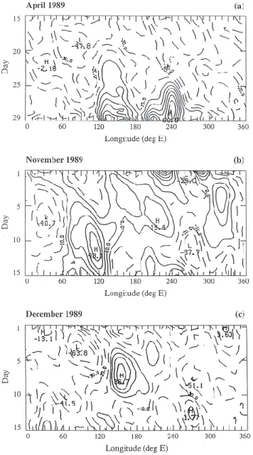
Fig. 1. Hovmoeller diagrams of blocking indices in 1989 in the
Southern Hemisphere for (a) the second half of April, (b) the first half of November, (c) the first half of December.
2.4 Lyapunov vectors and local Lyapunov exponents
In recent years, Lyapunov techniques have been employed in meteorology (Toth and Kalnay 1993; Palmer et al., 1998; Farrell and Ioannou 1996; Legras and Vautard 1996; Szun-yogh et al., 1997; Vannitsem and Nicolis 1997; Reynolds and Errico 1998; Corazza et al., 2003; Kalnay et al., 2002; Kalnay 2003), particularly in predictability and ensemble prediction studies. In this subsection, we summarize some of the properties of Lyapunov theory and define local Lyapunov exponents and Lyapunov vectors. As discussed in some of the above references, Lyapunov exponents (LEs) are global quantities, which only measure the long-time average expo-nential growth rates along different directions in the phase space. However, for meteorological and climate applications
the local and finite-time growth rates are usually more rele-vant. We define the finite-time Lyapunov exponents as
Lν(t2, t1) = 1 t2−t1 ln||x ν(t 2)|| ||xν(t 1)|| , (8)
where xν(t ) ∈ Fν(t ), Fν(t )are the set of disjoint subspaces
defined in papers such as Vastano and Moser (1991), Legras and Vautard (1996), and t2−t1=J 1t(J is a positive integer,
1t is the integration time step). Here, xν(t )is a vector of given magnitude in the direction of Fν(t ). Also || · || repre-sents the Euclidean norm. Clearly Lν(t2, t1)depend on t1, t2
and the position on the trajectory; they measure the average perturbation growth over the interval t2−t1. The global LEs
are recovered by taking the limit t2→∞. When J =1, they
are called local Lyapunov exponents in this paper, and they are denoted by Lν(t ). That is
Lν(t ) = 1 1t ln
||xν(t + 1t )||
||xν(t )|| . (9)
Both Fν(t )and Lν(t )are local properties of the dynamical system. They give the directions of perturbation growth and the growth rates in those directions. They can be used to identify the local instabilities of a dynamical system but it should be noted that they are, in general, different from the eigenvectors and eigenvalues of the stability matrix M(t ) at time t (the normal modes and their growth rates).
The algorithm we will use for computing the Lν(t )and
Fν(t )is based on the so-called standard method (Shimada and Nagashima, 1979; Benetin et al., 1980). The standard method consists of evolving a set of orthonormal vectors, chosen initially at random in the tangent space Tn(t )at X(t ), by integrating the equations for both the basic state flow which is taken from 300-mb streamfunction fields and the perturbations (2) or (3). The method determines the growth rates Lν(t ) and the associated Fν(t ). The Fν(t )
compo-nents of a perturbation will grow or shrink exponentially with
Lν(t ).
Since L1 is the largest growth rate, almost all uncon-strained perturbations will ultimately tend towards F1, the most unstable direction associated with the largest LE. This would mean, however, that only the leading Lyapunov vec-tor would be generated . To prevent this, it is necessary to ensure that the set of perturbations are orthogonal so that one member of the set approaches F1 and the others ap-proach Fν, ν=2, 3, . . ., n. To ensure this, it is necessary
to perform a Gram-Schmidt re-orthogonalization from time to time. In practice, we always carry out a modified Gram-Schmidt orthogonalization, which involves a double re-orthogonalization at each step. The set of orthonormal vec-tors obtained in this way characterizes the local directions of stretching or contraction of any perturbation and is iden-tical to the set obtained by orthogonalizing the Fν starting from F1(Vastano and Moser, 1991). We call this orthonor-mal set of vectors generated through the standard method Lyapunov vectors (LVs). Similar definitions of local Lya-punov exponents and LVs have been used by other authors
in meteorology (Legras and Vautard, 1996; Szunyogh et al., 1997; Vannitsem and Nicolis, 1997; Wei, 2000).
Finally, we must emphasize that all the LVs are local. The long-time average growth rates are given by corresponding global LEs, which are ordered from largest to smallest, so
L1≥L2≥. . . ≥Ln, and their local growth rates are described respectively by the local LEs L1(t ), L2(t ), . . . , Ln(t ). How-ever, at any time t, the local growth rate of LV 1 is not always largest, although its long-time average growth rate (L1) is the largest. The LV at a time t with largest local Lyapunov exponent (Lν(t ), where ν is not necessarily equal to 1) has maximum local growth rate, and will be referred to as MLV 1 at this time. Similarly, the LV with the second largest local growth rate will be referred to as MLV 2 and so on.
3 Synoptic situations and observed basic states
Blocking highs derive their name from the fact that they are quasi-stationary features that tend to occur in preferred ge-ographical locations and block, or deflect towards the pole, the normal eastward progression of weather systems. During their growth and decay they tend to be associated with a loss of predictability.
In this study we examine error growth associated with de-veloping blocks that formed in the regions of Australia-New Zealand or in the Central Pacific in April, November and De-cember 1989. As noted in a number of observational studies (e.g. Lejenas, 1984) the Australian-New-Zealand region is the primary preferred region for blocking action in the South-ern Hemisphere. The blocking indices for these three months are shown in Fig. 1. The daily Hovmoeller diagrams for the second half of April and the first halves of November and December are shown in Figs. 1a–c respectively. These in-dices are based on observations and taken from the Climate Monitoring Bulletin of the Australian Bureau of Meteorol-ogy (CMB, 1989). Their definition of the blocking index (BI) for the Southern Hemisphere is as follows:
BI =0.5 (U25S+U30S +U55S+U60S
−U40S−U50S−2U45S), (10)
where U denotes the 500 mb zonal wind at the latitudes indi-cated by subscripts. This definition ensures a positive block-ing index for blockblock-ing highs in southern latitudes and for dipole high-low structures with the highs to the south of the lows, and vice versa for negative blocking index.
During late April, blocking high-low dipoles formed at the longitudes of eastern Australia and in the central Pacific. These events are associated with positive blocking indices around 150 east and 240 east longitude between 24 April and the end of the month (Fig. 1a). The eastern Australian block was preceded by a large amplitude trough that devel-oped to the southwest of Western Australia around 20 April. This blocking dipole caused a splitting of the jet stream into two distinct currents as it amplified. This is seen in Fig. 2a, which shows the streamfunction for the flow at 300 mb at
00:00 UTC on 24 April. The blocking dipole is equiva-lent barotropic and, as usual, is more evident at lower lev-els (not shown). By 26 April the block had moved down-stream to a location near New Zealand and started to decay. This was also the time when the central Pacific block began its development near 240 east longitude. These events are seen in Fig. 2b, which shows the 300 mb streamfunction at 00:00 UTC on 26 April.
For April (also for November and December) we shall fo-cus on barotropic processes associated with 300 mb basic states, which is why we have concentrated on this level in the above discussion even though the blocks are more evi-dent at lower levels. The reasons for choosing the 300 mb level for analysing barotropic processes relate to theoretical arguments that show that a higher level than the traditional 500 mb one is appropriate for barotropic model studies (Sim-mons et al., 1983).
During November 1989, blocking activity was above av-erage from east of 0 degrees longitude to the central Pa-cific. Our interest is focussed on the blocking dipole that formed early in the month near 120 east longitude,as shown by the blocking index in Fig. 1b. The block started devel-oping around 8 November and a blocking dipole pattern ex-tending through the troposphere became established over In-dian Ocean on about 11 November. As a consequence, the jet stream was split into two quite distinct branches across the Indian Ocean, as seen at 00:00 UTC on 12 November in Fig. 2c, which shows the 300 mb streamfunction. Towards the middle of the month, the block moved downstream and decayed.
In early December, a blocking high pressure system be-gan developing over the southern most extent of the Tasman sea between Australia and New Zealand. The corresponding positive blocking index near 150 east longitude is shown in Fig. 1c. By 00:00 UTC on 9 December a large amplitude blocking dipole extended through the troposphere as shown in the 300 mb streamfunction field in Fig. 2d. The block sub-sequently decayed after 10 December.
As is common practice in mechanistic studies such as this one (e.g. Buizza and Molteni, 1996; Frederiksen, 2000 and references therein), our basic states are constructed from ob-served daily 300 mb streamfunction fields at 00:00 UTC dur-ing the three periods discussed above. We linearly interpo-late to obtain the time-dependent fields needed every half hour in simulations and theoretical studies. We have also performed some comparisons using twice-daily data to estab-lish the generality after findings. Because our basic states are constructed from observations, they include all effects acting on the atmosphere including diabatic heating, baroclinic and topographic effects. For these basic states to be solutions of the nonlinear barotropic vorticity equations additional time-dependent forcing (that may be calculated as a residual) must be included to compensate for neglected physical processes.
Fig. 2. The basic state streamfunction (in km2/s) at 300 mb on (a) 24 April, (b) 26 April, (c) 12 November, (d) 9 December 1989.
4 SVs, LVs and FTNMs in April
Here, we compare the properties and evolutions of SVs, LVs and FTNMs during periods between 20 April to 26 April. We calculate the SVs in three different norms, i.e. KE SVs, SF SVs and EN SVs. In contrast, all the FTNMs are norm independent as is the first Lyapunov vector.
Figure 3 shows SVs in each of the three norms for the optimization period between 20 and 26 April and in the in-viscid case. The structures for the viscous case are very sim-ilar. The initial v-SVs are depicted on 20 April (Figs. 3a, b and c) and the evolved or u-SVs are shown on 26 April
(Figs. 3d, e and f). The v-SVs depend sensitively on norm, with the EN norm characterized by large-scale disturbances with large zonal flow contributions, the KE norm yielding in-termediate scale disturbances, and the SF norm giving initial small-scale disturbances. In general, the v-SVs associated with blocking show more variations in scale in the different norms than v-SVs associated with cyclogenesis (Palmer et al., 1998). In contrast to the sensitive norm dependence of the v-SVs, the evolved SVs on 26 April are much more sim-ilar in their structures (Figs. 3d, e and f). They are also quite similar to the structure of FTNM 1 for the period from 20 to 26 April shown in Fig. 4a for the inviscid case. Note that the
Fig. 3. The streamfunctions of initial and evolved SVs 1 during the period between 20 to 26 April 1989 in the inviscid case. Shown are the
u-SVs shown in Figs. 3d, e and f are scaled to have similar
amplitudes to FTNM 1 displayed in Fig. 4a for comparison. The corresponding v-SVs in Figs. 3a, b and c are also scaled by the respective scaling factors.
Quantitative results regarding the similarity of final SVs and FTNM 1 are given in Fig. 5a, which shows the pattern correlations between SV 1 in each norm and FTNM 1 for periods starting on 20 April and finishing on subsequent suc-cessive days to 26 April. Here the pattern correlation is de-fined as follows. We define the inner product of any two real Southern Hemisphere physical space streamfunction fields
X(λ, µ, t )and Y (λ, µ, t ) at time t by {Y (λ, µ, t ), X(λ, µ, t )} = 1 2π 2π Z 0 dλ 0 Z −1 dµY (λ, µ, t )X(λ, µ, t ), (11)
where λ is longitude and µ is sin(latitude). Then the pattern correlation between X and Y is defined by
Ac=
{Y, X} {Y, Y }12{X, X}12
. (12)
We note that the sign of SVs is arbitrary while the structures of FTNMs may depend on their particular phase. As a con-sequence, the pattern correlations shown are the largest taken over all phases of the FTNMs.
From Fig. 5a, we see that there is a general tendency for the pattern correlations between the SVs 1 in each norm and FTNM 1 to increase with increasing time period, particularly at and beyond three days. The pattern correlations are partic-ularly high for the periods ending on 24 and 26 April when the respective eastern Australian and central Pacific blocks are amplifying.
By 26 April, the evolved SVs 1 in Figs. 3d, e and f and FTNM 1 have dipole or multi-pole structures, of similar scales to the central Pacific block, which are focussed in the blocking region near 120◦W. In fact, similar evolved SV structures are obtained for shorter optimization times end-ing on 26 April. In Figs. 4b and c we show the initial v-SV 1 on 23 April and the final evolved v-SV 1 on 26 April in the KE norm and for the optimization period between 23 and 26 April. The centre of action of the initial v-SV 1 on 23 April is now located in the sector between 120◦E and 180◦E near 60◦S; this is to be compared with the initial v-SV 1 on 20 April (Fig. 3b), which also has a number of strong centres located upstream of this region. The evolved SVs 1 on 26 April are, however, much more similar (Figs. 3e and 4c), particularly in the sector between 0 and 120◦W. Again both the initial and evolved and SVs shown in Figs. 4b and 4c are properly scaled.
Next, we examine the structures of dominant LVs in late April, again for the inviscid case. Figures 4d and 4e show the structures of the leading LV on 24 and 26 April respec-tively. The leading LV is a local property of the system, it depends on time, and is associated with the largest global Lyapunov exponent. That is, over a sufficiently long period
Table 1. Nondimensional amplification factors of five fastest
grow-ing of FTNMs and LVs, sgrow-ingular values of EN SVs, KE SVs and SF SVs for period from 23 to 26 April 1989 in the inviscid case.
Index 1 2 3 4 5 |λν| 2.093 2.091 2.083 2.057 1.852 Lν 2.278 1.678 2.258 1.978 1.695 σENν 27.119 17.028 12.449 11.037 10.633 σKEν 11.516 8.144 7.667 6.700 6.389 σSFν 17.594 14.071 13.728 12.419 11.142
of time it will have the largest average growth rate of all the Lyapunov vectors. However, its growth rate at a given time may be exceeded by a sub-dominant LV. We define the max-imum growth Lyapunov vector 1 (MLV 1) as the Lyapunov vector which, at a given time, has the largest local exponent or growth rate. On 24 April, LV 1 is in fact also MLV 1. However on 26 April a sub-dominant LV has the largest lo-cal growth rate. The MLV 1 on 26 April is shown in Fig. 4f. All the LVs 1 and MLV 1 shown in Figs. 4d-4f are properly scaled to compare with the evolved SVs 1 on 26 April. These Lyapunov vectors have been obtained by starting with ran-dom initial perturbations on 26 March 1989, integrating the tangent linear model forward and using the standard method (Shimada and Nagashima, 1979; Benetin et al., 1980) to ob-tain the left LVs and global Lyapunov exponents. In princi-ple, the integration should start from −∞, but in practice a month is sufficient time. This has been established by com-paring results obtained using different initial starting points and different initial random perturbations.
Both LV 1 and MLV 1 on 26 April have significant am-plitude in the blocking region between 60◦W and 120◦W; however, they also have a number of significant centres out-side this region. On the whole, they appear to be less similar in structure to the evolved SVs 1 in Figs. 3d, e and f than are the evolved SVs 1 to each other and to FTNM 1. This is con-firmed by calculating the pattern correlations between LV1 and the evolved SVs 1 and FTNM 1. Figure 5b shows these pattern correlations for LV 1, on successive days between 21 and 26 April, and evolved SVs 1 and FTNM 1 for peri-ods starting on 20 April and finishing on successive days to 26 April. We note from Fig. 5b that all but one of the shown pattern correlations are less than 0.4 and generally consider-ably less than between evolved SVs 1 and FTNM 1 (Fig. 5a), particularly on 24 and 26 April. To some extent these results might be expected, since the time intervals (up to six days) are not long enough for the evolved SVs 1 and FTNM 1 to converge to LV 1.
We now turn to a consideration of the amplification factors of SVs, LVs and FTNMs. We define the amplification factor
Fig. 4. The streamfunctions of dominant dynamical vectors during the period between 20 to 26 April 1989 in the inviscid case. Shown are (a) FTNM 1 during 20 to 26 April, (b) The initial KE SV 1 for 23 to 26 April, (c) the evolved KE SV 1 for 23 to 26 April, (d) LV 1 on
20 21 22 23 24 25 26 27 April 0.0 0.2 0.4 0.6 0.8 1.0 correlation
EN SV 1
KE SV 1
SF SV 1
a
20 21 22 23 24 25 26 27 April 0.0 0.2 0.4 0.6 0.8 1.0 correlationEN SV 1
KE SV 1
SF SV 1
FTNM 1
b
20 21 22 23 24 25 26 27 April 0 2 4 6 8 10 12 14 amplificationFTNM 1
LV 1
mean
EN SV 1
0.2*KE SV 1
0.2*SF SV 1
c
20 21 22 23 24 25 26 27 April (viscous) 0 1 2 3 4 5 6 7 amplificationFTNM 1
LV 1
mean
EN SV 1
0.2*KE SV 1
0.2*SF SV 1
d
20 21 22 23 24 25 26 27 April 0 20 40 60 80 100 120 singular valueEN SV 1
KE SV 1
SF SV 1
e
20 21 22 23 24 25 26 27 April (viscous) 0 10 20 30 40 50 60 singular valueEN SV 1
KE SV 1
SF SV 1
f
Fig. 5. The pattern correlations and amplification factors of dominant dynamical vectors in both inviscid and viscous cases during periods
from 20 to 21, 22, . . ., 26 April 1989. Shown are (a) pattern correlations of FTNMs 1 with the evolved EN SVs 1 (3), KE SVs 1 (4) and SF SVs 1 (2) in the inviscid case, (b) pattern correlations of LVs 1 on 21, 22 . . ., 26 April with the evolved EN SVs 1 (3) , KE SVs 1 (4), SF SVs 1 (2) and FTNM 1 (∗) in the inviscid case, (c) amplification factors of FTNM 1 (∗) and LV 1 (+), amplification factors in SF norm of EN SV 1, KE SV 1 (scaled by 0.2), SF SV 1 (scaled by 0.2) and the mean of 100 evolved errors (thick solid line) and mean ± standard deviation of 100 evolved errors (thick dashed lines) in the inviscid case. Also shown in (d) are results as in (c) but with viscosity, (e) singular values of EN SV 1 (3), KE SV 1 (4), SF SV 1(2)in the inviscid case and (f) as in (e) but with viscosity.
for a perturbation field X(λ, µ, t) between t0and t as Af(t, t0) = {X(λ, µ, t ), X(λ, µ, t )}12 {X(λ, µ, t0), X(λ, µ, t0)} 1 2 , (13)
where the inner product is defined in Eq. (11). One can choose different types of fields X(λ, µ, t) (for example, streamfunction or vorticity) such that Af(t, t0)represents the
amplification factors in different norms. In this study, we have used EN, KE and SF norms. Both FTNM 1 and LV 1 are norm independent. For SVs, σ1 in each of these three
norms represents the amplification factor of SV 1 over the same period of time in the chosen norm.
In order to compare the growth of singular vectors associ-ated with different norms and initially random perturbations, it is necessary to choose a common norm which we choose to be the SF norm. In the SF norm, Figs. 5c and d show the amplification factors between 20 and 26 April for FTNM 1, LV 1, EN SV 1, KE SV 1 and SF SV 1 in the inviscid and viscous case respectively. Figures 5e and f give the cor-responding singular values for SVs 1 in each of the three norms in the inviscid and viscous cases respectively. These singular values are also the amplification factors of SVs 1 in the respective norms. We note that the amplification fac-tors of FTNMs are just the magnitude of the corresponding eigenvalues |λν|. The amplification factors of LVs 1 from 20 April to successive days have been calculated from the lo-cal Lyapunov exponents during these periods. Also shown in Figs. 5c and d are the mean and mean ± standard deviation of 100 amplification factors of 100 initial randomly gener-ated error fields in SF norm in thick solid and thick dashed lines respectively.
The initial random perturbations are chosen from a Gaus-sian distribution in which the magnitudes of the streamfunc-tion spectral coefficients are proporstreamfunc-tional to (2l + 1)−1; that is, |ψml|∼2l+11 . This means that
P
m|ψml|is exactly
con-stant in the inner rhomboid where l ≤ R and falls off with total wave number in the outer rhomboid. It also means that the total wave number spectrum of kinetic en-ergy, e(l)=P
ml(l+1)ψmlψml∗ , increases linearly in the
in-ner rhomboid and falls off with wave number in the outer rhomboid. There are uncertainties in the determination of the analysis error covariance matrix. However, the linear increase of the total wave number spectrum of kinetic en-ergy in the inner rhomboid to l=R=15 and fall off in the outer rhomboid appears to be consistent with typical esti-mates of 2-day forecast errors as seen in Fig. 4d Molteni et al. (1996); their spectrum for differences between ECMWF and Deutsche Wetterdienst analyses is however flatter.
Figures 5c and d show that FTNM 1 and LV 1 have very similar amplification factors in late April although, as we have noted, there are significant structural differences be-tween FTNM 1 and LV 1 during this period. Now, suppose that there is a perturbation whose local growth rate is always the same as the largest local Lyapunov exponent during the period from 20 to 26 April; that is, this perturbation is MLV 1 at each time. Then the amplification factors of this
pertur-Table 2. As in pertur-Table 1 but for period from 20 to 26 April.
Index 1 2 3 4 5 |λν| 8.156 5.576 4.261 3.877 3.789 Lν 7.282 3.263 4.605 4.002 5.538 σENν 103.653 63.495 46.177 38.229 33.794 σKEν 44.517 41.801 33.037 24.524 23.562 σSFν 77.457 71.407 54.724 40.771 37.997
bation are slightly larger than those of LV 1 (not shown). We also note from Figs. 5c and d that FTNM 1 and LV 1 have similar, but slightly larger, amplification factors than the mean amplification factor of the 100 initially random er-rors in the SF norm. Also in the SF norm, the amplification factors of KE SV 1 and SF SV 1 are much larger than for LV 1 and FTNM 1 after a few days. After about three days the amplification factors of KE SV 1 and SF SV 1 are about an order of magnitude or more larger than the mean ampli-fication factor of 100 initially random errors. However, in the SF norm, the amplification factors of EN SV 1 are lower than the mean amplification factor of 100 initially random errors in either the inviscid or viscous case (Figs. 5c and d), although the EN SV 1 has even larger amplification factors in the EN norm than KE SV 1 and SF SV 1 in their respec-tive norms (Figs. 5e and f). As expected, in both inviscid and viscous cases, the amplification factors of SVs 1 in their re-spective norms are much larger than those of FTNM 1 and LV 1 as shown in Figs. 5e and f.
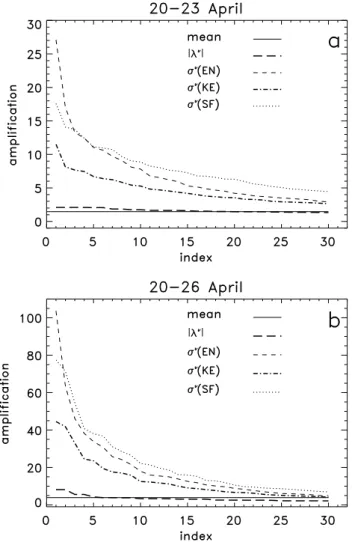
In the above figures, we have shown the amplification fac-tors of KE SV 1, SF SV 1, EN SV 1, FTNM 1 and LV 1. For the inviscid case, the amplification factors of the five fastest growing FTNMs and top five LVs for the three-day period (20 to 23 April) and six-day period (20 to 26 April) are shown in Tables 1 and 2, respectively. Also shown are the top five singular values in EN, KE and SF norms. As expected the amplification factors for each type of dynamical vector in the respective norms are larger for the longer periods. We also note the singular values of SVs fall off more rapidly with in-creasing index than they do for LVs and FTNMs. This can be seen in more detail from Fig. 6. We note from Tables 1 and 2 that LV 2 for the period from 20 to 23 April has smaller amplification factor than LVs 3, 4 and 5. This is also the case for the six-day period from 20 to 26 April and is due to the variability in the local LEs. That is, the local growth rate of LV 2 is not necessarily larger than those of LVs, 3, 4, . . ., although its long-time average growth rate (global LE) is.
The singular values of SVs fall off with increasing index
ν as shown for the inviscid case in Figs. 6a and b for the periods 20 to 23 April and 20 to 26 April respectively. How-ever, the first 30 SVs in each of the three norms have larger
Fig. 6. The amplification factors of 30 fastest growing FTNMs
and 30 largest singular values in different norms norms in inviscid case during April 1989. Shown are (a) the amplification factors of 30 fastest growing FTNMs (thick dash), 30 largest singular values of EN SVs (thin dash), KE SVs (thick dot-dashed) and SF SVs (thin dot) during period 20 to 23 April 1989; also shown is the mean am-plification factor of 100 evolved errors in SF norm (thin solid) and
(b) as in (a) but for period 20 to 26 April 1989.
singular values than the 30 first FTNMs and than the mean amplification factor of the 100 initially random errors in SF norm. In the viscous case the respective amplification factors are typically approximately half those shown in Figs. 6a and b. We note from Figs. 5e and f and Fig. 6 that SVs in the KE norm have the smallest singular values.
The above results show that within a period of about three days, the SVs 1 in each of the three norms start to converge towards FTNM 1. In contrast we found above that the pattern correlations between evolved SVs 1 and FTNM 1 with LV 1 are quite low for periods out to six days. Nevertheless, on the basis of the Oseledec theorem (Oseledec, 1968; Legras and Vautard, 1996) we expect that for long time periods al-most all perturbations evolving in the tangent linear model should approach the first Lyapunov vector. In particular, the
first u-SV, in each norm, is expected to approach the first left Lyapunov vector as the initial time t0→ −∞.
We have computed the pattern correlations on 26 April be-tween LV 1 and evolved SVs 1 in each norm and FTNM 1, for different periods of time ending on 26 April. That is, we fix the final time t at 26 April and change t0to calculate the
SVs and FTNMs for different time intervals ranging from 3 to 31 days. It was found that the evolved SVs all have high pattern correlations (>0.8) with LV 1 for time intervals of 12 days or longer. Further, for time intervals greater than 12 days the SVs 1 appear to converge monotonically to LV 1 with increasing time interval. When the time interval is 31 days, the correlations between the evolved SVs 1 and LV 1 are nearly 1.0 (0.996, 0.993, 0.993 for evolved EN SV 1, KE SV 1 and SF SV 1 respectively). The correlation between FTNM 1 and LV 1 is also nearly 1.0 (0.994) (not shown).
5 Statistics of error growth in April and December 5.1 April
In this section, we determine the statistics of pattern corre-lations (calculated over the Southern Hemisphere) between 100 evolved, initially random, perturbations or “errors” and SVs, LVs and FTNMs. The initial random error fields, which are generated on 20 April, are chosen from a Gaussian distri-bution in which the magnitudes of the streamfunction spec-tral coefficients are proportional to (2l+1)−1as described in Sect. 4. The error fields are evolved in the tangent linear model out to 26 April. The pattern correlations between any two fields are calculated as described in Sect. 4, Eqs. (11) and (12). Because the signs of SVs and LVs are arbitrary and some FTNMs (with λνi6=0) change structure depending on their phase, we calculate and display the maximum pattern correlations taken over these possible signs and phases.
Figure 7a shows the mean (solid) and mean ± standard de-viation (dashed) of the largest pattern correlations, taken over the five fastest growing LVs, between the 100 error fields and LVs; the inviscid cases are shown in thin lines and viscous cases in thick lines. The mean and mean ± standard deriva-tion of the largest correladeriva-tions between the 100 error fields and LV 1 are shown in Fig. 7b for the inviscid (thin lines) and viscous (thick lines) cases. For the viscous case, we also display these same statistics but involving LVs 2 to 5; Fig. 7c presents the results for LVs 2 (thick lines) and 3 (thin lines) and Fig. 8d for LV 4 (thick) and LV 5(thin).
In both Figs. 7a and 7b, the statistics increase monotoni-cally with time and viscous and inviscid results are very sim-ilar although the correlations are slightly higher in Fig. 7b when viscosity is present. When viscosity is present, the di-mension of attractor in the phase space is lower than in the inviscid case. Statistically, this contributes to the increase of the correlations between evolved errors and LVs. The gener-ally higher correlations with LV 1 than LVs 2 to 5 in Fig. 7 is, of course, a reflection of the tendency for arbitrary initial dis-turbances to turn towards the leading Lyapunov vector. For
a. LV(max) 20 21 22 23 24 25 26 27 April 0.0 0.2 0.4 0.6 0.8 1.0 Ac b. LV 1 20 21 22 23 24 25 26 27 April 0.0 0.2 0.4 0.6 0.8 1.0 Ac c. LVs 2,3 20 21 22 23 24 25 26 27 April 0.0 0.2 0.4 0.6 0.8 1.0 Ac d. LVs 4,5 20 21 22 23 24 25 26 27 April 0.0 0.2 0.4 0.6 0.8 1.0 Ac
Fig. 7. Pattern correlations (Ac)
between the dominant LVs and the 100 evolved random errors in both in-viscid and viscous cases during the periods from 20 to 21, 22, . . ., 26 April 1989. Shown are (a) the mean (solid) and mean ± the standard de-viation (dashed) of the largest correla-tions taken over the five fastest growing LVs (viscous thick, inviscid -thin); also shown is the mean (thick dot-dashed) of the largest correlations taken over the five fastest growing FT-NMs in the viscous case; (b) as in (a) but for the correlations between the 100 evolved random errors and LV 1 and the mean with FTNM 1 (thick dot-dashed) in the viscous case; (c) the mean (solid) and mean ± the standard deviation (dashed) of the correlations between the 100 evolved random errors and LV 2 (thick) or LV 3 (thin); and (d) as in (c) but for LVs 4 and 5 respec-tively.
the viscous case, Fig. 7a also shows the mean of the largest pattern correlations, taken over the five fastest growing FT-NMs, with the 100 evolved error fields (thick dot-dashed line). We note that this mean is significantly higher (by one standard deviation, in fact) than for the mean involving the LVs in Fig. 7. Here, and in Sect. 6, the standard deriva-tion of the pattern correladeriva-tion between the 100 error fields and FTNMs is, at a given time, closely comparable to the corresponding standard derivation involving LVs and is not shown. Similarly, in Fig. 7b the mean of the pattern corre-lations with FTNM 1 (thick dot-dashed line) is considerably higher than the mean with LV 1 except on 24 April when they are the same. In fact, on 24 April FTNMs 1 and 2 change role, with a larger mean pattern correlation between the 100 error fields and FTNM 2 than with FTNM 1 (not shown). We note however that if mean pattern correlations with FTNMs are calculated at a fixed phase of the FTNMs, rather than maximized over the phase, then (both here and subsequent sections) mean pattern correlations are very close to those for LVs and depend only weakly on the chosen fixed phase.
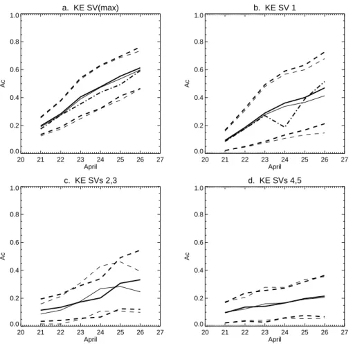
Next, we present the statistics of pattern correlations be-tween the 100 evolved error fields and SVs in the KE, EN and SF norms. Figures 8a, 9a and 9c depict these statistics for the largest pattern correlations taken over the five fastest growing SVs in the KE, EN and SF norms respectively and for both the viscous and inviscid cases. Again, for both the
viscous and inviscid cases, Figs. 8b, 9b and 9d show the cor-responding statistics for correlations between the error fields and SVs 1 in the KE, EN and SF norms respectively. Statis-tics of pattern correlations with SVs 2 and 3 (respectively 4 and 5) in the viscous case and for the KE norm are shown in Fig. 8c (respectively Fig. 8d). Also shown in Fig. 8a, for the viscous case, are the statistics for the largest pattern cor-relations taken over the five fastest growing FTNMs (thick dot-dashed line), and in Fig. 8b the statistics of pattern cor-relations with FTNM 1 (thick dot-dashed line).
We see from Figs. 8 and 9 that there is, in general, little difference in the results with and without viscosity, and the statistics of pattern correlations again increase monotonically with increasing time interval. We note that the mean pattern correlations with SVs in the KE and SF norms and with FT-NMs are, in general, very similar to each other and, after the first two days, slightly larger than those with SVs in the EN norm. All these mean pattern correlations are also larger than those with LVs shown in Fig. 7.
From the results presented in this section we can conclude that, after a few days, evolved, initially random, errors take up structures that are most similar to dominant SVs in the KE or SF norms or the dominant FTNMs. However, from Sect. 4, we know that the dominant SVs in SF and KE norms grow super-exponentially and that the amplification factors of the initially random error fields are more closely similar to those
a. KE SV(max) 20 21 22 23 24 25 26 27 April 0.0 0.2 0.4 0.6 0.8 1.0 Ac b. KE SV 1 20 21 22 23 24 25 26 27 April 0.0 0.2 0.4 0.6 0.8 1.0 Ac c. KE SVs 2,3 20 21 22 23 24 25 26 27 April 0.0 0.2 0.4 0.6 0.8 1.0 Ac d. KE SVs 4,5 20 21 22 23 24 25 26 27 April 0.0 0.2 0.4 0.6 0.8 1.0 Ac
Fig. 8. As in Fig. 7 but for KE SVs
re-placing LVs.
of the dominant FTNMs and LVs. The evidence for super-exponential growth of errors is discussed in the conclusions. In the following, we examine whether the results established here for April also apply in other situations of blocking.
5.2 December
The evolving structures of initially random errors during early December have also been analyzed. The qualitative results for our study covering the period 5 to 11 December are quite similar to the April results. For both December and April the dominant LVs are less similar to the dominant FTNMs than for November.
6 Statistics of error growth in November
In this section, we compare the properties of SVs, LVs and FTNMs during November with the structural development of initially random errors. We focus on the viscous case since, as found in the previous sections and confirmed for November (and December), the pattern correlations only de-pend weakly on the choice of dissipation. In particular, we analyze the statistics of the development of random errors during the period from 8 to 14 November when a blocking dipole structure became established over the Indian Ocean. We also examine whether the mean pattern correlations
be-tween random errors and dominant LVs, SVs and FTNMs increase further when the time interval is extended beyond the six-day period. We present results for the period from 1 to 15 November.
6.1 SVs, LVs and FTNMs in November
We begin with an examination of the structures of SVs, LVs and FTNMs. In calculating the LVs and MLVs for Novem-ber and DecemNovem-ber, we used the same procedure and stan-dard method as described in the April case. The randomly generated initial perturbations on 1 October 1989 are inte-grated (linearly) simultaneously with the time varying basic state that is obtained from observations. By doing so we have very good approximations of LVs for all the days in Novem-ber and DecemNovem-ber. Displayed in Figs. 10a and b are the fi-nal evolved EN SV 1 and KE SV 1 for the period from 8 to 14 November. Their structures are similar and also resemble that of the evolved SF SV 1 (not shown). The initial SVs 1 in the three different norms are again very different as ex-pected (not shown). The evolved SVs 1 are also similar to FTNM 1 for the same period shown in Fig. 10c and to LV 1 on 14 November shown in Fig. 10d. All the perturbations in Fig. 10 have large-scale dipole or multi-pole structures ex-tending downstream of the blocking region over the central Indian Ocean. The correlations of FTNM 1 with the evolved
a. EN SV(max) 20 21 22 23 24 25 26 27 April 0.0 0.2 0.4 0.6 0.8 1.0 Ac b. EN SV 1 20 21 22 23 24 25 26 27 April 0.0 0.2 0.4 0.6 0.8 1.0 Ac c. SF SV(max) 20 21 22 23 24 25 26 27 April 0.0 0.2 0.4 0.6 0.8 1.0 Ac d. SF SV 1 20 21 22 23 24 25 26 27 April 0.0 0.2 0.4 0.6 0.8 1.0 Ac
Fig. 9. Pattern correlations (Ac)
be-tween the dominant EN SVs, SF SVs and the 100 evolved random errors in both inviscid and viscous cases dur-ing the periods from 20 to 21, 22, . . ., 26 April 1989. Shown are (a) the mean (solid) and mean ± the standard devia-tion (dashed) of the largest correladevia-tions taken over the five fastest growing EN SVs (viscous - thick, inviscid - thin); (b) as in (a) but for the correlations between the 100 evolved random errors and EN SV 1; (c) as in (a) but for SF SVs; and
(d) as in (b) but for SF SV 1.
EN SV 1, KE SV 1 and SF SV 1 during the period from 8 to 14 November are 0.58, 0.59 and 0.72 respectively, similar to the April case. However, the structure of LV 1 on 14 Novem-ber is different from the April case in the sense that it has high correlations with FTNM 1 and the evolved SVs in all norms for the same period. These correlations are 0.66, 0.79, 0.85 and 0.49 for EN SV 1, KE SV 1, SF SV 1 and FTNM respectively.
We have also calculated SVs in the three norms for shorter periods ending on 14 November. We find, in particular, that the evolved KE SV 1 has a structure quite similar to that shown in Fig. 10a for optimization periods between one and six days. In contrast, for SF SV 1 and EN SV 1 the opti-mization periods need to be at least three and four days re-spectively to reproduce this evolved structure. It should be emphasized that, if the time interval is long enough, all the evolved SVs 1 will converge to LV 1 as discussed in Sect. 4.
6.2 Statistics of error growth during 8 to 14 November
For the period between 8 to 14 November, we again study the statistics of the growth of 100 error fields. The initial error fields on 8 November are random fields generated as described in Sect. 4. The period chosen covers the time in-terval of the development, maturation and decay of the Indian Ocean block.
Shown in Fig. 11 are the mean (solid) and the mean ± the standard deviations (dashed) of each pattern correlation of the evolved error field and final LVs, EN SVs, KE SVs and SF SVs on successive days. In Fig. 11a (thick lines), we dis-play these statistics for the largest correlations taken over the five fastest growing LVs for periods starting on 8 November and ending on subsequent successive days until 14 Novem-ber. The corresponding statistics for correlations between er-ror fields and LV 1 are also shown (thin lines), as are (in dot-dashed) the mean correlations taken over the five fastest growing FTNMs (thick dot-dashed) and mean correlation be-tween the 100 evolved errors and FTNM 1 (thin dot-dashed) for periods starting on 8 November. The same statistics for the evolved EN SV 1, KE SV 1 and SF SV 1 are shown in Figs. 11b–d respectively.
Figure 11 shows that the means (and the means ± the stan-dard deviations) of correlations taken over the five fastest growing LVs, SVs in each norm and FTNMs increase mono-tonically with time. The means in Fig. 11c and d (KE SVs and SF SVs) for the 6-day time interval are larger than those in Fig. 11b (EN SVs), which in turn are larger than those in Fig. 11a (LVs). The means taken over the five fastest growing FTNMs are again larger than those over the five fastest grow-ing LVs, although the differences are not as dramatic as for the April case shown in Fig. 7a. This appears to be related to the fact that in November the dominant LVs are more similar
Fig. 10. The streamfunctions of dominant dynamical vectors during the period between 8 to 14 November 1989 in the viscous case. Shown
are (a) the evolved EN SV 1 for 8 to 14 November, (b) the evolved KE SV 1 for 8 to 14 November, (c) FTNM 1 during 8 to 14 November and (d) LV 1 on 14 November.
to the dominant FTNMs than for April (Fig. 5b).
Again the means of correlations taken over the five fastest growing dynamical structures (SVs, LVs or FTNMs) are larger than those with the fastest growing dynamical struc-ture by itself. We also note that there is larger spread in the correlations with the fastest dynamical structure by itself than in correlations taken over the five fastest growing dynamical structures. On 14 November, after six days of integration, the mean correlation between the error fields and KE SV 1 is larger than those with the evolved EN SV 1 and SF SV 1
on this day and only slightly smaller than that with FTNM 1. As was the situation for April, on 14 November the mean correlation of the error fields with LV 1 is the smallest for the cases considered.
6.3 Statistics of error growth during 1 to 15 November
Next, we examine how the mean correlations between evolved error fields and the dominant LVs, SVs and FTNMs increase when the time interval is increased beyond six days.
a. LV(max), LV 1 8 9 10 11 12 13 14 15 Nov. 0.0 0.2 0.4 0.6 0.8 1.0 Ac b. EN SV(max), EN SV 1 8 9 10 11 12 13 14 15 Nov. 0.0 0.2 0.4 0.6 0.8 1.0 Ac c. KE SV(max), KE SV 1 8 9 10 11 12 13 14 15 Nov. 0.0 0.2 0.4 0.6 0.8 1.0 Ac d. SF SV(max), SF SV 1 8 9 10 11 12 13 14 15 Nov. 0.0 0.2 0.4 0.6 0.8 1.0 Ac
Fig. 11. The mean and mean ± the
standard deviation of the pattern cor-relations between each of the 100 er-ror fields and dynamical vectors (LVs, SVs and FTNMs) in November in the viscous case. Shown are (a) the mean (thick solid line) and mean ± the stan-dard deviation (thick dashed lines) of the largest pattern correlations taken over the five fastest growing LVs for pe-riods starting on 8 November and end-ing on subsequent successive days up until 14 November; the mean (thin solid line) and mean ± the standard deviation (thin dashed lines) of the pattern cor-relations between the 100 evolved er-ror fields and LV 1 for the same pe-riods; also shown are the mean of the largest pattern correlations taken over the five fastest growing FTNMs (thick dot-dashed), and the mean of the pattern correlations between the 100 evolved error fields and FTNM 1 for the same period (thin dot-dashed); (b) as in (a) but for EN SVs and without the statis-tics for FTNMs; (c) as in (b) but for KE SVs; and (d) as in (b) but for SF SVs.
Here, the 100 random error fields are initialized on 1 Novem-ber and are integrated up to 15 NovemNovem-ber. We have calcu-lated the dominant evolved LVs and SVs in the three norms optimized for the period from 1 to 15 November. Their structures on 15 November are all similar as might be ex-pected from the discussion in Sect. 4. The evolved structures on 15 November resemble those on 14 November (Fig. 10) but slightly displaced downstream.
In Fig. 12, we show the same statistics as in Fig. 11 but for the periods from 1 to 15 November. It is evident from Figs. 11 and 12 that the final mean pattern correlations between the error fields and these vectors are considerably larger for the 14-day period from 1 to 15 November than those for the 6-days period from 8 to 14 November. For the November period, the increase in the mean correlation of the 100 error fields with the any of the SVs, LVs or FTNMs over the first 6 days to 7 November is less than over the six days to 14 November as seen in Figs. 11 and 12. Thus, the more rapid convergence to the dynamical vectors appears to be re-lated to more rapid error growth during the second week of November when the Indian Ocean block grows and decays.
7 Discussion and conclusions
The structures and evolutions of finite-time SVs and LVs have been studied and compared with FTNMs growing on observed space-time basic states within a barotropic tangent linear model. We have employed time-dependent basic states that have been obtained by linear interpolation of observed daily 300-mb flow fields. As a consequence, the perturbation fields grow on basic states that closely follow the observa-tions.
The LVs, SVs and FTNMs have been computed for differ-ent periods of time in April, November and December 1989 in the Southern Hemisphere when blocks formed, amplified and decayed in the regions of Australia-New Zealand or in the central Pacific. The growth of ensembles of 100 random initial errors have been analysed during each of these peri-ods of blocking and we have studied the statistics of the error fields. The structures of the evolved error fields have also been compared with the structures LVs, FTNMs and SVs in three different norms.
The SF norm results in initial small-scale SV disturbances, the KE norm yields intermediate scale disturbances and the EN norm gives large-scale disturbances with large zonal flow components. After a few days, the structures of the dominant evolved SVs are much more similar with large-scale dipole or multi-pole structures in, and extending downstream from,
a. LV(max), LV 1 2 4 6 8 10 12 14 16 Nov. 0.0 0.2 0.4 0.6 0.8 1.0 Ac b. EN SV(max), EN SV 1 2 4 6 8 10 12 14 16 Nov. 0.0 0.2 0.4 0.6 0.8 1.0 Ac c. KE SV(max), KE SV 1 2 4 6 8 10 12 14 16 Nov. 0.0 0.2 0.4 0.6 0.8 1.0 Ac d. SF SV(max), SF SV 1 2 4 6 8 10 12 14 16 Nov. 0.0 0.2 0.4 0.6 0.8 1.0 Ac
Fig. 12. As in Fig. 11 but for the
peri-ods starting on 1 November and ending on subsequent successive days up until 15 November.
the blocking regions. After about three days, the evolved SVs also have structures which resemble some of the dominant FTNMs that are norm independent.
We have also calculated the dominant LVs, which have the largest long-time average growth rates, and the maxi-mum growth Lyapunov vectors 1 (MLVs 1), which are the Lyapunov vectors that at a given time have the largest local exponents or growth rates. For optimization times of six days or less, the evolved SVs and FTNMs are, in general, signifi-cantly different from the dominant LVs or MLVs on the same day. Nevertheless, the amplification factors of FTNMs 1 and LVs 1 are very similar, and also similar but slightly larger than the mean amplification factor of 100 initially random errors, while the amplification factors of SVs 1 in KE and SF norms are significantly higher than those of FTNMs 1 and LVs 1. The amplification factors of MLVs 1 are slightly higher than those of LVs 1 and FTNMs 1, but much lower than those of dominant SVs in KE and SF norms. However, in the SF norm, the amplification factors of EN SV 1 are lower than those of FTNM 1, LV 1 and the mean amplifica-tion factor of 100 initially random errors in either the inviscid or viscous case.
For longer optimization periods the evolved SVs increas-ingly turn towards the leading LV, which is norm indepen-dent. For periods of a month, the pattern correlations be-tween the leading SVs and leading LV are very close to 1
and the correlation between FTNM 1 and the leading LV is also very close to 1. The convergence of the leading SVs to the leading LV is expected on the basis of the Oseledec theorem.
The structural organization of initially random errors evolving in the barotropic tangent linear model has been compared with the dynamical vectors (SVs, LVs and FT-NMs). The mean and standard deviation of pattern corre-lations between each of 100 evolved error fields and the five fastest growing dynamical vectors (SVs, LVs and FTNMs) have been calculated. The mean of the largest pattern cor-relation taken over the five fastest growing SVs, in any of the three norms, or over the five fastest growing FTNMs, increases monotonically with increasing time interval to a value close to Ac=0.6 after six days. Thus, as far as
rep-resenting the structures of the evolved error fields is con-cerned, superpositions of five SVs or five FTNMs would be approximately equally skillful. In contrast, the correspond-ing mean taken over the five fastest growcorrespond-ing LVs only in-creases to a value of of less than Ac = 0.5 after six days.
In both April and December, these mean pattern correlations involving SVs or FTNMs are larger, by about a standard de-viation, than mean pattern correlations with LVs, for periods between a few days and six days.
The mean of pattern correlations with any of the indi-vidual five fastest growing dynamical vectors also generally
increases with time but not always monotonically. Dynami-cal vectors 1 (KE SV 1, SF SV 1, EN SV 1, FTNM1 or LV 1) generally, but not always, give the largest pattern correlations with the error fields. We have also examined the statistics of the convergence of error fields towards the dominant dynam-ical vectors for a longer 14-day period in November. At the end of this 14 day period, the mean pattern correlations be-tween perturbations and dynamical vectors are significantly larger than at the end of a six-day period. This is of course to be anticipated from the tendency of all disturbances to con-verge towards LV 1 with increasing time. We have also found that during periods of rapid error growth when blocks de-velop or decay, such as during the second week of Novem-ber, the error fields converge more quickly to the structures of the dynamical vectors than during more quiescent periods, such as during the first week of November.
We have found evolved error fields, starting from random perturbations, are slightly better described in terms of dom-inant FTNMs than in terms of domdom-inant LVs for the peri-ods considered. The growth rates of typical initially ran-dom errors are also comparable with those of the first 30 eigenvectors (Fig. 6) suggesting a representation in terms of the first 30 eigenvectors or 15 to 20 FTNMs would capture both the structure and growth of the error fields. At a given time, a representation in terms of dominant SVs would be as successful in capturing the structure of the evolved er-ror fields. However, since our erer-ror fields have been spec-ified to be initially random they do not, as expected, ex-hibit super-exponential growth. The issue of whether real meteorological analysis errors go through an initial phase of super-exponential growth is contentious, with, for ex-ample, Simmons et al. (1995) finding no clear evidence of super-exponential growth of initial errors in their study with the ECMWF numerical prediction model. On the other hand, a number of authors have presented evidence of super-exponential growth of large scale errors. This includes the studies of Schubert and Suarez (1989) with a simple gen-eral circulation model and the works of Trevisan (1993) with simple low order models. Nicolis et al. (1995) examined the mechanisms responsible for super-exponential growth in low order models. Frederiksen and Branstator (2001) have found that both large scale barotropic teleconnection pattern FT-NMs and travelling normal modes for zonally varying basic states can grow super-exponentially and sub-exponentially during parts of their life-cycles.
In a sequel to this work we plan to compare ensemble pre-diction schemes in which the control forecasts are perturbed by SVs, LVs and FTNMs.
Acknowledgements. It is a pleasure to thank S. Kepert for
assis-tance with this work. Edited by: A. Osborne Reviewed by: two referees
References
Anderson, J. L.: Selection of initial conditions for ensemble fore-casts in a simple perfect model framework, J. Atmos. Sci., 53, 22–36, 1996.
Arnoldi, W. E.: The principle of minimized iterations in the solution of the matrix eigenvalue problem, Quart. Appl. Math., 9, 17–29, 1951.
Benetin, G., Galgani, L., Giorgilli, A., and Strelcyn, J.-M.: Lya-punov characteristic exponents for smooth dynamical systems and forHamiltonian systems: a method for computing all of them. Part 1: Theory, Part 2: Numerical Application, Meccanica, 15, 9–30, 1980.
Branstator, G. and Haupt, S. E.: An Empirical Model of Barotropic Atmospheric Dynamics and Its Response to Tropical Forcing, J. Climate, 11, 2647–2667, 1998.
Buizza, R. and Molteni, F.: The role of finite-time barotropic in-stability during transition to blocking, J. Atmos. Sci., 53, 1675– 1697, 1996.
Buizza, R. and Palmer, T. N.: The singular-vector structure of the atmospheric global circulation, J. Atmos. Sci., 52, 1434–1456, 1995.
CMB: Climate Monitoring Bulletin, Southern Hemisphere, No. 39 April; No. 46, November; No.47, December 1989, National Cli-mate Centre, Bureau of Meteorology, Australia, 1989.
Corazza, M., Kalnay, E., Patil, D. J., Morss, R., Szunyogh, I., Hunt, B., York, J., and Cai, M.: Use of the breeding technique to estimate the structure of the analysis – “errors of the day”, Nonl. Proc. in Geoph., 10, 233–243, 2003.
de, Pondeca, M. S. F. A., Barcilon, A., and Zou, X.: An adjoint sensitivitystudy of the efficacy of modal and nonmodal pertur-bations in causing modelblock onset, J. Atmos. Sci., 55, 2095– 2118, 1998a.
de, Pondeca, M. S. F. A., Barcilon, A., and Zou, X.: The role of wavebreaking, linear instability, and PV transports in model block onset, J. Atmos. Sci., 55, 2852–2873, 1998b.
Farrell, B. F.: Optimal excitation of baroclinic waves, J. Atmos. Sci., 46, 1193–1206, 1989.
Farrell, B. F. and Ioannou, P. J.: Generalized stability theory. part II: nonautonomous operators, J. Atmos. Sci., 53, 2041–2053, 1996. Frederiksen, J. S.: A unified three-dimensional instability theory of the onset of blocking and cyclogenesis. II Teleconnection Pat-terns, J. Atmos. Sci., 40, 2593–2609, 1983.
Frederiksen, J. S.: Adjoint sensitivity and finite-time normal mode disturbances during blocking, J. Atmos. Sci., 54, 1144–1165, 1997.
Frederiksen, J. S.: Precursors to blocking anomalies: the tangent linear and inverse problems, J. Atmos. Sci., 55, 2419–2436, 1998.
Frederiksen, J. S.: Subgrid-scale parameterizations of eddy-topographic force, eddy viscosity and stochastic backscatter for flow over topography, J. Atmos. Sci., 56, 1481–1494, 1999. Frederiksen, J. S.: Singular vectors, finite-time normal modes, and
error growth during blocking, J. Atmos. Sci., 57, 312–333, 2000. Frederiksen, J. S. and Bell, R. C.: North Atlantic blocking during January 1979: Linear theory, Quart. J. Roy. Meteor. Soc., 116, 1289–1313, 1990.
Frederiksen, J. S. and Branstator, G.: Seasonal and intra seasonal variability of large-scale barotropic modes, J. Atmos. Sci., 58, 50–69, 2001.
Frederiksen, J. S. and Davies, A. G.: Eddy viscosity and stochas-tic backscatter parameterizations on the sphere for atmospheric