Validation of stratospheric water vapour measurements from the airborne microwave radiometer AMSOS

(1)

HAL Id: hal-00303275

https://hal.archives-ouvertes.fr/hal-00303275

Submitted on 30 Jan 2008

HAL is a multi-disciplinary open access

archive for the deposit and dissemination of sci-entific research documents, whether they are pub-lished or not. The documents may come from teaching and research institutions in France or abroad, or from public or private research centers.

L’archive ouverte pluridisciplinaire HAL, est destinée au dépôt et à la diffusion de documents scientifiques de niveau recherche, publiés ou non, émanant des établissements d’enseignement et de recherche français ou étrangers, des laboratoires publics ou privés.

Validation of stratospheric water vapour measurements

from the airborne microwave radiometer AMSOS

S. C. Müller, N. Kämpfer, D. G. Feist, A. Haefele, M. Milz, N. Sitnikov, C.

Schiller, C. Kiemle, Jakub Urban

To cite this version:

S. C. Müller, N. Kämpfer, D. G. Feist, A. Haefele, M. Milz, et al.. Validation of stratospheric water vapour measurements from the airborne microwave radiometer AMSOS. Atmospheric Chemistry and Physics Discussions, European Geosciences Union, 2008, 8 (1), pp.1635-1671. �hal-00303275�

(2)

ACPD

8, 1635–1671, 2008 Validation of water vapour measurements from AMOS S. C. M ¨uller et al. Title Page Abstract Introduction Conclusions References Tables Figures ◭ ◮ ◭ ◮ Back Close

Full Screen / Esc

Printer-friendly Version Interactive Discussion

Atmos. Chem. Phys. Discuss., 8, 1635–1671, 2008 www.atmos-chem-phys-discuss.net/8/1635/2008/ © Author(s) 2008. This work is licensed

under a Creative Commons License.

Atmospheric Chemistry and Physics Discussions

Validation of stratospheric water vapour

measurements from the airborne

microwave radiometer AMSOS

S. C. M ¨uller1, N. K ¨ampfer1, D. G. Feist2, A. Haefele1, M. Milz3,*, N. Sitnikov4, C. Schiller5, C. Kiemle6, and J. Urban7

1

University of Bern, Bern, Switzerland 2

Max-Planck-Institute for Biogeochemistry, Jena, Germany 3

Institut f ¨ur Meteorologie und Klimaforschung, Karlsruhe, Germany 4

Central Aerological Observatory, Moscow Region, Russia 5

Forschungszentrum J ¨ulich GmbH, J ¨ulich, Germany 6

DLR, Institut fuer Physik der Atmosphaere, Oberpfaffenhofen, Germany 7

Chalmers University of Technology, G ¨oteborg, Sweden *

now at: Lule ˚a Technical University, Kiruna, Sweden

Received: 13 November 2007 – Accepted: 20 December 2007 – Published: 30 January 2008 Correspondence to: S. C. M ¨uller (stefan.mueller@mw.iap.unibe.ch)

(3)

ACPD

Full Screen / Esc

Abstract

We present the validation of a water vapour dataset obtained by the Airborne Mi-crowave Stratospheric Observing System AMSOS, a passive miMi-crowave radiometer operating at 183 GHz. Vertical profiles are retrieved from spectra by an optimal es-timation method. The useful vertical range lies in the upper troposphere up to the

5

mesosphere with an altitude resolution of 8 to 16 km and a horizontal resolution of about 57 km. Flight campaigns were performed once a year from 1998 to 2006 mea-suring the latitudinal distribution of water vapour from the tropics to the polar regions. The obtained profiles show clearly the main features of stratospheric water vapour in all latitudinal regions. Data are validated against a set of instruments comprising

satel-10

lite, ground-based, airborne remote sensing and in-situ instruments. It appears that AMSOS profiles have a dry bias of 3–20%, when compared to satellite experiments. A good agreement with a difference of 3.3% was found between AMSOS and in-situ hygrosondes FISH and FLASH and an excellent matching of the lidar measurements from the DIAL instrument in the short overlap region in the upper troposphere.

15

1 Introduction

Water vapour is important for our environment and climate. It is a key element in the radiative budget of the earth’s atmosphere and contributes the largest to the green-house effect due to strong absorption in the troposphere. In the stratosphere water vapour is a source for the formation of polar stratospheric clouds and the OH radical

20

molecule and thus it is involved in the process of ozone depletion. In the mesosphere it becomes destroyed by photolysis. As a long-lived trace gas it provides the possibility to study atmospheric motion. The importance of knowledge about this key parameter is evident.

A very common technique to measure water vapour is by passive remote

sens-25

ing in the infrared or microwave regions by satellite, aircraft or ground-based instru-1636

(4)

ACPD

Full Screen / Esc

ments. Other techniques use in-situ sensors such as FISH (Z ¨oger et al., 1999) and FLASH (Sitnikov et al., 2007) from balloon or aircraft, or active remote sens-ing with differential absorption lidar (Ehret et al., 1999). Satellite observations have been made by UARS/HALOE (Russell III et al.,1993), ERBS/SAGE-II (Chiou et al.,

1997), SPOT4/POAM-III (Lucke et al.,1999), Aura/MLS (Schoeberl et al.,2006),

En-5

visat/MIPAS (Fischer et al., 2007) and Odin/SMR (Urban et al., 2007) over the last two decades and deliver an excellent three dimensional global coverage of the water vapour distribution. From aircraft a two dimensional snapshot of the water vapour dis-tribution along the flighttrack is obtained on a short timescale. Because stratospheric water vapour has a latitudinal dependence the main distribution patterns can be

mea-10

sured by a flight from northern latitudes to the tropics. Ground-based (Deuber et al.,

2004) (Nedoluha et al., 1995) or balloon soundings determine the one-dimensional

distribution on a continuous time basis and thus are very interesting for local trend analyses.

With the Airborne Microwave Stratospheric Observing System (AMSOS), carried by

15

a Learjet-35A of the Swiss Airforce, we measured the latitudinal distribution of water vapour from the tropics to the north pole during one week per year from 1998 to 2006. A former version of the instrument had been flown from 1994 to 1996 (Peter,1998). The instrument was flown in spring or autumn during active stratospheric periods due to the change between polar night-time and day-time. Measurements inside the polar vortex

20

as well as in the tropics including one overflight of the equator were accomplished. The dataset overlaps several satellite experiments in time. In a previous work (Feist et al.,

2007) this dataset has been compared to the ECMWF model.

In this paper we first present the AMSOS retrieval characteristic of the version 2.0 data and the 9-year AMSOS water vapour climatology of the northern hemisphere.

25

Secondly the validation of the data which has been performed against already vali-dated datasets from satellite experiments (Harries et al., 1996), (Rind et al., 1993), (Nedoluha et al.,2002), (Milz et al.,2005), (Raspollini et al.,2006), the ground-based station MIAWARA (Deuber et al.,2005) for the whole profile range, as well as with

(5)

ACPD

Full Screen / Esc

situ and lidar measurements in the UTLS region. The advantage of this dataset is its coverage of all latitudes from −10◦ to 90◦ North for the UTLS region up to the meso-sphere for early spring and autumn periods with a good horizontal resolution of 57 km. The data are useful for studies of atmospheric processes and validation. The profiles are available for download athttp://www.iapmw.unibe.ch/research/projects/AMSOS.

5

2 AMSOS water vapour measurement and retrieval

2.1 Measurement method

AMSOS measures the rotational emission line of water vapour at 183.3±0.5 GHz (Vasic

et al.,2005) by up-looking passive microwave radiometry (Janssen,1993). Performing observations at this frequency is dependent on atmospheric opacity. Figure1shows a

10

set of spectra measured at different flight altitudes during the ascent of the aircraft over the tropics. Under humid conditions as encountered in the tropics the line is saturated up to an altitude of more than 9 km. On the other hand in polar regions it is possible to make good quality measurements at flight levels down to approximately 4 km. Under very dry conditions in the winter months it is also possible to retrieve stratospheric

15

water vapour from the alpine research station Jungfraujoch in Switzerland at 3.5 km altitude for about seven percent of the time (Siegenthaler et al.,2001).

The AMSOS instrument was flown with a broadband accousto-optical spectrometer (AOS) of 1 GHz bandwidth during all missions, a broadband digital FFT spectrometer with the same bandwidth and a narrowband digital FFT spectrometer with bandwidth of

20

25 MHz only in 2005 and 2006. In this work only profiles from the AOS are presented.

2.2 AMSOS profile retrieval setup, characteristic and error analysis

For the retrieval of water vapour profiles from the measured spectra we need knowl-edge of the relationship between the atmospheric state x and the measured signal y.

(6)

ACPD

Full Screen / Esc

This is described by the forward model function F (Eq. 1). To find a solution for this inverse problem, we use the optimal estimation method (OEM) according to Rodgers (Rodgers,2000). The forward model is splitten up in a radiative transfer part

F_r calculated by theAtmospheric Radiative Transfer Simulator (ARTS) (Buehler et al.,

2005) and a sensor modelling part F_s which is done by the software package Qpack

5

(Eriksson et al.,2005). The implementation of the retrieval algorithm is also done by Qpack. Forward model parameters b like the instrument influencing the measurement namely antenna beam pattern, sideband filtering, observation angle, attenuation due to the aircraft window, standing waves, as well as atmospheric parameters like pres-sure and temperature profiles, other species, spectral parameters and line shape. ǫ is

10

the measurement noise.

y_{=F (x, b)+ǫ=F}_s[Fr(x, b)] +ǫ (1)

Inverse problems are often ill-posed and lead to a best estimate ˆx of the real state by minimising the so called cost-function

(y−(x, b))TS−1y (y−F (x, b))+(x−xa)TS−1x (x−xa) (2)

15

with the help of apriori information of the retrieval quantity xa, the measured spectrum

yand their covariance matrices Sxand Sy. The best estimate ˆx is found by an iterative

process with the Marquardt-Levenberg approach.

x_i₊₁₌ x_i_+(S−1_a _+KT_iS−1y Ki+γD)−1

{KT_iS−1y [y − [F (xi)]−S−1a [xi−xa]} (3)

20

where Ki =

∂F(xi,b)

∂xi , γ a trade-off parameter and D a diagonal scaling matrix.

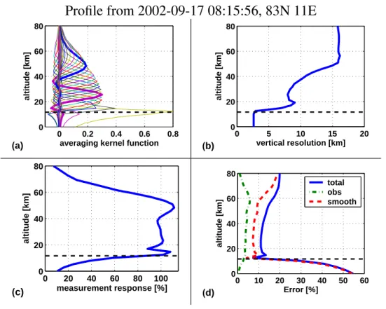
The character of a retrieval is derived from the averaging kernel matrix A=A(K, Sx,

Sy). An example is given in Fig.2a). A also provides information about the

measure-ment response that is a measure of how much the retrieved profile depends on the measurement and how much on the apriori profile by taking the integral over A. The

25

(7)

ACPD

Full Screen / Esc

full width at half maximum of each averaging kernel function represented by a row in the matrix A provides the vertical resolution. A typical averaging kernel matrix A, the meaurement response and the vertical resolution of a retrieval from AMSOS is shown in Fig.2a–c. Between approximately the flight altitude and 60 km the measurement re-sponse is more than 80%. The vertical resolution ranges between 8-16 km increasing

5

with altitude. The trace of A is an indicator for the number of independent points and is between 4–6 for AMSOS. Qpack takes into consideration the model uncertainties and the measurement error and the error of the apriori profile, called the smoothing error. The total error is in the order of 10–15% for the altitudes with apriori contribution less than twenty percent (Fig. 2d). The smoothing error part is almost the double of the

10

observation error.

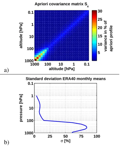
2.3 Water vapour apriori information, covariance matrix and model parameters An important issue for processing our AMSOS dataset was the selection of an ap-propiate apriori water vapour profile to constrain the retrieval algorithm to a reasonable solution. We made the choice to use a global mean of monthly means of the ERA40

15

climatology from ECMWF from ground up to 45 km. To build the mean profile we intro-duced a latitudinal weight to avoid an overweight of polar profiles since the number of ECMWF grid points per latitude is constant. Out of the statistic of these 425 000 pro-files we set up the covariance matrix S_xas shown in Fig. 3a. The standard deviation (Fig.3b) in the stratosphere is lower than 10% and in the troposphere it raises up to

20

80%. This change is directly visible in the diagonal elements of the coavriance matrix

Sx. For altitudes above the ERA40 grid we used the US-Standard Atmosphere (U.S.

Committee on Extension to the Standard Atmosphere,1976) as apriori information. For the temperature and pressure profiles we used data from ECMWF continued by CIRA86 (Rees et al., 1990) for the altitude levels above the top of the ECMWF

25

atmosphere. Spectral parameters are taken from the HITRAN96 (Rothman et al.,1998) molecular spectroscopy database.

Additionally a baseline which originates from a standing wave between the mixer 1640

(8)

ACPD

Full Screen / Esc

and the aircraft window, resulting in a sinusoidal modulation of the spectrum with a frequency of 75 MHz, and a constant offset of the spectrum is retrieved.

2.4 Spectra pre-integration

To reduce thermal noise to approximately 1% before retrieving a profile we had to pre-integrate several spectra. It is important to pre-integrate spectra that were measured under

5

similiar conditions. The most critical parameters that could change quickly during flight are the flight altitude and the instrument’s elevation angle. The elevation angle depends on the aircraft’s roll angle as well the position of the instrument’s elevation angle. Only spectra with a maximum roll angle difference of ±0.1◦, a mirror elevation of ±0.1◦ and a flight altitude within ±100 m were integrated. To avoid integration of spectra over

10

a too large distance, the spectra were only considered if they were measured within 10 min. This finally determines the horizontal resolution along the track of 57 km±30 km of the AMSOS dataset. The remaining noise that overlay the spectrum determines the diagonal elements of the covariance matrix of the measurement error of Sy.

2.5 AMSOS campaigns and dataset

15

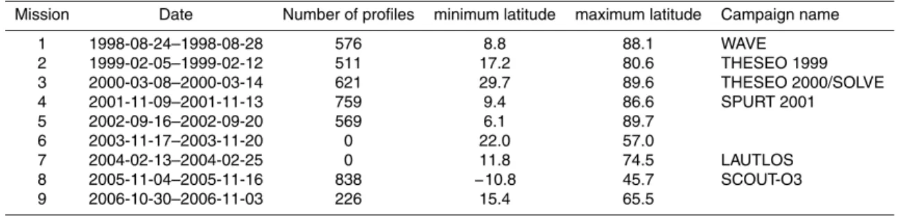
The here presented AMSOS dataset contains 4100 profiles presented in Fig. 4 from flight campaigns or missions between 1998 and 2006 as overviewed in Table 1 and Fig.6. The instrument participated often as a part of international campaigns during this period. In most cases the flight route was planned to cover as many latitudes as possible between the equator and the north pole. The AMSOS flight track is indicated in

20

blue for each mission in Fig.6where every plot is dedicated to one campaign. During participation in the SCOUT-O3 Darwin campaign in 2005 our track was in east-west direction including an overpass of the equator (see Fig.6f).

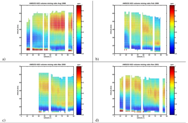
Every flight mission presented in Fig. 4 by altitude latitude plots show a very dry stratosphere with no more than 4 ppm volume mixing ratio over the tropics up to 40 km.

25

In the mid-latitudes and polar region values of 5 ppm are reached down to 20 km. In 1641

(9)

ACPD

Full Screen / Esc

the upper stratosphere the increase of water vapour generated by methane oxidation resulted in measurements at 50 km of up to 7 ppm. Above decreasing water vapour induced by photolysis was observed. In the November and February/March missions numbered 2, 3, 4 and 9 (see Fig.4b, c, d and g) the water vapour maximum subsided to a level of 35 km above the Arctic. The upper troposphere as a wet layer above the

5

aircraft is visible in all missions that is elevated in the tropics in contrast to the Arctic. For additional discussions see (Feist et al.,2007).

3 AMSOS validation

3.1 Comparison technique

When comparing data from two remote sensing instruments their vertical resolution

10

has to be considered. Let us assume the instrument to compare with has a higher resolution. Applying the averaging kernels A according to Eq. 4 reduces its vertical resolution to the resolution of the lower resolved profile and smoothes out fine struc-tures.

ˆ

x_=x_a_+A(x−x_a) (4)

15

where x is the high resolution and ˆx its equivalent reduced resolution profile from the comparative instrument. This is a technique already used for comparisons between low and high resolution remote sounders by (Connor et al., 1995) and (Tsou et al.,

1995).

In our case it was necessary to do a small modification due to the character of the

20

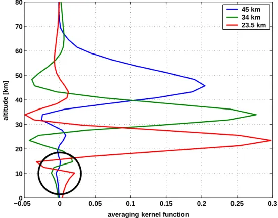
water vapour profile and our possibility to measure in the upper troposphere. Below the hygropause water vapour increases exponentially. The term (x−xa) in (4) can become very large for different hygropause levels in x and xa. An averaging kernel function corresponding to a certain altitude level is minimal but not necessarily zero below the hygropause level as shown in Fig. 5 and consequently contribute significantly to the

25

(10)

ACPD

Full Screen / Esc

values of the smoothed profile in the upper stratosphere. Since our apriori profile is global and the altitude level of the hygropause changes with latitude this effect is encountered quite often. To get rid of this, we must apply the averaging kernels from hygropause level upwards and lower down we take the direct difference of the profile.

This approach is used to compare the AMSOS measurements with the higher

re-5

solved limb sounding profiles from satellite observations and the microwave ground-station MIAWARA. For the comparisons to the in-situ instruments FISH and FLASH we interpolated on the same grid. Concerning the differential absorption lidar we plotted the independent profiles in the interesting overlap region in the UTLS.

3.2 Comparisons with other instruments

10

For an ideal validation study instruments measuring water vapour at almost the same place at the same time are needed. By flying directly over a ground-based station the constraint of place and time can be satisfied easily, as well as for the case of flying in parallel with another aircraft. In case of crossing the footprint of a satellite-based instrument a certain space and time frame has to be selected as the satellite and

15

aircraft paths are not crossing at the same time or only nearby.

During each flight mission we can find at least one collocation of an AMSOS profile and a satellite experiment within a radius of 500 km and a time difference of 10 h. Comparative satellite experiments were the SPOT4/POAM-III (data down-loaded from ftp://poamb.nrl.navy.mil/pub/poam3/), ERBS/SAGE-II (data downloaded

20

from http://badc.nerc.ac.uk/data/sage2/), Uars/HALOE (data downloaded from http:

//haloedata.larc.nasa.gov/), Aura/MLS (data downloaded from http://daac.gsfc.nasa.

gov/Aura/MLS/), Envisat/MIPAS and Odin/SMR. In case of the MIPAS instrument the comparison was available using two different datasets from the European Space Agency (ESA) and the Institut fr Meteorologie und Klimaforschung (IMK), Karlsruhe,

25

Germany. This set of satellite experiments observing at different times makes the AMSOS instrument also useful for cross-validation studies by the technique given in (Hocke et al.,2006).

(11)

ACPD

Full Screen / Esc

During the transfer flight of the SCOUT-O3 Darwin campaign, the Learjet has flown in parallel with the two aircrafts DLR Falcon 20 and the russian Geophysica M55. On-board the Falcon a Differential Absorption Lidar (DIAL) (Ehret et al.,1999) system was operated to measure the water vapour above the aircraft up to an altitude of about 17 km. This gave an overlap region with the AMSOS profile in the upper troposphere

5

letting us combine the water vapour profiles from two different systems. Finally, we compared our data with the instruments FISH and FLASH, which both use the

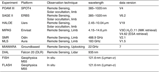
Lyman-αline in the UV and perform in-situ measurements from the Geophysica aircraft. An overview of all the insruments is given in Table 2. The whole set of instru-ments used for comparison include different remote sensing and in-situ techniques,

10

passive and active methods, occultation, limb and up-looking, ground-based, airborne and satellite borne, and cover the electromagnetic spectrum from the ultraviolet to the microwave region.

3.3 Validation with observations from satellites

For the purpose of validation at all altitudes we compared the dataset to the six

satel-15

lite experiments mentioned in Sect.3.2. Figure 6 shows all the collocation pairs with satellite sensors for all AMSOS missions. For each mission there is at least one collo-cation pair that matches the criteria of being within a radius of 500 km and 10 h of time. The criteria was chosen as large that we could find collocation pairs and the profiles do not originate from totally different air masses. We found about 10 matching profiles

20

in the first four AMSOS missions with SPOT4/POAM-III and 2 with ERBS/SAGE-II. These two satellite experiments are solar occultation instruments and thus only per-formed measurements during sunrise and sunset while the AMSOS instrument was flying mostly during daytime. With the Uars/HALOE instrument which also accom-plished solar occultation measurements only two collocations were found in mission

25

5. In the same mission there are more than fourty coinciding measurements with En-visat/MIPAS which is a full-time measuring instrument. In the last two AMSOS missions several track crossings with the Aura satellite resulted in more than 75 collocation pairs

(12)

ACPD

Full Screen / Esc

with the MLS instrument.

The comparison is done over the altitude region where the measurement response of the AMSOS profile is larger than 50% or until no more information of the satellite is available. Profile differences were plotted in relative units according to

∆VMR[%] = VMRAMSOS− VMRInstrument

VMR_Instrument . (5)

5

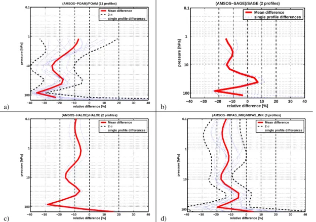
In Fig.7 the thick red line is the mean relative difference of all the single difference profiles in dotted blue. The offset is negative when AMSOS measures drier values and positive when AMSOS has a wet bias.

The comparison to the POAM-III instrument (Fig.7a) shows a relative difference of −35% at 90 hPa and then decreases below −10% at 1 hPa with respect to AMSOS.

10

SAGE-II (Fig. 7b) shows a bias of −22% at 90 hPa which turns to positive values in the lower stratosphere before the mean difference is stabilized at −12% between 10 and 1 hPa. Also HALOE (Fig.7c) shows a −29% offset at the 90 hPa level and a quasi constant offset of 10% up to 0.1 hPa. Both HALOE and SAGE-II with only two collocations did not issue additional statistical information but nevertheless they show

15

the same typical features in the mean difference profile as the others.

In case of the MIPAS instrument we compared to two different independent retrievals. On the one hand the IMK (Fig.7d) retrieval and on the other hand (Fig.7e) the ESA operational retrieval. Collocations with IMK profiles do not cover latitudes northerly than 66◦N. Both profile sets show a similar behaviour. Again the 90 hPa level is offsetted by

20

−20% (IMK) to −25% (ESA). At 30 hPa it changes to −5% (IMK) and no offset (ESA). Between 10 and 0.1 hPa the offset is −15% in the mean for both. In case of the ESA retrieval it is slightly decreasing in this altitude range.

The two profiles of the Odin/SMR instrument compare well with the AMSOS instru-ment. The error amounts between −15% and +5% in the altitude range of 60 to

25

0.1 hPa. It is slightly positive between 1 and 10 hPa. But also here the number of collocations is too low to make a statistical conclusion.

(13)

ACPD

Full Screen / Esc

The Aura/MLS instrument using the same observation frequency as AMSOS also shows a clearly offset of −20% at the 90 hPa level. Throughout the stratosphere it is similar to the HALOE comparison at −10% and increasing to −20% in the lower mesosphere between 0.1 and 1 hPa. This maybe due to increasing apriori contribution in the AMSOS profiles at these altitudes.

5

For the lower stratosphere and the hygropause region in Fig. 7a–g, apart from the offset the mean difference profile shows an oscillation in the order of ±15% between 100 and 10 hPa appearing in all comparisons with collocations north of 45◦. In the upper troposphere the mean difference is positive which is caused by a vertical offset of the hygropause level and a strong gradient of water vapour mixing ratio below the

10

hygropause. According to the ground-based MIAWARA profile there is a slightly dry bias in the lower stratosphere and a slightly wet bias in the upper stratosphere of ±10% (see Fig.7).

3.4 Validation with the ground-station MIAWARA

There was one coinciding measurement with the ground-based microwave

radiome-15

ter MIAWARA (Deuber et al., 2005) in Bern, Switzerland on 16th November 2005. Because the MIAWARA instruments vertical resolution is lower than the one from AM-SOS we applied the MIAWARA averaging kernels to the AMAM-SOS profile according to the technique in Sect.3.1. The left hand side of Fig.8shows both the AMSOS and the MIAWARA profile. Taking the relative difference resulted in an agreement of slightly

de-20

creasing from −10 to 0% in altitudes between 30 and 0.3 hPa where the measurement response of both instruments is larger than 0.5.

3.5 Latitude dependence

As seen in Sect.3.3all the mean difference profiles of the comparisons to the satellites show a negative peak at the 90 hPa level. It seems to be a character of the AMSOS

25

profile to be very dry around the hygropause. When analyzing the locations of the collo-1646

(14)

ACPD

Full Screen / Esc

cations most of them originate in the mid-latitudinal to polar region. With the Aura/MLS and Envisat/MIPAS instruments which collocations with AMSOS cover additionally the subtropical region we separated the profile comparisons in two geographical regions, the first from 90◦N to 45◦N and the second from 45◦N to 0◦N. As shown in Fig. 9the mean difference profile is dependant on latitude. The characteristical peak is visible

5

for both only in the profiles north of 45◦N. In case of the MIPAS instrument the two mean difference profiles differ only in the UTLS region up to 10 hPa while the two MLS regional mean difference profiles are slightly offsetted by less than 10% over the whole altitude range.

The origin of this peak at 90 hPa can be explained by an elevated hygropause in

10

the AMSOS profiles that would exactly produce this effect when taking the difference. The reason why this appears only in the polar profiles is hidden in the apriori profile of AMSOS and its covariance matrix. In polar regions the hygropause is located at a lower altitude level than in tropical or mid-latitudinal regions. The location of the hygropause in the apriori profile represents more a mid-latitudinal or sub-tropical case.

15

The constraint of the apriori covariance matrix Sxin the upper troposphere retained the

hygropause of the AMSOS profiles on a certain altitude level which is higher than other instruments have measured and lead to this peak at 90 hPa. The effect disappears between tropical and mid-latitudinal regions.

3.6 Wavelength dependence

20

The AMSOS comparisons includes passive remote sensing instruments observing at different wavelengths over a wide part of the electromagnetic spectrum. Illustrated in Fig.10is the mean bias over the vertical range from 120 to 0.1 hPa as a function of the wavelength of the sensor. By color coding we grouped optical, infrared and microwave instruments together. The mean bias to AMSOS seems to decrease with increasing

25

sensor wavelength. Calculating the group mean we get for the optical −14.4%, the infrared −11.7% and for the microwave sensors −7.5%. A possible explanation could be found in the uncertainties in the spectral line catalogues for the line broadening and

(15)

ACPD

Full Screen / Esc

intensity parameters. Table3shows a composition of line broadening parameters of the 183.31 GHz water vapour line out of the HITRAN and JPL catalogue and a laboratory measurement by (Tretyakov et al.,2003). Differences in line amplitude, air broadening width and its temperature exponent are already visible over the different catalogues for the same molecular transition. It might differ also over the different spectral regions

5

and thus lead to offsetted profiles. This hypothesis will further be treated in (Milz et al., in preparation).

3.7 Validation of AMSOS upper tropospheric humidity with lidar profiles

In each viewgraph of Fig.11we plotted the corresponding profiles from the two differ-ent measuremdiffer-ent techniques lidar and microwave covering differdiffer-ent altitude regions.

10

Profiles are averaged over 1 degree in longitude. The lidar profile from the DIAL in-strument reaches the upper troposphere where the AMSOS inin-strument starts to be sensitive to water vapour. 8 cases from the mid-latitudes to the tropics are presented here. The lidar profiles match into the 2σ error of the AMSOS profile. The different gradients in the profiles is clearly visible in the first case of Fig.11(41 N,17 E) originate

15

in the limited vertical resolution of the microwave instrument. The fine structure nicely seen in the lidar profile in case 7 (14 N, 100 E) can not be seen by AMSOS either. The last three profiles of Fig.11were in the presence of cirrus clouds extending up to 17 km at 16 N, 90 E.

3.8 Validation with in-situ hygrometers FISH and FLASH

20

On the transfer flight of the SCOUT-O3 Darwin campaign we had the possibility to fly in parallel with the Lyman-α hygrometers FISH and FLASH that were carried by the air-craft Geophysica-M55. The measurements for this comparison were averaged to one degree in longitude along the flight track. As shown in Fig.12b) aircraft Geophysica-M55 was flying above hygropause level and, except for the path between 110◦and 130◦

25

longitude, the measurements fit within the 2σ errorbars of the AMSOS instrument (see 1648

(16)

ACPD

Full Screen / Esc

Fig.12a). Looking more into detail of the path between 110◦ and 130◦ we can identify in the ECMWF profile in Fig.12c) a small very dry layer near the hygropause where Geophysica was located. Due to the limited altitude resolution AMSOS did not detect this feature of the water vapour profile. Excluding these last measurements AMSOS has a dry bias of 3.3%±15% with respect to FISH and FLASH.

5

4 Summary and conclusions

The AMSOS water vapour dataset consists of more than 4000 profiles from the UTLS region up to the mesosphere covering all latitudes from tropical to polar regions with good horizontal resolution of 57 km. The airborne instrument was running for approx-imately one week a year between 1998 and 2006. The main features of the vertical

10

water vapour distribution are clearly seen by the radiometer despite the limited altitude resolution of 8–16 km. The upper tropospheric part with the strong gradient in water vapour is visible as well as the water vapour maximum, which is the main feature in the stratosphere, as a footprint of methane oxidation and transport by the Brewer-Dobson circulation. The water vapour minimum, also known as the hygropause, is apparent

15

over the tropics at a higher altitude level than over the Arctic. In the late winter mis-sions of 1999 and 2000 and the late autumn mismis-sions of 2001 and 2006 lower water vapour values were measured in the Arctic upper stratosphere compared to the late summer missions of 1998 and 2002. Due to the subsidence of air over the pole by Brewer-Dobson circulation and on the other hand also an effect of the polar vortex that

20

builds a barrier for the transport of mid-latitudinal air masses towards the pole.

Validation of the whole dataset in the different years of measurements and over the whole geographical region was successfully done with a large set of different instru-ment types using different data collection methods and different data processing algo-rithms. Comparisons with satellite borne passive remote sensing instruments show a

25

dry bias of the AMSOS instrument in the order of 3–20%. This variability of the bias of the passive remote sensing instruments seems to be dependent on the wavelength

(17)

ACPD

Full Screen / Esc

of the observation frequency. Forming sensor groups based on the typical spectral re-gions optical, infrared and microwave seems that the offset is decreasing with sensor wavelength. A hypothesis is the remaining uncertainty in the spectral parameters used in the forward model in the inversion process but this needs further investigations. A second bias dependency appears with latitude. A typical mean difference profile in the

5

Arctic has a sharp peak at the 90 hPa level while this does not appear in the tropi-cal profiles as seen in the comparisons with MLS and MIPAS. The characteristic peak is also visible in comparisons with HALOE, SAGE-II and POAM-III data which have collocations only in the Arctic. The global apriori of the AMSOS dataset and its co-variance matrix constrain the tropospheric part too strongly which leads to an elevated

10

hygropause level for retrieved polar AMSOS profiles. With the in-situ instruments FISH and FLASH during SCOUT-O3 campaign in 2005 the agreement with a discrepancy in the order of 3.3% is excellent for non special conditions as was the case for flightlegs 1–4. If the sondes are flying inside small fine water vapour structures such as during flightlegs 5 and 6 then AMSOS is not able to resolve this fine structure. An excellent

15

matching of lidar profiles from DIAL and the AMSOS microwave profiles in the upper troposphere was also found during SCOUT-O3. Thus a combination of a lidar and a microwave radiometer allowed to measure water vapour from the troposphere up to the mesosphere during the SCOUT-O3 campaign.

Mesospheric water vapour profiles up to an altitude of 75 km retrieved from a different

20

spectrometer will be added to the dataset later.

Acknowledgement. S. C. M ¨uller’s work was supported by the Swiss National Science

Founda-tion under grant 200020-115882. We would like to thank the Swiss Air Force for providing the aircraft and especially the aircraft pilots for their excellent support during the flight campaigns. We thank also the ECMWF, HALOE, ESA, AURA, POAM and SAGE teams for providing their

25

data.

(18)

ACPD

Full Screen / Esc

References

Buehler, S. A., Eriksson, P., Kuhn, T., von Engeln, A., and Verdes, C.: ARTS, the Atmo-spheric Radiative Transfer Simulator, J. Quant. Spectrosc. Radiat. Transfer, 91, 65–93, doi:10.1016/j.jqsrt.2004.05.051, 2005. 1639

Chiou, E., McCormick, M., and Chu, W.: Global water vapor distributions in the stratosphere

5

and upper troposphere derived from 5.5 years of SAGE II observations (1986–1991), J. Geophys. Rese, 102, 105–118, doi:10.1029/97JD01371, 1997. 1637

Connor, B. J., Parrish, A., Tsou, J.-J., and McCormick, M. P.: Error analysis for the ground-based microwave ozone measurements during STOIC, 100, 9283–9291, doi:10.1029/94JD00413, 1995. 1642

10

Deuber, B., K ¨ampfer, N., and Feist, D. G.: A new 22-GHz Radiometer for Middle Atmospheric Water Vapour Profile Measurements, IEEE Transactions on Geoscience and Remote Sens-ing, 42, 974–984, doi:10.1109/TGRS.2004.825581, 2004. 1637

Deuber, B., Haefele, A., Feist, D. G., Martin, L., Kampfer, N., Nedoluha, G. E., Yushkov, V., Khaykin, S., Kivi, R., and Vomel, H.: Middle Atmospheric Water Vapour Radiometer –

MI-15

AWARA: Validation and first results of the LAUTLOS/WAVVAP campaign, J. Geophys. Res., 110, D13306, doi:10.1029/2004JD005543, 2005. 1637,1646

Ehret, G., Hoinka, K. P., Stein, J., Fix, A., Kiemle, C., and Poberaj, G.: Low strato-spheric water vapor measured by an airborne DIAL, J. Geophys. Res., 104, 351–359, doi:10.1029/1999JD900959, 1999. 1637,1644

20

Eriksson, P., Jimenez, C., and Buehler, S. A.: Qpack, a general tool for instru-ment simulation and retrieval work, J. Quant. Spectrosc. Radiat. Transfer, 91, 47–64, doi:10.1016/j.jqsrt.2004.05.050, 2005. 1639

Feist, D. G., Geer, A. J., M ¨uller, S., and K ¨ampfer, N.: Middle atmosphere water vapour and dynamical features in aircraft measurements and ECMWF analyses, Atmos. Chem. Phys.,

25

7, 5291–5307, 2007,

http://www.atmos-chem-phys.net/7/5291/2007/. 1637,1642

Fischer, H., Birk, M., Blom, C., Carli, B., Carlotti, M., von Clarmann, T., Delbouille, L., Dudhia, A., Ehhalt, D., Endemann, M., Flaud, J. M., Gessner, R., Kleinert, A., Koopmann, R., Langen, J., L ´opez-Puertas, M., Mosner, P., Nett, H., Oelhaf, H., Perron, G., Remedios, J., Ridolfi, M.,

30

Stiller, G., and Zander, R.: MIPAS: an instrument for atmospheric and climate research, Atmos. Chem. Phys. Discuss., 7, 8795–8893, 2007,

(19)

ACPD

Full Screen / Esc

http://www.atmos-chem-phys-discuss.net/7/8795/2007/. 1637

Harries, J., Russel III, J., Tuck, A., Gordley, L., Purcell, P., Stone, K., Bevilaqua, R., Gunson, M., Nedoluha, G., and Traub, W.: Validation of measurements of water va-por from the Halogen Occultation Experiment (HALOE), J. Geophys. Res., 101, 205–216, doi:10.1029/95JD02933, 1996. 1637

5

Hocke, K., Haefele, A., Drian, C.L., K ¨ampfer, N., Ruffieux, D., von Clarmann, T., Milz, M., Steck, T., Froidevaux, L., Pumphrey, H. C., Jimenez, C., Walker, K. A., Bernath, P., Timofeyev, Y. M., and Polyakov, A. V.: Cross-validation of recent satellite and ground-based measurements of ozone and water vapor in the middle atmosphere, in: ESA Atmospheric Science Conference 2006, edited by: ESA, 2006.1643

10

Janssen, M. A.: Atmospheric remote sensing by microwave radiometry, in: Wiley Series in Remote Sensing, John Wiley & Sons, Inc., New York, 1993.1638

Lucke, R., Korwan, D., Bevilaqua, R., Hornstein, J., Shettle, E., Chen, D., Daehler, M., Lumpe, J., Fromm, M., Debrestian, D., Neff, B., Squire, M., K ¨onig-Langlo, G., and Davies, J.: The Polar Ozone and Aerosol Measurement (POAM) III instrument and early validation results,

15

J. Geophys. Res., 104, 785–799, doi:10.1029/1999JD900235, 1999.1637

Milz, M., von Clarmann, T., Fischer, H., Glatthor, N., Grabowski, U., H ¨opfner, M., Kellmann, S., Kiefer, M., Linden, A., Tsidu, G. M., Steck, T., and Stiller, G. P.: Water vapor distributions measured with the Michelson Interferometer for Passive Atmospheric Sounding on board En-visat (MIPAS/EnEn-visat), J. Geophys. Res., 110, D24307, doi:10.1029/2005JD005973, 2005.

20

1637

Nedoluha, G. E., Bevilacqua, R. M., Gomez, R. M., Thacker, D. L., Waltman, W. B., and Pauls, T. A.: Ground-based measurements of water vapor in the middle atmosphere, J. Geophys. Res., 100, 2927–2939, doi:10.1029/96JD01741, 1995.1637

Nedoluha, G. E., Bevilaqua, R. M., Hoppel, K. W., Lumpe, J. D., and Smit, H.: Polar Ozone

25

and Aerosol Measurement III measurements of water vapor in the upper troposphere and lowermost stratosphere, J. Geophys. Res., 107(D10), 4103, doi:10.1029/2001JD000793, 2002. 1637

Peter, R.: Stratospheric and mesospheric latitudinal water vapor distributions obtained by an airborne millimeter-wave spectrometer, J. Geophys. Res., 103, 16 275–16 290,

30

doi:10.1029/98JD00968, 1998. 1637

Raspollini, P., Belotti, C., Burgess, A., Carli, B., Carlotti, M., Ceccherini, S., Dinelli, B. M., Dudhia, A., Flaud, J.-M., Funke, B., Hpfner, M., Lpez-Puertas, M., Payne, V., Piccolo, C.,

(20)

ACPD

Full Screen / Esc

Remedios, J. J., Ridolfi, M., and Spang, R.: MIPAS level 2 operational analysis, Atmos. Chem. Phys., 6, 5605–5630, 2006,

http://www.atmos-chem-phys.net/6/5605/2006/. 1637

Rees, D., Barnett, J. J., and Labitzke, K.: CIRA 1986, COSPAR International Reference Atmo-sphere Part I: Middle AtmoAtmo-sphere Models, 10, 1990. 1640

5

Rind, D., Chiou, E., Larsen, J., Chu, W., McCormick, M., McMaster, L., Oltmans, S., and Lerner, J.: Overview of the Stratospheric Aerosol and Gas Experiment II water vapor ob-servations: Method, validation, and data characteristics, J. Geophys. Res., 98, 4835–4856, doi:10.1029/92JD01174, 1993. 1637

Rodgers, C. D.: Inverse Methods for Atmospheric Sounding: Theory and Practice, vol. 2 of

10

Series on atmospheric, oceanic and planetary physics, World Scientific Publishing Co. Pte. Ltd., P O Box 128, Farrer Road, Singapore 912805, 2000.1639

Rothman, L. S., Rinsland, C. P., Goldman, A., Massie, S. T., Edwards, D. P., Flaud, J.-M., Perrin, A., Camy-Peyret, C., Dana, V., Mandin, J.-Y., Schroeder, J., McCann, A., Gamache, R. R., Wattson, B. B., Yoshino, K., Chance, K. V., Jucks, K. W., Brown, L. R., Nemtchinov,

15

V., and Varanasi, P.: The HITRAN molecular spectroscopic database and HAWKS (HITRAN Atmospheric Workstation): 1996 edition, 60, 665–710, doi:10.1016/S0022-4073(98)00078-8, 1998. 1640

Russell III, J. M., Gordley, L. L., Park, J. H., Drayson, S. R., Hesketh, W. D., Cicerone, R. J., Tuck, A. F., Frederick, J. E., Harries, J. E., and Crutzen, P. J.: The Halogen Occultation

20

Experiment, 98, 10 777–10 797, doi:10.1029/2002JD002662, 1993. 1637

Schoeberl, M. R., Douglass, A. R., Hilsenrath, E., Bhartia, P. K., Beer, R., Waters, J. W., Gunson, M. R., Froidevaux, L., Gille, J. C., Barnett, J. J., Levelt, P. F., and DeCola, P.: Overview of the EOS Aura Mission, IEEE Transactions on Geoscience and Remote Sensing, 44, 1066–1074, doi:10.1109/TGRS.2005.861950, 2006.1637

25

Siegenthaler, A., Lezeaux, O., Feist, D. G., and K ¨ampfer, N.: First water vapor measurements at 183 GHz from the high alpine station Jungfraujoch, IEEE Transactions on Geoscience and Remote Sensing, 39, 2084–2086, doi:10.1109/36.951108, 2001. 1638

Sitnikov, N., Yushkov, V., Afchine, A., Korshunov, L., Astakhov, V., Ulanovskii, A., Kraemer, M., Mangold, A., Schiller, C., and Ravegnani, F.: The FLASH instrument for water vapor

mea-30

surements on board the high-altitude airplane, Instruments and Experimental Techniques, 50, 113–121, doi:10.1134/S0020441207010174, 2007. 1637

Tretyakov, M., Parshin, V., Koshelev, M., Shanin, V., Myasnikova, S., and Krupnov, A.: Studies 1653

(21)

ACPD

Full Screen / Esc

of 183 GHz water line: broadening and shifting by air, N2and O2and integral intensity mea-surements, J. Mol. Spectrosc., 218, 239–245, doi:10.1016/S0022-2852(02)00084-X, 2003.

1648,1657

Tsou, J. J., Connor, B. J., Parrish, A., McDermid, I. S., and Chu, W. P.: Ground-based microwave monitoring of middle atmosphere ozone: Comparison to lidar and

Strato-5

spheric and Gas Experiment II satellite observations, J. Geophys. Res., 100, 3005–3016, doi:10.1029/94JD02947, 1995. 1642

Urban, J., Lautie, N., Murtagh, D., Eriksson, P., Kasai, Y., Lossow, S., Dupuy, E., de La No ¨e, J., Frisk, U., Olberg, M., Flochmo ¨en, E. L., and Ricaud, P.: Global observations of middle atmospheric water vapour by the Odin satellite: An overview, Planetary and Space Science,

10

55, 1093–1102, doi:10.1016/j.pss.2006.11.021, 2007.1637

U.S. Committee on Extension to the Standard Atmosphere: U.S. Standard Atmosphere, 1976, U.S. Government Printing Office, Washington, DC., USA., 1976. 1640

Vasic, V., Feist, D. G., M ¨uller, S., and K ¨ampfer, N.: An airborne radiometer for stratospheric wa-ter vapor measurements at 183 GHz, IEEE Transactions on Geoscience and Remote

Sens-15

ing, 43, 1563–1570, doi:10.1109/TGRS.2005.846860, 2005.1638

Z ¨oger, M., Afchine, A., Eicke, N., Gerhards, M.-T., Klein, E., McKenna, D. S., M ¨orschel, U., Schmidt, U., Tan, V., Tuitjer, F., Woyke, T., and Schiller, C.: Fast in situ stratospheric hygrom-eters: A new family of balloon-borne and airborne Lyman α photofragment fluorescence hygrometers, J. Geophys. Res., 104, 1807–1816, doi:10.1029/1998JD100025, 1999.1637

20

(22)

ACPD

Full Screen / Esc

Table 1.Overview of the AMSOS flight campaigns from 1998–2006 with retrieved water vapour profiles.

Mission Date Number of profiles minimum latitude maximum latitude Campaign name

1 1998-08-24–1998-08-28 576 8.8 88.1 WAVE 2 1999-02-05–1999-02-12 511 17.2 80.6 THESEO 1999 3 2000-03-08–2000-03-14 621 29.7 89.6 THESEO 2000/SOLVE 4 2001-11-09–2001-11-13 759 9.4 86.6 SPURT 2001 5 2002-09-16–2002-09-20 569 6.1 89.7 6 2003-11-17–2003-11-20 0 22.0 57.0 7 2004-02-13–2004-02-25 0 11.8 74.5 LAUTLOS 8 2005-11-04–2005-11-16 838 −10.8 45.7 SCOUT-O3 9 2006-10-30–2006-11-03 226 15.4 65.5 1655

(23)

ACPD

Full Screen / Esc

Table 2.The set of instruments to which AMSOS was compared cover the whole electromag-netic spectrum from the UV to microwave by using different observation techniques like star occultation, limb sounding, ground-based measurements, lidar and in-situ observations.

Experiment Platform Observation technique wavelength data version

POAM III SPOT4 Remote Sensing, 385–1020 nm V4

Solar occultation, limb

SAGE II ERBS Remote Sensing, 385–1020 nm V6.2

HALOE Uars Remote Sensing, 2.45–10.04 µm V19

MIPAS Envisat Remote Sensing, Limb 4.15–14.6 µm V3O H2O 11 (IMK retrieval)

V4.62 (ESA retrieval)

SMR Odin Remote Sensing, Limb 488.9 GHz V2.1

MLS Aura Remote Sensing, Limb 183 GHz V1.5

MIAWARA Groundbased Remote Sensing, Uplooking 22 GHz 7 DIAL Falcon 20 (DLR) Remote Sensing, Lidar 935 nm

FISH Geophysica In situ 121.6 nm (Lyman-α)

M55

FLASH Geophysica In situ 121.6 nm (Lyman-α)

M55

(24)

ACPD

Full Screen / Esc

Table 3.Parameters of the 183.31 GHz H₂O line taken from different spectroscopy catalogues and a laboratory measurement from (Tretyakov et al.,2003).

Catalogue reference line intensity air broadened temperature temperature [m2/Hz] width exponent of

[K] γ_a[Hz/Pa] γ_a[1] hitran96/2000 296 2.336e-16 28374.14 0.64 hitran2004 296 2.340e-16 29113.82 0.77 JPL01 300 2.283e-16 25000.00 0.75 Tretyakov 297 2.345e-16 28802.45 0.64 1657

(25)

ACPD

Full Screen / Esc

Printer-friendly Version Interactive Discussion 182.8 183 183.2 183.4 183.6 183.8 0 50 100 150 200 250 frequency [GHz] TBrightness [K]

flight altitude dependency

9000m 11000m 12000m 13000m

Fig. 1. A set of spectra measured at different altitudes in the tropics during the ascent of the aircraft in November 2005. At 9 km the water vapour line at 183.31 GHz is saturated and does not allow stratospheric H2O retrieval.

(26)

ACPD

Full Screen / Esc

Profile from 2002-09-17 08:15:56, 83N 11E

0 0.2 0.4 0.6 0.8 0 20 40 60 80

averaging kernel function

altitude [km] (a) 0 5 10 15 20 0 20 40 60 80 altitude [km] vertical resolution [km] (b) 0 20 40 60 80 100 0 20 40 60 80 measurement response [%] altitude [km] (c) 0 10 20 30 40 50 60 0 20 40 60 80 Error [%] altitude [km] (d) total obs smooth

Fig. 2. Characterisation of the AMSOS retrieval with the averaging kernel functions. With the black dashed line the flight altitude is marked. To make the width of the averaging kernel functions directly visible, two functions are plotted as thick lines (a). The vertical resolution is between 8–16 km, and increases with altitude (b). AMSOS profiles for an altitude range be-tween 15 and 60 km can be retrieved from the AOS spectrometer as seen in the measurement response (c). The total error is less than 20% for the useful part of the profile (d).

(27)

ACPD

Full Screen / Esc

a)

0.1 1 10 100 1000 0.1 1 10 100 1000 altitude [hPa] altitude [hPa]

Apriori covariance matrix S

x

variance in % of apriori profile

5 10 15 20 25 30

b)

0 25 50 75 100 0.1 1 10 100 1000

Standard deviation ERA40 monthly means

σ [%]

pressure [hPa]

Fig. 3. (a)Apriori covariance matrix used for the AMSOS retrievals. (b) Standard deviation of the ERA40 monthly mean profiles.

(28)

ACPD

Full Screen / Esc

Printer-friendly Version Interactive Discussion a) 0 10 20 30 40 50 60 70 80 90 10 20 30 40 50 60 70 latitude [°] Altitude [km]

AMSOS H2O volume mixing ratio Aug 1998 ppm

2.5 3 3.5 4 4.5 5 5.5 6 6.5 7 b) 0 10 20 30 40 50 60 70 80 90 10 20 30 40 50 60 70 latitude [°] Altitude [km]

AMSOS H2O volume mixing ratio Feb 1999 ppm

2.5 3 3.5 4 4.5 5 5.5 6 6.5 7 c) 0 10 20 30 40 50 60 70 80 90 10 20 30 40 50 60 70 latitude [°] Altitude [km]

AMSOS H2O volume mixing ratio Mar 2000 ppm

2.5 3 3.5 4 4.5 5 5.5 6 6.5 7 d) 0 10 20 30 40 50 60 70 80 90 10 20 30 40 50 60 70 latitude [°] Altitude [km]

AMSOS H2O volume mixing ratio Nov 2001 ppm

2.5 3 3.5 4 4.5 5 5.5 6 6.5 7

Fig. 4a. The AMSOS dataset. Each plot (a–f) is devoted to the AMSOS missions 1–5 and 9 from Western Africa to the North pole in the different seasons spring and autumn and contains a graph with the measured vertical water vapour distributions plotted per latitude. Viewgraphs

(g)and (h) is both mission 8 from Europe to Australia once plotted per latitude and once per longitude. Only data with measurement responses larger than 50% has been included. Gaps are due to bad quality based on instrumental problems or due to measurements of ozone at 176 GHz. Profiles are averaged to 1◦ in latitude respectively 1◦in longitude.

(29)

ACPD

Full Screen / Esc

Printer-friendly Version Interactive Discussion e) 0 10 20 30 40 50 60 70 80 90 10 20 30 40 50 60 70 latitude [°] Altitude [km]

AMSOS H2O volume mixing ratio Sep 2002 ppm

2.5 3 3.5 4 4.5 5 5.5 6 6.5 7 f) 0 10 20 30 40 50 60 70 80 90 10 20 30 40 50 60 70 latitude [°] Altitude [km]

AMSOS H2O volume mixing ratio Oct 2006 ppm

2.5 3 3.5 4 4.5 5 5.5 6 6.5 7 g) −10 0 10 20 30 40 10 20 30 40 50 60 70 latitude [°] Altitude [km]

AMSOS H2O volume mixing ratio Nov 2005 ppm

2.5 3 3.5 4 4.5 5 5.5 6 6.5 7 h) Fig. 4b.Continued. 1662

(30)

ACPD

Full Screen / Esc

Printer-friendly Version Interactive Discussion −0.050 0 0.05 0.1 0.15 0.2 0.25 0.3 10 20 30 40 50 60 70 80

averaging kernel function

altitude [km]

45 km 34 km 23.5 km

Fig. 5. _{Averaging kernel functions for different altitude levels. In the tropospheric part, marked}

by the black circle, they are not zero. Due to the strong tropospheric gradient the contribution from this part can be enormous when applying the averaging kernel functions to another profile for a comparison as described in Sect.3.1.

(31)

ACPD

Full Screen / Esc

Printer-friendly Version Interactive Discussion a) AMSOS mission 1 AMSOS POAM(2) b) AMSOS mission 2 AMSOS SAGE(2) POAM(2) c) AMSOS mission 3 AMSOS POAM(5) d) AMSOS mission 4 AMSOS POAM(1) e) AMSOS mission 5 AMSOS MIPAS(55) HALOE(2) POAM(1) f) AMSOS mission 8 AMSOS Aura_MLS(39) Odin_SMR(2) g) AMSOS mission 9 AMSOS Aura_MLS(38)

Fig. 6. AMSOS campaigns numbered by a mission identifier and collocations with satellite experiments for all flight campaigns. Each circle represents a collocation matching a criteria in space and time being within a 500 km radius and 10 h time window. The blue line represents the AMSOS flight track. The number in the legend represents the total number of collocations for that mission.

(32)

ACPD

Full Screen / Esc

Printer-friendly Version Interactive Discussion a) −40 −30 −20 −10 0 10 20 30 40 0.1 1 10 100 relative difference [%] pressure [hPa] (AMSOS−POAM)/POAM (11 profiles) Mean difference 2 σ

single profile differences

b) −40 −30 −20 −10 0 10 20 30 40 0.1 1 10 100 relative difference [%] pressure [hPa] (AMSOS−SAGE)/SAGE (2 profiles) Mean difference single profile differences

c) −40 −30 −20 −10 0 10 20 30 40 0.1 1 10 100 relative difference [%] pressure [hPa] (AMSOS−HALOE)/HALOE (2 profiles) Mean difference 2 σ

d) −40 −30 −20 −10 0 10 20 30 40 0.1 1 10 100 relative difference [%] pressure [hPa] (AMSOS−MIPAS_IMK)/MIPAS_IMK (9 profiles) Mean difference 2 σ

Fig. 7a. Comparison of AMSOS with passive satellite remote sensing instruments (a–g). The satellite profiles were convolved with the averaging kernels of AMSOS as described in Sect.3.1

to give them both equal vertical resolution. The thick red line shows the mean difference profile of all the blue dotted single differences of each collocation. Clearly visible in the plots (a–g) is the dry bias of AMSOS up to 20%.

(33)

ACPD

Full Screen / Esc

Printer-friendly Version Interactive Discussion e) −40 −30 −20 −10 0 10 20 30 40 0.1 1 10 100 relative difference [%] pressure [hPa] (AMSOS−MIPAS_ESA)/MIPAS_ESA (46 profiles) Mean difference 2 σ

f) −40 −30 −20 −10 0 10 20 30 40 0.1 1 10 100 relative difference [%] pressure [hPa] (AMSOS−Odin_SMR)/Odin_SMR (2 profiles) Mean difference 2 σ

g) −40 −30 −20 −10 0 10 20 30 40 0.1 1 10 100 relative difference [%] pressure [hPa] (AMSOS−Aura_MLS)/Aura_MLS (77 profiles) Mean difference 2 σ

Fig. 7b.Continued.

(34)

ACPD

Full Screen / Esc

Printer-friendly Version Interactive Discussion 2 4 6 8 0.1 1 10 100 vmr [ppm] pressure [hPa]

AMSOS MIAWARA ECWMF 16−Nov−2005

−40 −30 −20 −10 0 10 20 30 40 0.1 1 10 100 difference [%] pressure [hPa] (AMSOS−MIAWARA)/MIAWARA AMSOS folded MIAWARA

Fig. 8.Comparison to the ground-station MIAWARA situated in Bern in November 2005. On the left side the AMSOS profile folded with the averaging kernels of MIAWARA and the MIAWARA profile. On the right side the relative difference shows an agreement of better than −10%.

(35)

ACPD

Full Screen / Esc

Printer-friendly Version Interactive Discussion −40 −20 0 20 40 172.05 84.66 41.66 20.5 10.09 4.96 2.44 1.2 0.59 0.29 0.14 (AMSOS−MIPAS_ESA)/MIPAS_ESA relative difference [%] pressure [hPa] −40 −20 0 20 40 172.05 84.66 41.66 20.5 10.09 4.96 2.44 1.2 0.59 0.29 0.14 (AMSOS−Aura_MLS)/Aura_MLS relative difference [%] >45°N (34 profiles) <45°N (12 profiles) >45°N (29 profiles) <45°N (48 profiles)

Fig. 9. _{Mean profile differences between AMSOS and Envisat/MIPAS (ESA retrieval) on the}

left and AMSOS and Aura/MLS on the right for polar in blue and tropical latitudes in green. The differences are dependent on the latitude. Polar profiles show a characteristic peak in the UTLS region at 90 hPa.

(36)

ACPD

Full Screen / Esc

Printer-friendly Version Interactive Discussion 10−7 10−6 10−5 10−4 10−3 10−2 10−1 −22 −20 −18 −16 −14 −12 −10 −8 −6 −4 −2 0 Sensor wavelength [m] ∆ VMR at 0.1−120 hPa [%]

Mean bias to AMSOS as function of observation wavelength

SAGE−II POAM−III HALOE MIPAS Odin/SMR Aura/MLS MIAWARA

Fig. 10.Mean bias between AMSOS and the remote sensing instrument, expressed as wave-length of the sensor versus bias. The color code groups the instruments in optical (green), infrared (red) and microwave (blue) according to the sensor wavelength together. The offset is dependent on the observation frequency range. The optical and infrared instruments have a larger offset than the microwave instruments.

(37)

ACPD

Full Screen / Esc

Printer-friendly Version Interactive Discussion 0 10 20 12 13 14 15 16 17 vmr [ppm] altitude [km] 41N 17E 0 10 20 vmr [ppm] 31N 39E 0 10 20 30 vmr [ppm] 30N 41E 0 10 20 vmr [ppm] 27N 46E 0 10 20 vmr [ppm] 23N 60E 0 20 40 60 vmr [ppm] 16N 90E 0 20 40 60 vmr [ppm] 14N 100E 0 20 40 60 vmr [ppm] 7S 126E AMSOS DIAL 2σ

Fig. 11. Combination of AMSOS profiles with DIAL profiles from DLR lidar onboard a Falcon during the transfer flight of the SCOUT-O3 campaign 2005. The top of the lidar profile in magenta matches well within the 2σ error at the bottom of the AMSOS profile in blue.

(38)

ACPD

Full Screen / Esc

Printer-friendly Version Interactive Discussion a) 20 40 60 80 100 120 140 160 2 3 4 5 6 vmr [ppm]

FLASH − FISH − AMSOS − ECMWF during SCOUT−O3

longitude [°] AMSOS 2σ ECMWF FISH FLASH b) 20 40 60 80 100 120 140 160 14 15 16 17 18 19 altitude [km] longitude [°] Flight altitude Geophysica−M55

2 3 4 5 6 7 15 20 25 30 35 40 45 50 55 60 65 vmr [ppm] altitude [km] 2005−11−12 6S 125E AMSOS ECMWF FISH FLASH c)

Fig. 12.Comparison of AMSOS profiles with in-situ measurements from FLASH and FISH son-des onboard aircraft Geophysica during SCOUT-O3 Darwin campaign. Plot (a) shows the mea-sured volume mixing ratio of the instruments and modelled data from ECMWF at Geophysica-M55 flight altitude level in (b). The sharp jumps in vmr at 35◦, 60◦, 70◦, 80◦, 100◦ and 120◦ longitude are due to ascent and descent of the aircraft through the troposphere. The agree-ment is in a range of 3.3±15% excluding cases of thin layers with very low water vapour vmr that are not detectable by AMSOS due to the limited altitude resolution. Have a look for this effect in plot (c).