HAL Id: hal-01399783
https://hal.archives-ouvertes.fr/hal-01399783
Submitted on 20 Nov 2016
HAL is a multi-disciplinary open access
archive for the deposit and dissemination of
sci-entific research documents, whether they are
pub-lished or not. The documents may come from
teaching and research institutions in France or
abroad, or from public or private research centers.
L’archive ouverte pluridisciplinaire HAL, est
destinée au dépôt et à la diffusion de documents
scientifiques de niveau recherche, publiés ou non,
émanant des établissements d’enseignement et de
recherche français ou étrangers, des laboratoires
publics ou privés.
Analysis of signals of a borehole strainmeter in the
western rift of Corinth, Greece
Alexandre Canitano, Pascal Bernard, A. T. Linde, S. Sacks
To cite this version:
Alexandre Canitano, Pascal Bernard, A. T. Linde, S. Sacks. Analysis of signals of a borehole
strain-meter in the western rift of Corinth, Greece. Journal of Geodetic Science, 2013, 3 (1),
�10.2478/jogs-2013-0011�. �hal-01399783�
DOI: 10.2478/jogs-2013-0011 •
Analysis of signals of a borehole strainmeter in
the western rift of Corinth, Greece
Research Article
A. Canitano1∗, P. Bernard1, A. T. Linde2, S. Sacks2
1 Institut de Physique du Globe de Paris, France by Équipe Sismologie, Institut de Physique du Globe de Paris-CNRS, 1 rue Jussieu, 75238 Paris, France - University Paris Diderot 7, PRES Sorbonne Paris Cité, Paris, France
2 Department of Terrestrial Magnetism, Carnegie Institution of Washington, USA
Abstract:
This paper presents the rst analysis of the records of an elliptical 3-component Sacks-Evertson borehole strainmeter. This high-resolution prototype by the Carnegie Institution of Washington, is installed since 2006 in the western rift of Corinth, Greece. We rst present the calibration and the correction from external in uences, in order to quantify the detection level of the instrument. We show evidence for pore pressure diffusion from the sea, mostly affecting one component. Neglecting this effect, a rst order correction reduces the signal by 90% at tidal periods for 2 components and about 70% for the third one. The residual noise vary from 1 nstrain at 1-hour period to 10 nstrain at 1-day period. It allows to detect slow earthquakes lasting 1 day down to magnitude 4 at an hypocentral distance of 8 kilometers. The uncorrected records at periods smaller than semidiurnal does not reveal any slow strain transient with strong amplitude. During the closest seismic swarm to the site in 2011, the analysis of the records reveals strain steps occuring at the arrival times of seismic waves radiated by the local earthquakes, uncorrelated with the amplitudes and mostly related to dynamic pore pressure instabilities.
Keywords:
high strain deformation zones• fractures and faults • tides and planetary waves • instrumental noise • external forcing correction
© Versita sp. z o.o.
Received 25-01-2013; accepted 14-03-2013
1. Introduction
For the last twenty years, many instruments devoted to crustal strain measurements have been installed in seismically active
re-gions, in particular in Japan (GPS in the GEONET array (
https://
www.geonetjapan.com
); tiltmeters in the HINET array (Okadaet al. 2004)) and western USA (PBO,
http://pbo.unavco.org
).The growing sensitivity of instruments such as very-broad band seismometers, borehole strainmeters and tiltmeters, and contin-uous GPS allows a high-resolution contincontin-uous strain records of the seismic cycle, including interseismic, transient phenomena at dif-ferent periods, from seconds to years. For the last decade, their measurements have boosted the research on transients strain, on their properties and their relationship with seismic activity, in
par-∗E-mail: [email protected]
ticular following the rst discovery of slow slip events in the Cas-cadia Subduction (Rogers and Dragert 2003) and of non-volcanic tremors in Japan (Obara 2002, Obara and Hirose 2006). New scal-ing laws relatscal-ing seismic moment to event duration for these insta-bilities have been developped, relating small, low frequency earth-quakes lasting a few seconds to large slow slip events lasting many months (Ide et al. 2007). Most of these anomalies are found in sub-duction zones, although transform fault contexts also provide evi-dence for numerous classes of crustal transients(Linde et al. 1996, Nadeau and Dolenc 2005). In contrast, up to now, very few strain transients have been reported in the extensional context of conti-nental rifting (Bernard et al. 2006). This is quite puzzling, because these areas are often characterized by swarm-like seismic activity, which are usually thought of as triggering processes forced by slow creep or/and by pore pressure migration within a fault system; but the lack of relevant data makes these models hypothetical and un-constrained.
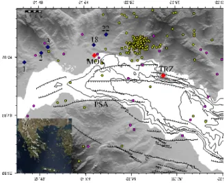
Figure 1.
Map of the western part of the gulf of Corinth (black square, left bottom insert) in Greece. Red diamonds : sites of bore-hole strainmeter (MOK) and dilatometer (TRIZ). Blue cir-cles : epicenters of 2010 Pyrgos earthquakes, M=5.3, ’18’: 18/01/2010 event, ’22’: 22/01/2010 event. Blue diamonds : epicenters of the 3 largest earthquakes in 2011, M=4 to 4.7, ’1’: 11/02/2011 event, ’2’: 07/08/2011 event, ’3’: 10/11/2011 event. Epicenters from the February swarm are plotted as yellow circles. Epicenters for julian day 339 (05/12) are represented by the purple circles (cf part. 4.3.). The scale (in kilometer) is representated on left top.In the attempt to detect and model strain transients in an ex-tensional tectonic context, strainmeters and continuous GPS have been installed in the western rift of Corinth, in Greece, within
the framework of the Corinth Rift Laboratory project (
http://
crlab.eu
). In particular, we installed twoSacks-Evertson
high resolution borehole strainmeters (Sacks et al. 1971): the rst in 2002, a Sacks-Evertson dilatometer, near the northern coast of the Gulf, on the Trizonia island; and the second in 2007, a 3-componentSacks-Everston
strainmeter, near the village of Monasteraki,10 km to the west (Fig.1). This high-resolution strain monitoring
complements the 5 continuous GPS (
https://gpscope.dt.
insu.cnrs.fr
) and the seismicity monitoring of the CRL arrays. In 2002, the Trizonia dilatometer has provided the rst record of a strain transient in the rift, lasting 30 minutes, associated with an unusually shallow (less than 3 km) M=3.5 earthquake on thePsathopyrgos fault system (PSA, Fig.1), which has been interpreted
as a slow creep event on the fault (Bernard et al. 2006). This tran-sient was part of a micro-seismic activation of the deepest part of this fault, which lasted 7 weeks starting mid-November 2002. The 10 years records from this dilatometer has been studied more ex-tensively by Canitano (2011), and will be the subject of a subse-quent paper.
In the present article, we focus on the Monasteraki strainmeter records, rst analyzed by Canitano (2011). After the presentation of the seismotectonic context of the western rift of Corinth, we describe the instrument and characterize some of its systematic,
spurious noise (steps and drift). We then report the strain sig-nal response to extersig-nal forcing (atmospheric pressure, oceanic loading), and to earth tide loading, which allows us to correct for these in uences. Finally, we present observation of strain induced by dynamic instabilities occuring after P and/or S waves arrivals. The present article is describing the in-situ calibration of a new-designed borehole strainmeter.
2. The seismic and tectonic context of the Western rift of Corinth
The rift of Corinth is an asymmetric graben, possibly the fastest continental rift on Earth (Armijo et al. 1996, Bernard et al. 2006), with measured geodetically extension varying from 5 to 15 mm/yr between the eastern and western ends (Briole et al. 2000, Aval-lone et al. 2004). The Corinth gulf is bounded by large, active E-W striking normal faults mostly outcropping near its southern coast, and dipping to the north (Armijo et al. 1996, Micarelli et al. 2003). In the western part of the rift, which is the focus of the present study, a set of recent en-echelon normal faults have connected the Psathopyrgos normal fault which marks the western end of the rift, to the Eastern Helike Fault (Palyvos et al. 2007, 2010). All these north dipping faults root near 5 to 7 km in depth within a highly microseismic layer (Lyon-Caen et al. 2004). The latter dips gently towards the north, and de nes a WNW-ESE active trend under the gulf. Some south-dipping, antithetic faults outcrop near the north-ern coast line, but most do not show any microseismic activity at shallow depth. The geometry of the microseismic structures is now accurately de ned thanks to the double-difference relocations of events recorded by the continous monitoring of the CRL-net seis-mic array, since 2000 (Lambotte et al. 2010).
The most recent signi cant earthquakes in the western rift are the Aigion (M=6.2, 1995) (Bernard et al. 1997), and the two 2010 Pyrgos earthquakes (both M=5.3) (Lyon-Caen et al. 2010). The former has activated a low dip angle, north-dipping, blind normal fault. The latter earthquake pair, around 6 to 8 km in depth, coincides with the northern edge of the micro-seismic layer, and may have acti-vated the root of the Psathopyrgos fault (Lyon-Caen et al. 2010). This fault has not ruptured historically (thus for at least 3 centuries) and presently has the potential for a magnitude 6.2, possibly up to 6.7 in case of a dynamic cascade linking neighbouring fault seg-ments (Bernard et al. 2010). Hence, the fault system in the west-ern rift of Corinth may be close to failure at the time scale of a few decades, which may explain its accelerated strain rate (reaching
10−6/year) and large seismicity rate (more than 10,000 events per
year).
The frequent and large seismic swarms of the western rift contrast with the steady strain rate deduced from continuous GPS, suggest-ing small, or even no aseismic deformation related to this seismic-ity, at the local resolution of GPS (equivalent moment magnitude M=5). However, owing to some diffusion characteristics of space-time evolution of the micro-seismicity, it has been proposed that these swarm events may be assisted or triggered by pore pressure
diffusion in the fractured, active layer (Bourouis and Bernard 2007), which remains to be quanti ed.
3. Description and qualification of the Monasteraki borehole strain-meter
3.1. The 3-component strainmeter of Monasteraki and complemen-tary measurements
The Monasteraki
Sacks-Evertson
3-component tensorstrain-meter (Sacks et al. 1971)has been installed at the end of 2006
(38.403◦N, 21.925◦E), 2 km west to the village of Monasteraki, on
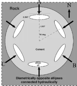
the northern coast, and about 350 m north to the shoreline (MOK site). The instrument, with sensing unit of 3 m long, has been de-signed and constructed by the Carnegie Institution of Washington. It is cemented at 150 meters depth in a borehole within the Trias-sic, fracturated sandstone of the Phyllade nappe. Coring and log-ging of the borehole has provided evidence, within the rock mass, of thin beds of sand, as well as of sand- lled fractures, which are expected to produce an heterogeneity which might a priori alter the sensitivity of the instruments (through anelastic relaxation of strain) and/or distort it (through an anisotropic elastic response to applied stress). The strain gauges consist of six steel elliptical tubes, 3 m long, each having large ellipticity, thus compliant to traction parallel to its smallest axis, and are lled with degassed uncom-pressible silicon oil. Diametrically opposite tubes are connected hydraulically to form a 3 component strainmeter. Volumetric strain of each gauge is transmitted through the oil to an LVDT sensor, whose output is proportional to the traction. The cylinders, with
vertical axis, are horizontally rotated by 120◦with respect to each
other, so that horizontal traction is measured in 3 directions
sep-arated by 120◦(Fig.2). This allows to resolve the horizontal stress
tensor variation (amplitude and orientation of principal stress). The data logger (SOC BOX) is continuously recording at 50 Hz the three
gauge signals (s1a, s1b, and s1c), with a resolution around 10−11at
short period, as well as air temperature and barometric pressure at 1 Hz.
We estimated the absolute orientation of the sensors by compar-ing the earth tide records to a theoretical model. The deformation
of the rock mass surrounding
ϵ
xxin a directionθ
(counted fromEast) normal to the gauge, due to the earth tide, can be linked to
Earth tidal strain by using the relation (1) (Jaeger and Cook 1976):
ϵ
xx= ϵ
eecos
2θ + 2ϵ
ensin
θ cos θ + ϵ
nnsin
2θ
(1)
where
ϵ
ee,ϵ
nnandϵ
enare respectively the east principalcompo-nent , the north principal compocompo-nent and the nord-east shear com-ponent of solid tide.
The theoretical components of earth tide tensor in equation (1)
are obtained by
ETERNA 3.3
(Wenzel 1995). The orientation ofeach strain component could then be estimated by the angle
θ
giv-ing the best waveform t between observed traction and theoret-ical solid strain combination. In the theorettheoret-ical tidal strain, we ne-glected the elastic deformation due to the Mediterranean sea tidal
Figure 2.
Representation of the MOK strainmeter orientation. Top view across the strainmeter and the borehole. Cylinders diametrically opposite are hydraulically connected, adding the effect of traction upon their surface. The gauge s1a (A) has an north azimuth direction and s1b (B) and s1c (C) are respectively 120◦CW and CCW from s1a (top view)..
loading (OTL), as it was shown to be about 80 to 100 times smaller than the elastic effect of the gulf tidal loading (Canitano 2011). Fur-ther, we restricted the data analysis to a few one week long periods , where the M2 signal was much less pronounced, in order to avoid the loading in uence of the nearby gulf at this tidal period. We
found optimal values of 0◦, 120◦, and 240◦from North, for the s1a,
s1b and s1c components, respectively, with an estimated
uncer-tainty of 10◦.
In complement to this recording system, down hole pore pressure in the borehole (cased down to 120 m) is monitored by a total pres-sure transducer (1 pt/10 mn) which provides water level after baro-metric correction. The gulf sea level is provided by the tide-gauge installed in the marina of the Trizonia island, located about 15 km east to Monasteraki.
3.2. Instrumental noise and drift on strain records
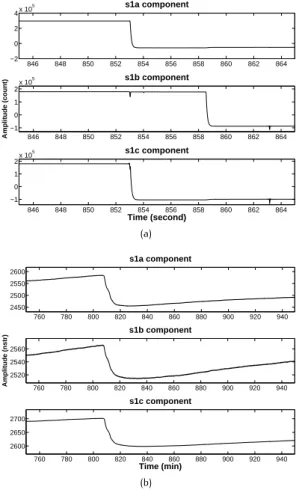
The recorded signal on each strain gauge often exhibits clear step-like signal, lasting less than a second, as shown by the rst signal
step on Fig.3(a). These signals are due to the valve opening when
the oil pressure becomes too high. The result is an extension on
each gauge with amplitude around 3.
10
5D.U for each component.Other kind of signals are strain signatures of small fracturing pro-cess close or in the immediate vicinity of one gauge causing a me-chanical stressing of the gauges by the rock. These signals could have a duration in the order of second to hour with strong ampli-tude, the strain shape on each component are linked to the
dimen-846 848 850 852 854 856 858 860 862 864 −2 0 2 4x 10 5 s1a component 846 848 850 852 854 856 858 860 862 864 −1 0 1 2 x 10⁵ s1b component Amplitude (count) 846 848 850 852 854 856 858 860 862 864 −1 0 1 2x 10 5 s1c component Time (second) (a) 760 780 800 820 840 860 880 900 920 940 2450 2500 2550 2600 s1a component 760 780 800 820 840 860 880 900 920 940 2520 2540 2560 s1b component Amplitude (nstr) 760 780 800 820 840 860 880 900 920 940 2600 2650 2700 s1c component Time (min) (b)
Figure 3.
(a) 20 seconds of MOK strain records (50 Hz sampling). The compression is positive and the amplitude is giving in count (D.U). The steps related to valves opening are ex-tensive with an amplitude around 3.105D.U for eachcom-ponent. (b) 3 hours of MOK strain records exhibing slow strain variations related to fracturing process close to the sensor. The amplitude is giving in nanostrain (see Table2
for calibration coefficients).
sions of the fracture and its position relative to each gauge (see
Fig.3(b)). This effect can affect one or more component.
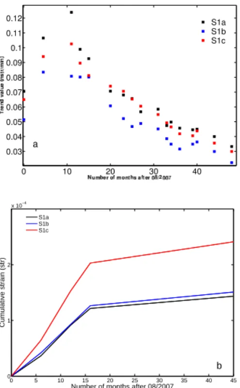
A second characteristics of the strain signal appears when we look
at longer data times series (Fig.4). Each strain component
ex-hibits a clear near linear trend. The analysis of the monthly drift indicates a fast increase of the trend value since august 2007 ( rst month where the instrument correctly operates), reaching a maxi-mum one year later. Then the trend is decreasing roughly linearly on each component (with equivalent values for s1a and s1c) dur-ing the last three years, and end of 2011 the values are divided by
three on each component (Fig.5(a)). This drift seems to be related
to a true mechanical effect of the surrounding rocks, and not to a sensor drift (LVDT), as the latter would not produce the reported inversion of drift rate nor the correlated drift between the three sensors. A possible explanation could be the progressive
tighten-Figure 4.
One month of MOK strain records on gauges s1a, s1b and s1c. The linear trend of each component is clearly visible, of the order of one tidal amplitude every day.ing of the borehole forced by the lithostatic pressure, which could be due to an initially weak coupling of sensor caused by improper cementation (as suggested by water ow in the borehole revealed by temperature logging). If we considerer the 150 meters of rocks above the instrument, the lithostatic pressure results in an
elas-tic areal strain around 10−4by assuming strandard rock properties
(
ν ∼
0.25,G
∼
30 GPa,ρ
sandstone∼ 2.5
). This value is the sameor-der of magnitude as the cumulative strain presently stored by each
component (Fig.5(b)). The small difference of cumulative strain
between the components could be related to a small heterogene-ity close to one gauge which could perturb the signal by shear or coupling variations due to uneven cementation.
3.3. Mechanical perturbations from external and internal sources: prediction and correction
Barometric pressure and gulf water level uctuations are the two major strain perturbation sources in Monasteraki. At longer peri-ods, days to months, the barometric pressure uctuation acts in combination with the mean gulf water level and both effects are correlated. Due to the absence of rain gauge, we could not take into account the compressive signal caused by surface or in ltrated rain onland, which may produce pressure at the time scale of hours to days of the order of few mbars. We do not consider either the elastic perturbation due to the OTL from the Mediterranean Sea located 80 kilometers west from Monasteraki, as already justi ed above.
As the instrument is not far from the gulf (350 meters), we tested for possible sensitivity of the gauges to pore pressure diffusion from the gulf due to sea level changes. This effect is indeed very strong on the Trizonia dilatometer, located 30 m away from the gulf (Can-itano 2011). For Monasteraki, a frequency band correlation be-tween the strain signal and the water level signal does not show a signi cant phase shift in the case of s1a and s1c. The s1b com-ponent shows a clear phase shift, which will be discussed later, but
0 5 10 15 20 25 30 35 40 45 0
1 2
x 10−4
Number of months after 08/2007
Cumulative strain (str)
S1a S1b S1c
b
Figure 5.
Strain rate (a) and cumulative strain (b) at MOK from 2007 to 2011. Components are identified by their color. The cumulative strain on each component can be related to the effect of lithostatic pressure due to the surrounding rocks.it remains relatively small. Thus, for simplicity of a rst order cor-rection, we considerer that the strainmeter is not sensitive to pore pressure diffusion effects from the sea, so that all the external forc-ing (sea level and atmospheric pressure) are actforc-ing instantaneously on the instrument. The only internal perturbation is the Earth tide strain, whose elastic deformation could be estimated by the
rela-tion (1) according to the gauge orientation.
The overall perturbation effects are considered to be elastic, thus they combine linearly. Therefore, the estimate of the induced strain related to each forcing is done through a direct correla-tion between each strain component and the three forcing sig-nals: solid tide, sea loading, atmospheric pressure. A spectral anal-ysis of each strain component reveals the semi-diurnal effect dom-inated by oceanic tides and the diurnal perturbation where solid
tide dominates (Fig.6(a)).
In addition to the perturbations above, the spectral densities ex-hibit clear signatures related to long period sea level perturbations. These are the mechanical effects of the free oscillations of the gulf (seiches) (Bernard et al. 2006). These oscillations with amplitude of a few centimeters are mostly triggered by wind. The s1c compo-nent seems to be less perturbed by this water mass loading, which can be explained by its orientation parallel to the coast, thus less sensitive to the expected dominantly NS traction related to local water load. The reference tide-gauge signal is recorded in Trizonia,
10−4.9 10−4.8 10−4.7 10−4.6 10−4.5 30 40 50 60 70 80 90 Frequency (Hz)
Power spectral density (dB)
s1a s1b s1c a 24 hrs 12 hrs 10−3.6 10−3.5 10−3.4 10−3.3 −10 0 10 20 30 40 Frequency (Hz)
Power spectral density (dB)
s1a s1b s1c
b
55 min 40 min
Figure 6.
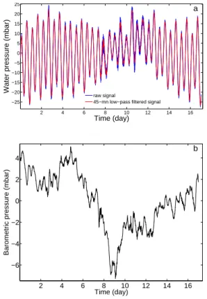
Power spectral densities of the strain components at MOK (color coded). (a) Zoom at low frequency on the diurnal and semi-diurnal frequency band. The related peaks of solid and oceanic tides dominate the spectra. The s1b and s1c components are 2 times more sensitive to 24-hours period tides than s1a whereas s1c seems to be a little less sensi-tive (1.5 times) to 12-hours period tides than the other com-ponents. (b) Zoom at periods smaller than 1 hour. Clear peaks appear at 50-55 min and at 38-40 min period, which are interpreted as the mechanical effects of the free oscil-lations of the gulf (seiches).thus 15 km from the site, so that at the period of the sea tide, the sea level at Trizonia and near Monasteraki can be considered to be in phase (Boudin 2004), and this still remains a good approxima-tion for the 50-55 minutes seiches. At higher frequencies, the 6-8 minutes seiche period recorded in Trizonia does not appear on the Monasteraki spectral records : therefore, a low-pass lter at 40mn period has been applied to the Trizonia tide gauge signal before
correlation with Monasteraki (Fig.6(b)).
The strain signals corrected from the linear trend and from the
the-oretical solid tide strain are presented in Fig.7, and the external
forcing (sea level and atmospheric pressure) are presented in Fig.8,
for june 2010. The correlation coefficients resulting from a linear combination between the three forcing signals and the strain
re-lated to each gauge are given in Tab.1. The coefficients resulting
from the analysis of a second period, 20 days long in December 2010, have been added in order to check the stability of the cor-relation, especially for the external forcing coupling which could be affected by a seasonal variability. The response coefficient to solid tide is stable for each gauge for the two periods, which is
2 4 6 8 10 12 14 16 −50 0 50 s1a component 2 4 6 8 10 12 14 16 −50 0 50 s1b component Amplitude (nstr) 2 4 6 8 10 12 14 16 −50 0 50 s1c component Time (day) a 2 4 6 8 10 12 14 16 −20 0 20 s1a azimuth 2 4 6 8 10 12 14 16 −20 0 20 s1b azimuth Theoretical strain (nstr) 2 4 6 8 10 12 14 16 −20 0 20 s1c azimuth Time (day) b
Figure 7.
17 days of strain records at MOK, june 2010. (a) Observed strain on each component corrected for the linear trend. The diurnal and semi-diurnal tide effects are clearly visible. (b) Solid tidal strain predicted for each gauge orientation (relation1). Note that this solid strain prediction shows a smaller semi-diurnal to diurnal ratio than the record, as the true record has a strong additional contribution from the local sea level at semi-diurnal periods.not surprising because the solid tide is the dominant effect in the strain signal especially at 24-hour period. The coefficient relative to the elastic effect of the sea level uctuation also seems to be quite steady. The stability of the barometric pressure coefficient is good in the case of s1a and s1b components, but seems to uctu-ate for s1c. This could be reluctu-ated to the stronger perturbations ob-served on s1c component, which perturbs the long period signal and hence the correlations with the non periodic in uence of the barometric pressure. Further analyis of the barometric presssure effect thus seems to be necessary especially in the case of gauge s1c.
The stability over time of the solid tide response coefficient allows us to give an accurate value for the solid calibration of each compo-nent. The calibration coefficient is simply the inverse of the tide
re-sponse factor (Tab.2).This coefficient combined with the response
coefficient to each external forcing provides the induced strain due
to this perturbations on each component (Table3). The induced
strain caused by gulf water pressure is twice smaller on s1c than in the other components, as a result of a less favourable orientation,
as illustrated by the spectral densities (Fig.6) seems to illustrate this
dependance. The spectral densities seems to argue in favor of a
2 4 6 8 10 12 14 16 −25 −20 −15 −10 −5 0 5 10 15 20 25 Time (day)
Water pressure (mbar)
raw signal
45−mn low−pass filtered signal
a 2 4 6 8 10 12 14 16 −6 −4 −2 0 2 4 Time (day)
Barometric pressure (mbar)
b
Figure 8.
17 days of external forcing at MOK, june 2010. (a) Sea level at Trizonia island: (blue) raw data; (red) low-pass filtered signal at 45 minutes period; (b) Barometric pressure fluc-tuation at MOK. Such signals are the forcing signals used for calibrating the gauges and for providing the calibration coefficients given by Table1.Table 1.
Gauge response coefficients. (CMS): solid tide (V/nstr),(CMA): gulf water pressure (V/mbar), (CPA): barometric
pres-sure (V/mbar). Gauge Period CMS CMA CPA s1a june 2010 49 81 366 dec 2010 43 83 390 s1b june 2010 52 50 353 dec 2010 57 57 348 s1c june 2010 57 56 559 dec 2010 60 47 385
stronger effect on s1b than on s1c which seems to be slightly the case. The s1a gauge also exhibits the stronger sensitivity to baro-metric pressure which may be explain by a horizontal anisotropy in response to surface load related to local elastic heterogeneity in the vicinity of the sensor.
Finally, the induced strain related to each forcing allows us to have a good prediction of the total induced strain, in agreement with
Table 2.
Calibration coefficient D′s1i(nstr/V) of a gauge i to internal deformation (solid tide).K′s1a Ks1b′ K′s1c
2,17.10−2±6.5% 1,83.10−2±4.5% 1,71.10−2±2.5%
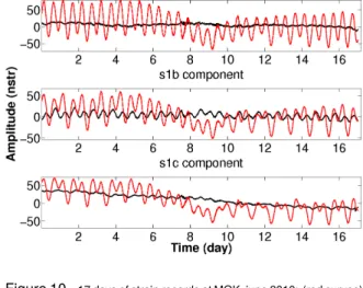
Figure 9.
17 days of strain records at MOK, june 2010: (red curves) detrended record of the strain on each component ; (black curves) total strain prediction obtained from the linear com-bination of the effect of the predicted solid tide and of the recorded sea level and barometric pressure, according to the correlation coefficients of table1.2010 are presented in Fig.9. The difference between the observed
strain signal and the predicted signal gives the residual strain
sig-nal for each gauge (Fig.10). The residual signals related to s1a and
s1c gauges are relatively free from external and internal perturba-tions. This is not the case for s1b component, for which a 12h-period signature persists, likely associated to unproper correction of the oceanic tides. This could be due to the combination of a pore pressure effect diffusion from the sea (thus out of phase with the sea level), with a partial uid coupling of the s1b gauge due to a defect in the cementation. Thus, to improve the overall reduction of external effects, in particular at 12 hours period, a frequency-dependence of the correlations should be conducted, especially for s1b. Such a correction was made for the Trizonia dilatome-ter (Canitano 2011),but for simplicity will not be considered in the present paper, as for Monasteraki it is a second order correction.
3.4. Quantification of noise in residual strain records
In order to quantify the correction above, we focussed on some period range with high energy: seiches at 50-55 min, tides in the 10-14h and 22-26h period range. In the domain of the long pe-riod seiches (50-55 min), the strain residual signals are at the level
of the instrumental noise (
∼ 10
−9), for each component (Fig.11).Figure 10.
17 days of strain records at MOK, june 2010: (red curves) detrended record of strain signal on each component; (black curves) residual strain signal obtained by the dif-ference between the observation and the prediction (see Fig.9). The s1b component exhibits a significant 12h-period residual, interpreted as resulting from a pore pres-sure diffusion from the nearby sea.Around 12h-period (Fig.12(a)) the correction applied on s1a and
s1c gauge allow us to eliminate respectively nearly 95% and 85% of the 12h-period perturbations, which is very satisfactory. The cor-rection performed on the s1b gauge is less efficient, as only 65-70%
of the perturbations could be removed. Around 24h-period (Fig.12
(b)), the correction results are similar to those obtained around 12h-period, except for s1c for which the correction is slightly bet-ter here (95%). As this diurnal period is dominated by solid tide, the quality of the correction at s1a and s1c seems to argues in favour of a good estimation of the solid tide. However, the stability of the phase delay between the residuals and the observations for each frequency domain, seems to indicate that the correction could be improved by taking into account a transfert function related to a simple pore pressure diffusion process from the sea.
A comparison between the strain signal related to each gauge and the water pressure uctuation measured on the top of the bore-hole does not exhibit any clear correlation for the s1a and s1c com-ponents around 12h-period (variable phase difference of the resid-ual). To the contrary, the s1b residual signal exhibits a clear corre-lation with the pore pressure signal at 12h-period (Canitano 2011), thus providing more evidence for the pore pressure diffusion from the sea to the borehole, as suggested above. This correlation may contribute to improve the correction for the forcing signals on s1b.
3.5. Implication of noise level for detection of slow sleep events
The residual noise level could be obtain by ltering the residual
strain signals (black curves in Fig.10) by the mean of a high-pass
lter. The noise level is considered, as a rst estimate, as the
Figure 11.
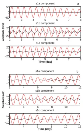
One day of residual strain signals during june 2010, in the 50-55mn period range: (black curves) residual sig-nal, (red curves) observed signal due to the seiche. The residual amplitude is of the order of∼ 10−9. The stabil-ity of the phase delays between the original records and the residuals can be explained by the a constant phase shift, due to the 14 km distance between the tide-gage in Trizonia and the coast line near MOK.2 3 4 5 6 7 8 −50 0 50 s1a component 2 3 4 5 6 7 8 −20 0 20 s1b component Amplitude (nstr) 3 4 5 6 7 8 −20 0 20 s1c component Time (day) a 2 4 6 8 10 12 −5 0 5 s1a component 2 4 6 8 10 −10 0 10 s1b component Amplitude (nstr) 4 6 8 10 12 −10 0 10 s1c component Time (day) b
Figure 12.
(a) 6 days of residual strain signals during june 2010 (black curves) and observed strain signal (red curves) fil-tered in 10-14h frequency band. (b) 10 days of residual strain signals during june 2010 (black curves) and ob-served strain signal (red curves) filtered in 22-26h fre-quency band.Table 3.
Induced strain on a gauge i caused by gulf water level fluctu-ation Gs1i(nstr/mbar) and by barometric pressure fluctuation Bs1i(nstr/mbar) retained in the present study.Gs1i Bs1i
s1a 1.78 8.2 s1b 0.98 6.4 s1c 0.86 6.6
Table 4.
Variation of the mean noise level (in nstrain) for s1a, s1b and s1c with dominant period of observation (high-passed signal in frequency).1h 5h 10h 1j 2j 5j
s1a 3 6 4 8 15 20
s1b 3.5 13 15 22 25 30
s1c 3 7 7 8 15 25
At very low period (around 1 hour, Fig.13(a)), the residual noise
level are the same order of magnitude for each component (around
10−9). When the period is increasing (around 10 hours, Fig.13(b)),
the level is around 5-7 nstrain on s1a and s1c and twice larger on s1b (pore pressure effect). At 2-days period, the noise level is about 15 nstrain on s1a and s1c and about 25 nstrain on s1b at 2-days
period (Fig.14). At 5-days period, the noise level is around 20-25
nstrain on s1a and s1c and around 30 nstrain on s1b. The instru-mental noise level increases with period, as suggested by Crescen-tini (CrescenCrescen-tini et al. 1997).
For qualifying the detection ability for slow earthquakes observa-tion, we assume a simple homogeneous half-space and a point
source dislocation with a typical normal fault dipping 40◦, and at
8 to 10 kilometers in depth. The elastic strain is calculated at the
instrument depth by using
COULOMB 3.3
, which is a revisitedversion of
COULOMB 3.1
(Toda et al. 2005), producing, asexam-ples, the following results.
If we consider the strain threshold to observe a signal as twice the noise level, an equivalent event of magnitude 5 at 5-days period should be detect on the three components up to a maximal dis-tance of about 15 km from the station. The two most sensitive components (s1a and s1c) should be able to detect a slow event of equivalent magnitude of 4 at 5-days period if it is located at a maximum of 3-4 km from the station. A slow event with same am-plitude occuring at 8-10 km should be detect by s1a and s1c up to 1-day period.
The analysis of the residual signals during the last years does not reveal any large transient event excepted a strong signal during December 2011, lasting 5 days with an amplitude around 60-70 nstrain, most probably related to a heavy rain episode. However, during the numerous seismic crisis occuring in the rift, the
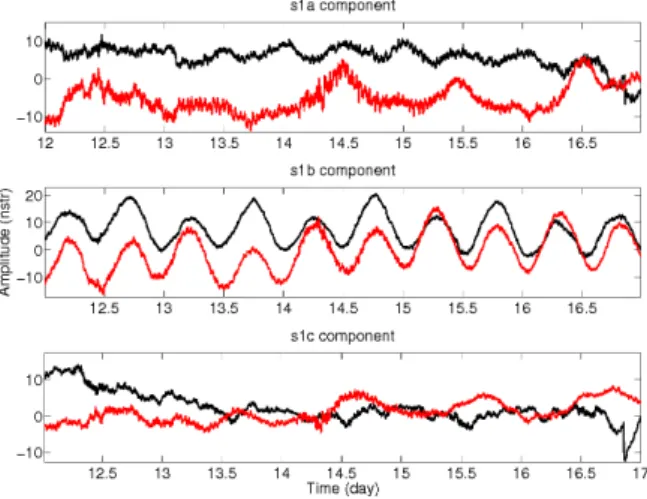
strain-87 88 89 90 91 92 93 94 95 96 −4 −2 0 2 4 6 s1a component 86 87 88 89 90 91 92 93 94 95 96 −10 0 10 s1b component Amplitude (nstr) 86 87 88 89 90 91 92 93 94 95 96 −5 0 5 s1c component Time (hr) a 300 310 320 330 340 350 360 370 380 390 −10 −5 0 5 s1a component 300 310 320 330 340 350 360 370 380 390 400 −10 0 10 s1b component Amplitude (nstr) 300 310 320 330 340 350 360 370 380 390 400 −5 0 5 s1c component Time (hr)
Figure 13.
Residual noise level (high-pass filtered) on two data sets (black (June 2010) and red (December 2010)). (a) 10 hours of signal at 1-hour period. (b) 4 days of signal at 10-hours period.meter sometimes exhibits small step signals, which are presented and discussed on the next part.
4. The 2011, 4-7 february seismic swarm
The western rift of Corinth has been quite active seismically during 2011. In addition to three earthquakes of magnitude greater than 4 in the northern part of the rift, ten kilometers west from
Monaster-aki, some important seismic swarms have occurred (Fig.15(a)). In
the following, we focus on a large, impulsive swarm, lasting three
days in February (Fig.1).
4.1. Step-like step responses
The beginning of february 2011 exhibits a high seismicity rate as
indicated by the hourly seismicity (Fig.15(b)). The related seismic
swarm is located about 5 km ENE to Monasteraki, and 5 kilometers
NW from Trizonia (Fig.1). The activity is mostly concentrated on
day 05/02 (day 36), at 5 to 8 km in depth, with epicenters clustered within 2 km. It occurred one or two kilometers east to the limit of the 22 January, 2010 Pyrgos earthquake rupture, and to its easter-most aftershocks. The strongest event had a magnitude 3.4 (05/02 at 02:52:38, NOA).
Figure 14.
5 days of residual noise level (high-pass filtered) at 2-days period on two data sets (black (June 2010) and red (December 2010)).During the three days of strong seismic activity, residual strain nals in Monasteraki are exhibiting numerous small step-like sig-nals, lasting less than a few seconds, with an amplitude of a few
nanostrain (Fig.16(a)). Almost all of this fast variations are
re-lated to seismic events associated to the swarm, as shown by the comparison between areal strain and vertical velocity compo-nent at Pyrgos short period seismic station, located just above the
hypocenter nest (Fig.16(b)). The largest strain variations seem
to be associated to the strongest events, but some large steps
are related to very small earthquakes (Fig.16(b), red line). The
areal strain (2/3 of the sum of the three components) shows a non-random time distribution of sign, implying sequences of compres-sional steps, lasting several hours, alternating with sequences of dilatation. Furthermore, when these steps are recorded on 2 or 3 components, they have the same sign (95% of the cases). We tested the hypothesis that these strain steps could be due to moment release of the coinciding seismic events, by rst assum-ing a mechanism similar to those of the nearby 2010 Pyrgos
earth-quakes (Fig.1). We calculated the volumetric and areal strain for a
source located at the center of the swarm, 6 km in depth, with an
EW striking normal fault mechanism (strike=280◦, dip=67◦,
rake=-90◦), using
COULOMB 3.3
(Toda et al. 2005). With a seismicmo-ment equivalent momo-ment magnitude around 4, we get an areal extension of 1 to 3 nstr in Monasteraki. Thus, in order to asso-ciate the reported strain steps to a source at the focus of the earth-quakes, the latter should have unusually large seismic moments with respect to their magnitude (between 1.5 and 3.5) deduced from their high frequency body wave radiation; alternatively, sec-ondary sources of strain could be located much closer to the instru-ment, being triggered at the passage of P and/or S waves. Unfortu-nately, no data could be used from the Trizonia dilatometer, which was stopped in the period mid-December 2010 to mid-February
35 35.5 36 36.5 37 37.5 38 2 4 6 8 10 12 14 16 18 Time (4−7 February, 2011) Seismicity (event/hr) b
Figure 15.
(a) Hourly seismicity during the year 2011 from the CRL-NET catalog. The red lines are indicating the 3 events with magnitude greater than 4 close to MOK. (b) Hourly seismicity during three days on february 2011 (4-7, days 35-38). The seismicity rate is dominated by a seismic swarm located about 8 km East of MOK (Figure1).2011. Thus, in order to test these alternative, we further analyzed the details of the coseismic strain, as follows.
4.2. High-frequency coseismic strain signals
We analyzed the 50 Hz records of the strain signals for more than 80 events (4 to 7 February), and found three main type of
wave-forms (Fig.17). The rst and most frequent type for all components
(60-70% of the events) is a step coinciding with the arrival of the rst P wave strain oscillation ; the step is completed in less than 0.5 s, so well before the S arrival about 1.5 s later. The second type (around 30% of the events) is a step coinciding with the rst S wave arrival. The last type, much less frequent, shows a ramp-like signal between the P and the S, stopping at the arrival of the S waves. In each case, the related strain values are in the range 1 to 3 nstr , with the same sign on each component for more than 95% of the cases. We also observed that only one strain event showed some step at the S arrival when it is observed at the P arrival (on s1c component), and none showed any ramp-like strain following the S wave. We investigated the degree of correlation between the peaks of the P and S, high frequency, oscillatory strain signals, with the type and amplitude of the low frequency strain step signal. We found that when the high frequency P peak strain value is the lowest (around 0.6-0.9 nstr for each component), the step coincides with the S
20005 2100 2200 2300 2400 2500 10 15 20 25 s1a component 2100 2200 2300 2400 2500 −5 0 5 10 s1b component Amplitude (nstr) 2100 2200 2300 2400 2500 0 1 2 3 s1c component Time (mn) a 2340 2360 2380 2400 2420 2440 4 6 8 10 areal strain Amplitude (nstr) 2320 2340 2360 2380 2400 2420 2440 2460 −5000 0 5000 10000
vertical component at PYR
Amplitude (V)
Time (mn)
b
Figure 16.
(a) 10 hours of residual strain signal at MOK during day 36, 2011 (5 February). The strain gauges are exhibiting some extensional or compressional steps with amplitude around 1-3 nstr. (b) 2.5 hours of comparison between the areal strain and the vertical velocity component at Pyr-gos (PYR) during day 36 (black square, figure (a)). The strain steps seem to be associated to the strongest seis-mic events during the crisis (Fig.1). One of them (around 2325 mn, red line) is unrelated to any relevant seismic wave.Figure 17.
Example of strain variation at MOK on s1b component during seismic episodes of day 36, 2011 (5 February): (a) step after P-wave arrivals, (b) step after S-wave arrivals, (c) gradual deformation between P and S waves. In each case, the related amplitudes are around 1-3 nstr.wave. For larger P-wave strain, the step is usually triggered by the P waves. But the step amplitudes do not appear to be simply cor-related to the high frequency wave amplitudes : P-wave induced
strain of 5.10−10could sometimes trigger a step with the same
am-plitude than a P vibration 10 times larger. For the strain gradual increase between P and S, they appear for small values of P-wave induced strain, close to the P-step threshold value.
We analyzed the coseismic strain signature for several events (about 15 events) from another swarm, in May-July 2009, located further way from Monasteraki, and found a similar typology, with similar amplitudes, and same sign 95% of the cases, suggesting the effect of secondary sources close to MOK.
A rst interpretation would be the activation of a small fault or frac-ture near the instrument, triggered by the P or S vibration above some strain threshold. When the P wave does not reach this thresh-old, the S wave would trigger the slip. Once triggered by P or S, the slip amplitude does not depend on the amplitude of the causative waves, but on the pre-stress and friction properties of the fault, which would explain the rather stable strain step amplitude. The non-random succession of compressional or dilatational steps, as well as the stability of the strain steps, suggests the existence of ei-ther a very limited number of such secondary faults , with a persis-tent mechanism, or several sources sharing a similar location and mechanisms.
Under the hypothesis above, the reported absence of successive P and S steps in the same event shows that the available sec-ondary sources are very few otherwise, for the same event, one source could provide a step on P, another one a step on S, and it would be statistically very unlikely that all would give the same response, at P or S arrival times. Then, if only a few secondary sources are active, these would have ruptured many times dur-ing the swarm sequence. Thus, as their faultdur-ing surface cannot be reloaded between successive slip events , they must be have a long-term, stored shear strain that they progressively release at each slip episode. But this seems in contradiction with the absence of S step following a P step : the slip triggered by the P wave is ex-pected to release a small fraction of the large available shear stress , thus one would expect that the following S wave could also trigger a second slip event. This last contradiction could be turned away by assuming an increase of the thresold level just after the slip due to the P waves, but no simple mechanism could support this ad hoc explanation.
Another intriguing observation is the equal sign (compression or dilatation) of the strain effect for all components in more than 90% of the cases, which strongly suggests a pore pressure effect close to the instrument, rather than slip on fractures induced by shear. Interestingly, the component with the smallest mean step ampli-tude, s1a, is also the less perturbed by the pore pressure diffusion from the sea, as seen previously: this suggests that a dominant cause for these steps would be pore pressure instabilities in loose cement or in sand pockets in contact with or close to each of the gauges.
Furthermore, this model would imply that when a slip event is re-lated to the P wave, it should produce a strain step on the three components of the instrument and similarly for the S steps. But this is not systematically observed. Furthermore, some P or S steps are mainly detected on one component : a null traction on two
di-rections separated by 120◦should occur very rarely, and requires
local heterogenity of the stress eld.
Thus, from all the arguments above, a model with unstable faults near the instrument, which would slip at the arrival of P or S waves, is not likely to be the dominant cause of the reported steps. We prefer a very local effect due to some non-elastic response of the immediate vicinity of each gauge, possibly due to slip on small frac-tures or cracks in the sandstone surrounding the gauges, or com-paction/dilatation within sand pockets or the cement itself, which could affect each gauge independently if they are at less than deci-metric scale. The small size of these sources of secondary strain would explain their limited impact of the signal. However, the way that such sources could show stable sign remains to be explained. To sum up this discussion for de ning the sources of these steps, we thus reject the dominance of effects from both the seismic fault at the hypocentral location, and secondary faults near the instru-ments (say within 1 m to 1 km distance), and favour a dominant ef-fect of instabilities in the immediate vicinity of the gauges (at less than 10 cm distance). This however does not exclude a direct elas-tic effect from the earthquake volume, for some of the rare step events unrelated with detected seismic shaking.
Over the three days of the swarm, the cumulated strain of the compressive steps is about 50 to 60 nstrain, and reaches a simi-lar value with the extensional steps, opposite in sign : this results in an cumulative strain change at MOK smaller than 10 nstrain for the whole sequence. In addition, at longer periods, the inspection of the 4 to 6 February strain signals show strain uctuation of less than 10 nstr, mostly due to uncorrected tidal effects at 12 hours pe-riod. The contribution of the elastic strain related to the direct ef-fect of the deep seismic and aseismic sources of the swarm is much smaller. If any transient creep episode associated with the swarm
had affected a 2 km
×
2 km fault within the swarm, the slip on itwould have been less than 40 millimeters.
Finally, we note that the largest earthquake of the sequence, which had a magnitude 3.4, produced an extensive areal strain step of 3.6 nstr. This value is still 10 times larger than the expected, coseismic elastic response, but very similar to the values of the spurious steps produced by signi cantly smaller events. This suggests the exis-tence of a saturation effect for the amplitude of the strain steps re-lated to the secondary sources near the instrument, which would allow a reliable retrieval of elastic strain steps for primary ampli-tudes larger than 10 nstr.
5. Discussion and conclusion
We showed above that the Monasteraki strainmeter, in the western rift of Corinth, can provide usefull, high resolution strain data for tracking slow strain transients, provided that care is taken to
cor-rect for several perturbating effects which will be discussed below .
The long term drift, presently showing a slowly decaying rate, can be removed from the records. Its amplitude is however still too
large (10−5/yr) for the local tectonic strain rate to be detected, - as
the latter is about 10 times smaller - if this tectonic elastic strain is not relaxed by anelastic strain and creeping faults in the shallow crust. We also note that the tectonics would promote interseismic extension at MOK, thus in opposite sign with the present compres-sive trend.
The sensitivity to atmospheric pressure has been evaluated at the dominant period of these signal, i.e around a few days assuming coefficient independant of frequency, which would be the case for a purely elastic shallow crust. If the latter has a non elastic be-haviour a long period through some relaxation process, then there should be a frequency dependence of the sensitivity. However the noise in the data does not allow to constrain this coefficient at pe-riods longer than a few weeks. Therefore, with the present data, we cannot exclude a long-term relaxation which could mask the tectonic loading effect, and/or slowly relax coseismic strain steps. The strain steps related to local instabilities on fractures limit our ability to accurately evaluate the coupling coefficients between the instrument and the atmospheric and sea level loading, in the ener-getic period range of weeks to months. The uncertainty on these coefficients is estimated to be 10-20%. Thus, this limits the accu-racy of the prediction of - and the correction for - the sea level ef-fect on the signal at the tidal diurnal and semi-diurnal periods. The progressive reduction in the yearly count of such steps, due to the stabilization of the borehole, may allow us to improve these cali-brations and corrections in the coming years. With the present cor-rection, at periods of days to several week or months, between the spurious steps, the residual of the correction from these in uences
has an rms less than 3.10−8.
The evidence for a pore pressure effect on gauge s1b, deduced in particular from a partial correction of the 12 hour sea tidal sig-nal, is interpreted as resulting from a partially decoupled contact of the gauge with the solid rock, due to a local cementation defect. This shows that there is a signi cant pore pressure diffusion pro-cess between the sea and the instrument, which should be taken into account for an improved calibration procedure, considering frequency dependent, complex correlation coefficients. This is ex-pected to further reduce the residual signal to probably less than 5% of the input signal, for all components. This unfortunately can-not be achieved yet, due to the remaining uncertainties on the sea loading coefficient, as explained above. Despite these problems, the diurnal and semi-diurnal effect of sea can be signi cantly re-moved from the records, with a remaining, uncorrected rms level
of 10−9and 4.10−10for s1a, 5.10−9and 1.5.10−9for s1b, and 10−9
and 8.10−10for s1c, at 12h and 24h-period respectively.
At shorter periods, the noise level is around 2-3.10−10in the
ab-sence of seismic activity. The detailed study of the 2011 February swarm shows that high frequency waves from local earthquakes
(M=1.5 to 3.5) produce coseismic strain steps (at P or S arrival times) in the range 1 to 3 nstr, much too large for resulting from standard, elastic coseismic changes. These steps are interpreted as due very local, secondary sources , possibly pore pressure instabilities, dy-namically triggered at the passage of the waves, located possibly within 10 cm of the gauges. A strong argument in favour of this model is that these steps are frequently recorded by only one or two of the three gauges. The amplitude of these steps is relatively independent of the amplitude of the triggering seismic wave,
pro-vided the latter is larger than about 5.10−10in peak strain. This
suggests that the small dimension of these triggered, secondary sources limits the maximal amplitude of the related strain: thus, one may expect that some coseismic strain signal larger than 10 nstr may not be dominantly caused by these local sources, and that such large strains should be related to the primary source, i.e., earthquake fault slip. This will be tested on the few available records of magnitude 4 events and will be subject of an other pub-lication.
Despite the unfavourable rock conditions around the sensor (frac-tured sandstones with sandy layers), the MOK station shows an un-expectedly good sensitivity to Earth tides, implying the ability to sustain medium-term elastic strain (several days), and a possibly rather limited non-linear response to local shaking implying the ability to respond elastically to the coseismic steps of the primary seismic sources.
After calibration and correction from the various external and in-ternal in uences, and despite the difficulties reported above, the Monasteraki strainmeter has provided preliminary but important informations on the transient process in this part of the rift of Corinth, for the period 2007 to 2011. First, no event similar to or larger than the december 3, 2002 strain transient has been recorded, despite the many large swarms within 20 km of the in-strument. The absence of such events is further con rmed by the analysis of the records of the Trizonia dilatometer (Canitano 2011), apart from the periods where both instruments were not recording (15-20% of the time since 2007).
The question of reliability of strain signals from borehole, high res-olution strainmeter, and of their contribution for seismic or strain transient analysis has motivated the present study. Our conclusion
is that the Monasteraki,
Sacks-Evertson
3-componentstrain-meter in the western rift of Corinth brings a very valuable contri-bution to the research on crustal transients, in an extensional envi-ronment, completing the continuous GPS monitoring and the Tri-zonia dilatometer. In particular, it reported no signi cant strain transient, even during seismic swarms. The resolution of the
instru-ment, of the order of a few 10−9at few hours and few 10−8at few
days, should be further improved in the coming years, through re-ned corrections from the external and internal in uences taking into account pore pressure diffusion from the sea. The apparent saturation of its weak, non-linear response to high frequency seis-mic waves, related to very local, dynaseis-mically triggered instabilities, should be further investigated. Finally, strain transient events, if
any, will be better tracked with the combined analysis of its mea-surements with those of the Trizonia dilatometer and of the future, strainmeters and tiltmeters planned in the area.
Acknowledgments
We thank the engineering team of the Carnegie Institution of Washington for providing, installing and maintaining the proto-type of 3 component strainmeter installed at MOK. We are grate-ful to Luca Crescentini for advising and validating oceanic tide cor-rections and commenting the preliminary version of this work. We also thank Nikos Germenis from the University of Patras for his con-tribution to the installation eld work. This work has been sup-ported by the EC/FP7 projects 3HAZ and REAKT the french ANR SISCOR contract and french INSU/CNRS for maintaining the CRL site. The Editor thanks the two anonymous reviewers for their as-sistance in evaluating this paper.
References
Armijo R., B. Meyer, G. C. P. King, A. Rigo, and D. Papanastassiou (1996), Quaternary evolution of the Corinth rift and its for the late cenozoic evolution of the Aegean. Geophys. J. Int. 126, 11–53.
Avallone A., P. Briole, A. Agatza-Balodimiou, H. Billiris, O. Charade, C. Mitsakaki, A. Nercessian, K. Papazissi, D. Paradissis, and G. Veis (2004), Analysis of eleven years of deformation measured by GPS in the Corinth Rift Laboratory area. C. R. Geoscience 336, 301–311.
Bernard P., P. Briole, B. Meyer, H. Lyon-Caen, J.-M. Gomez, C. Tiberi, C. Berge, R. Cattin, D. Hatzfeld, C. Lachet, B. Lebrun, A. Deschamps, F. Courboulex, C. Laroque, A. Rigo, D. Massonnet, P. Papadimitriou, J. Kassaras, D. Diagourtas, K. Makropoulos, G. Veis, E. Papazisi, C. Mitsakaki, V. Karakostas, P. Papadimitriou, D. Papanastassiou, G. Chouliaras, and G. Stavrakakis (1997), The Ms = 6.2, June 15, 1995 Aigion earthquake (Greece) : evidence for low angle normal faulting in the Corinth rift. Journal of Seismology 1, 131–150.
Bernard P., R. Charara, A. Serpetsidaki, P. Briole, and D. Diagourtas (2010), Embedded time scales of slip transients on the Psatopyrgos fault system, western rift of Corinth,Greece. ESC Meeting, Montpellier.
Bernard P., H. Lyon-Caen, P. Briole, A. Deschamps, F. Boudin, K. Makropoulos, P. Papadimitriou, F. Lemeille, G. Patau, H. Billiris, D. Paradissis, K. Papazissi, H. Castarède, O. Charade, A. Nercessian, A. Avallone, F. Pacchiani, J. Zahradnik, S. Sacks, and A. Linde (2006, October), Seismicity, deformation and seismic hazard in the western rift of Corinth : New insights from the Corinth Rift Laboratory (CRL). Tectonophysics 426, 7–30.
Boudin F. (2004), Développement d’un inclinomètre hy-drostatique à double niveau, et application au Golfe de Corinthe, Grèce. Ph. D. thesis, Institut de Physique du Globe, Paris.
Bourouis S. and P. Bernard (2007), Evidence for coupled seismic and aseismic fault slip during water injection in the geothermal site of Soultz (France), and implications for seis-mogenic transients. Geophys. J. Int. 169, 723–732.
Briole P., A. Rigo, H. Lyon-Caen, J. C. Ruegg, K. Papazissi, C. Mitsakaki, A. Balodimou, G. Veis, D. Hatzfeld, and A. De-schamps (2000), Active deformation of the Corinth rift, Greece : Results from repeated Global Positioning System surveys between 1990 and 1995. J. Geophys. Res. 105, 25605–25626. Canitano A. (2011), Analyse des in uences externes et in-ternes sur les mesures extensométriques en forage dans le rift de Corinthe (Grèce). Ph. D. thesis, Institut de Physique du Globe, Paris.
Crescentini L., A. Amoruso, G. Fiocco, and G. Visconti (1997), Installation of a high-sensitivity laser strainmeter in a tunnel in central Italy. Rev. Sci. Instru. 68, 887–905.
Ide S., G. C. Beroza, D. R. Shelly, and T. Uchide (2007), A scaling law for slow earthquakes. Nature 447, 76–79. Jaeger J. C. and N. G. W. Cook (1976), Fundamentals of Rock Mechanics. Halsted Press, New York.
Lambotte S., H. Lyon-Caen, P. Bernard, and A. Deschamps (2010), Microseismic activity and multiplets in the western part of the Corinth Rift (Greece). ESC Meeting, Montpellier. Linde A. T., M. T. Gladwin, M. J. S. Johnston, R. L. Gwyther, and R. G. Bilham (1996), A slow earthquake sequence on the San Andreas fault. Nature 383, 65–68.
Lyon-Caen H., P. Bernard, A. Deschamps, S. Lambotte, and P. Briole (2010), The January- February 2010 Pyrgos (western Corinth Rift) seismic swarm : a possible activation of the deep Psatopyrgos normal fault (Western Corinth Rift) ? ESC Meeting, Montpellier.
Lyon-Caen H., P. Papadimitriou, A. Deschamps, P. Bernard, K. Makropoulos, F. Pacchiani, and G. Patau (2004), First results of the CRLN seismic array in the western Corinth Gulf : ev-idence for old fault reactivation. C. R. Geoscience 336, 343–351. Micarelli L., I. Moretti, and J. M. Daniel (2003), Structural
properties of rift-related normal faults : the case of the Gulf of Corinth, Greece. Journal of Geodynamics 36, 275–303. Nadeau, R. M. and D. Dolenc (2005). Nonvolcanic tremors deep beneath the San Andreas Fault. Science 307, 389.
Obara K. (2002), Nonvolcanic deep tremor associated with subduction in southwest Japan. Science 296, 1679–1681. Obara K. and H. Hirose (2006), Non-volcanic deep low-frequency tremors accompanying slow slips in the southwest Japan subduction zone. Tectonophysics 417, 33–51.
Okada Y., K. Kasahara, S. Hori, K. Obara, S. Sekiguchi, H. Fujiwara, and A. Yamamoto (2004), Recent progress of seismic observation networks in Japan - Hi-net, F-net, K-NET and KiK-net. Earth Planets Space 56, xv–xxviii.
Palyvos N., M. Mancini, D. Sorel, F. Lemeille, D. Pantosti, R. Julia, M. Triantaphyllou, and P. M. De Martini (2010), Geo-morphological, stratigraphic and geochronological evidence of fast Pleistocene coastal uplift in the westernmost part of the Corinth Gulf Rift (Greece). Geological Journal 45, 78–104, DOI : 10.1002/gj.1171.
Palyvos N., D. Pantosti, L. Stamatopoulos, and P. M. De Martini (2007), Geomorphological reconnaissance of the Psathopyrgos and Rion-Patras fault zones (Achaia, NW Pelo-ponnesus). Bulletin of the Geological Society of Greece, 1586–1598.
Rogers G. and H. Dragert (2003), Episodic tremor and slip on the Cascadia subduction zone : The chatter of silent slip. Science 300, 1942–1943.
Sacks S., S. Suyehiro, D. W. Evertson, and Y. Yamagishi (1971), Sacks-Evertson strainmeter, its installation in Japan and some preliminary results concerning strain steps. Pap. Meteorol. Geophys. 22, 195–208.
Toda S., R. S. Stein, K. Richards-Dinger, and S. B. Bozkurt (2005), Forecasting the evolution of seismicity in southern California : animations built on earthquake stress transfer. J. Geophys. Res. 110, B05S16, doi :10.1029/2004JB003415. Wenzel H. (1995), The nanogal software :earth tide data processing package ETERNA 3.3. Bull. d’Inf. Marées Terr. 124, 9425–9439.