Applications of computers to balanced cross-sections

APPLICATIONS OF COMPUTERS TO BALANCED CROSS-SECTIONS

By

SARAH DAWN SALTZER

SUBMITTED TO THE DEPARTMENT OF

EARTH, ATMOSPHERIC AND PLANETARY SCIENCES IN PARTIAL FULFILLMENT OF THE

REQUIREMENTS FOR THE DEGREE OF

MASTER OF SCIENCE

at the

MASSACHUSETTS INSTITUTE OF TECHNOLOGY

MAY, 1986

@ Massachusetts Institute of Technology

Signature of Author

Department of EMarth, AtmospheTc and Planetary Sciences, May 9, 1986

Certified by

Kip Hodges Thesis Supervisor

Accepted by

Chairman, Department Committee on Graduate Students

WitHDPA .I ECH

Applications of Computers to Balanced Cross-Sections By

Sarah Dawn Saltzer

Submitted to the Department of Earth, Atmospheric and Planetary Sciences in partial fulfillment of the

degree of Master of Science at the Massachusetts Institute of Technology.

May 9, 1986

Abstract

Making the subsurface area of a geologic section balance is one technique aimed at helping the geologist determine the validity of a proposed deformed cross section. However,

checking for bed length balance in concentric fold regimes, area balance in regions of similar folding and finally

retrodeforming a section are all very time consuming steps. Using a series of four computer programs this entire

process can be simplified and the errors greatly reduced. The program SECTION uses topographic and structural orientation data to constrain the rough structural geometry along a line of section. Tests for balance can be made using the program BALANCE once the geologist has integrated his knowledge and interpretations with the computer generated cross section. The program BALANCE uses an iterative method for finally generating an area balanced cross section , a bed length balanced cross section, or both. This program also

retrodeforms, further constraining the validity of the section. A last pair of programs, THREEDIM and PROJECTION assist three-dimensional balancing of a volume of deformed strata.

This software package yielded successful results in the Canadian Rockies Front Range. Four cross sections were

interpreted independently from this area and were balanced and retrodeformed to test their validity. Using the data from these sections, two intermediate sections were created which passed all tests for balance.

Thesis Supervisor: Kip Hodges

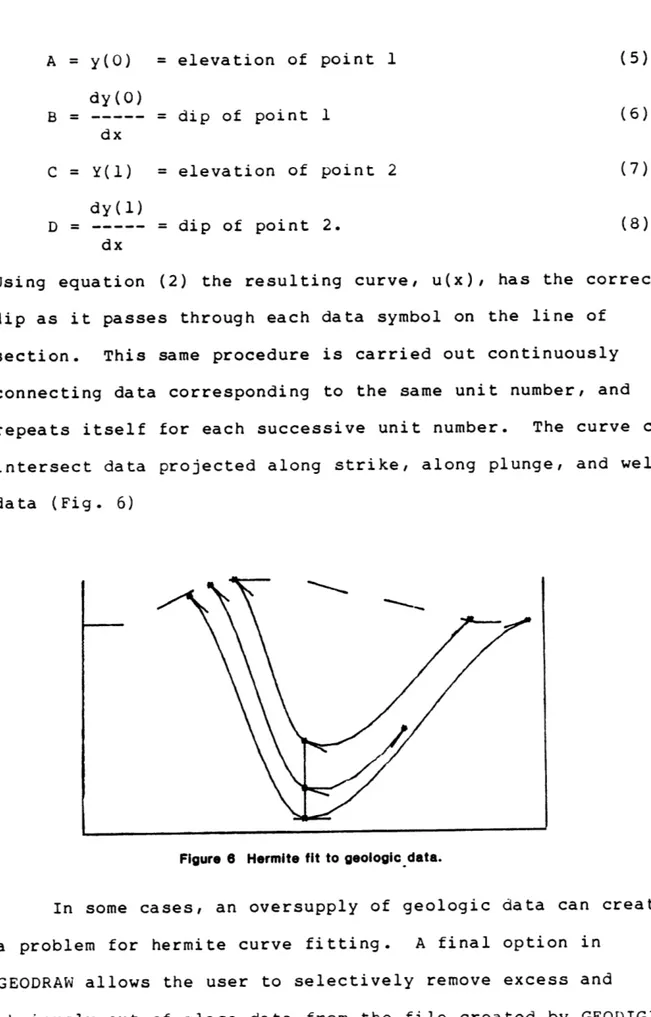
TABLE OF CONTENTS page Acknowledgements 4 Introduction 5 SECTION 8 BALANCE 22 THREEDIM 35 PROJECTION 39

Example from the Canadian Rockies 42

Conclusions 53

References 54

Appendix 1

SECTION and EXTRASUBS program listings 56

Appendix 2

BALANCE program listing 74

Appendix 3

THREEDIM program listing 90

Appendix 4

4

Acknowledgements

I would first like to thank Kip Hodges for being a wonderful thesis advisor, and having faith in my computer

programs when I had none. Peter Tilke has never stopped

helping and has had alot of input into the structure of these computer programs. Most of all, I would like to thank Dave Lineman for all of his time and effort in helping me survive the writing of this thesis and for being a great friend.

5

Introduction

The geologic cross section is a fundamental tool which permits the structural geologist to depict her or his

interpretation of subsurface geology. The permissibility of this interpretation can be examined by testing the cross

section for balance. The concept of balanced cross sections

was formally introduced by Dahlstrom (1969) and has since been

expanded upon by a variety of workers including Elliot (1983) and Woodward, Boyer and Suppe (1985). Strictly speaking, a

balanced cross section is one in which the two dimensional areas representing strata in the section are equal in area to

these strata in the undeformed state. Therefore, restricting cross sections to conform to a balanced geometry eliminates possible interpretations which do not adequately describe a series of events leading to a body of deformed rock

Cross section balancing, however, is a tedious task with many sources of error. In this paper I describe an

interactive software package which permits use of a desk top computer to streamline the balancing process, reduce the errors, and increase the reproducibility of interpretive sections. The initial programs assist the user in the

construction of preliminary sections from geologic data. The final programs permit the integration of several balanced sections from a single area into a three dimensional view of the structural style of the area

The programs are written in Hewlett Packard BASIC(2.l) for the HP 200 series personal computers. With minor changes, however, they can be altered to run on any computer system that supports BASIC. All of these programs require some sort of digitizing tablet for da.ta input. The digitizing and plotting commands assume a Hewlett Packard device which

supports HP Graphics Language (HPGL) for this purpose.

Therefore, lines in the program with these statements may have to be altered if different equipment is to be used. The

program BALANCE requires a RAM memory of one megabyte.

Finally, I have taken advantage of the soft-key feature of the HP personal computer in writing of the program SECTION. On the upper left hand corner of the keyboard there are ten keys of which eight are defined within the context of the program and correspond to different program segments. The need for these keys can be eliminated with GOTO and IF... .THEN

statements if user defined function keys do not exist on the keyboard of another system.

These four computer programs assist in all phases of cross section development and interpretation. The first program SECTION, assembles topographic, fold, well and structural data on to a line of section and makes a preliminary guess at the geometries. The next program,

BALANCE tests an interpretation for balance and then assists in attaining a balanced section. The Program THREEDIM

takes balanced cross sections from the same area and places them in a three dimensional grid defining the entire volume of

deformed rock. structures off

tne structures

The final program, PROJECTION, looks at

of the line of section and attempts to balance in three iimensions.

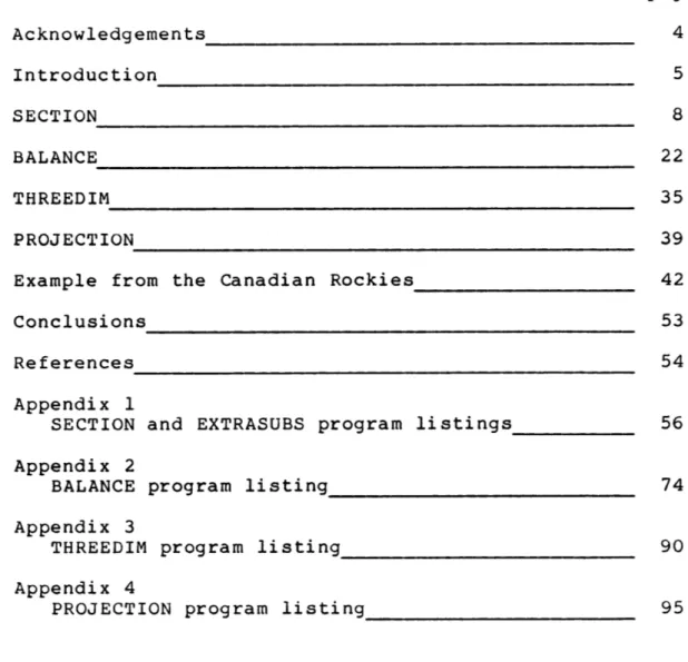
PROGRAM FLOW

01

01

-draw fodsn

-draw tooographic Profials -vroiect structural data

Are tre wany yes

more cros sectione *101m map area? Propct po to.*m Me 3-0 to new bw of section

"0

C-.0

_z

j>

SECTION

B

Caicuiate dowY?~pI5 projection A

(

SECTION

The first step in drawing balanced cross sections is to assemble all of the pertinent geologic data from the map and

to project it to the desired line of section. Then, from this skeletal section, the geologist can attempt to interpret the often complicated underlying structures. The program SECTION performs some of these more tedious tasks needed to create the base section, including generating topographic profiles,

plotting geologic data, and drawing folds.

The program is broken into sub-programs which call

various subroutines to pertorm some complex and often repeated functions. A few of these subroutines are stored in a

separate program, EXTRASUBS, and are independently loaded and deleted as they are needed by a program segment. When a given program option is completed, the user returns to the primary command level of the program with the option of choosing another branch defined by a different soft-key.

Getting Started

The computer needs some basic information in order to do any calculations and manipulations. At the start of the

program the user must input the scale of the map. The

orientation of the line of section is extremely important and the two endpoints must be input (digitized on the plotter). The map should be oriented on the plotter with north pointed to the top of the plotter. All output that is generated will be at the same scale as the original map in metric units.

TOPODIGIT

This program segment digitizes the topography for the construction of a topographic profile. The user first inputs

the elevation of each point which is to be digitized along the line of section. Given that most Canadian and USGS topo maps do not have elevations printed in metric, these numbers can be input in American Standard Units (feet) and will be converted internally.

The user next digitizes, from left to right, each data point along the line of section. The program rotates the line of section to be parallel with the base of the plotter and

then automatically creates a binary data file containing these data on the current floppy disk. The user inputs a file name and the file that is generated has the word "Topo"

concantenated to it. This file will be used by the next program segment, TOPODRAW.

TOPODRAW

There are two options available for drawing topographic profiles. The computer can simply "connect the dots" (the elevation data points) or instead can fit a cubic spline curve, Strang (1985). In either case, the computer concludes by drawing the vertical axis and labelling the high and low elevation in meters (Fig. 3).

The cubic spline fit uses the subroutine SPLINE which is automatically loaded from the batch of extra subroutines. A cubic spline interpolation is exact and the curve is

12 970 meters -- --- 790 meters -970 meters ---- 790 meters

Figure 3 comparison of straight line fit and cubic spline fit.

The first part of the cubic spline routine calculates a

best fit slope at each point for the curve. For a set of x-coordindate points XO... XN and corresponding elevations YO

.... YN, the best slopes SO....SN are determined by the matrix

equation: As=B (1) where, _s=SO*--SN and,-2 1 Y -YO Hi H₁ Hl2 1 2 + 2 1 Y3-Y7 t Y7-Y A= H₁ H₂ H₁, H2 B H3 H2 1 2 YN-YN-l HN HN _HN

The variable H is the spacing between the x-coordinate values

where Hi=Xi-X₀, H2=X2-Xi, .... ,HN=XN-XN-1- Once the slopes

have been determined, a hermite fit, Strang (1985), is used to calculate the curve connecting the points with known slopes.

A hermite curve fit simply connects two points each with known elevation and slope. Unit distance between points is assumed and the resulting curve is scaled at a later time. The curve is calculated using the equation:

u(x)=A(x-1)2_{(2x+l) + B(x-1)}2_{x + Cx}2_{(3-2x) + Dx}2_{(x-l) (2)}

where, A=Y₀ B=S₀ C=Yl D=Sl,

and the resulting curve is fit between the first two points. This procedure is then repeated for points 2 through N. The result is a smooth curve passing through the center of each topographic elevation point.

FOLDDIGIT

The program segment FOLDDIGIT enables the user to produce vertical or axial down-plunge projections of a fold outcrop. The user marks a number of points along the contact of a

folded layer at its intersection with the topography. Next the user enters the elevation of each of these data points, in metric or in feet, and then proceeds to digitize each point along the outcropping contact. All of this information is stored in a file with "Fold" concantenated to the file name,

AXIAL

Technically, one would not put an axial projection on to a cross section. However, the down plunge view can be

interesting to the geologist in order to classify the types of folding within the region. An axial projection is a view of

the fold across a plane which is perpendicular to the plunge vector in space.

The program segment AXIAL reads a data file created by FOLDDIGIT and projects each point individually along a user input plunge and trend onto a plane normal to the plunge

vector. After viewing the projection, the user has the option of choosing a slightly different plunge and trend, if these values are not well constrained.

The user next connects the projected data points defining the down plunge projection via short straight line segments or by the use of a best-fit polynomial The best fit polynomial curve is obtained with the use of the subroutines POLY and

INTERVAL which are automatically loaded from EXTRASUBS. INTERVAL redefines the location of each point along the x-axis. The accuracy of each point location is slightly reduced as the x-value is rounded to two significant figures where the fractional value is a multiple of 0.25. The purpose of INTERVAL is to redefine each point so that the final

polynomial, which is drawn at intervals of 0.25 plotter units

(1/16 of an inch) will actually pass through each point

exactly.

Once the points have been redefined, the subroutine POLY determines the best fit polynomial. POLY uses x and y

coordinate values obtained from INTERVAL and renames them WW(*) and UU(*) respectively. The user inputs a suggested order for the polynomial which can be easily changed if the resulting curve is unsatisfactory. A polynomial of order n has

the form:

y = ao+aix+a₂x2+a₃X3+...+anxn (3)

where x goes from the minimum value of UU(*) to the maximum value of UU(*) and y corresponds to the resulting WW(*) between these 2 endpoints. The constants ao through an are

16

best determined in a least-squares sense by the relation:

ATAC = ATB (4) where, 1x₁ n-i 1 xo . . . x0n- an-1 YO 1x . . . x1 n-1 an-2 Yl A=. C = . B =. n-i - -1xm-- - - m-1 a₀ Ym-1

for a set of m distinct points. The final curve contains points spaced every 1/16 cm which are connected by straight line segments (Fig. 4).

FOLDDRAW

This program segment accesses the same file used by AXIAL to create a vertical view of the fold along a user input line of section. The points are projected along their plunge

vector in space to, the intersection of this vector with a vertical plane containing the cross section (Fig. 5).

Finally, the data points can be connected by straight line segments or a polynomial best fit curve, as described in the last section.

17

4A' 10 "A

A' 1389M

A

851 M85 M

Figure 5 Vertical projection using FOLDDRAW.

GEODIGIT

This procedure assembles files containing the locations

and the values of a number of geologic data points. The geologic information can be: 1) strike and dip measurements

to.be projected along strike to the line of section; 2) strike and dip measurments to be projected along the plunge and trend

of the surrounding structure to the line of section; 3) or well locations. The information for each of these three data types is input in a slightly differing manner.

For strikes and dips projected along strike to the line of section, the user inputs both the strike in degrees from north and also the direction, east or west. Dip is input in the same manner and the location of the symbol on the map is digitized. These data are stored in a binary data file with "Geo" concantenated to the user input file name . These data are then projected by the program segment GEODRAW to the

appropriate x-coordinate position along the line of section and are plotted on the resulting section showing now the apparent dip at the elevation of the topography at that same

x-coordinate position. If The computer also asks for the unit number. Each stratigraphic unit should be assigned a number so that contacts may be fit to the data.

If the rocks in the location of these same symbols are involved in large scale folding then as an alternative the projection can occur along the regional trend and plunge of

the underlying structure. In this case, the strike, dip, and unit number are entered as before, and then in addition the user inputs the regional trend measured in degrees from north,

the direction E or W, and the plunge and plunge direction

measured in the same manner. The user next digitizes the

location of the strike and dip symbol on the map and all of the above information is then stored sequentially in the same "Geo" file. When these points are eventually drawn onto the line of section by the procedure GEODRAW, they are projected along trend, down plunge, and plotted at their resulting elevation with their apparent dip.

For well locations, the user inputs only the general strike of the beds and then digitizes the location of the well on the map. The file containing all well information is created separately using the procedure WELLFILE1.

WELLFILE1

This program option is used only in conjunction with GEODIGIT and basically creates binary data files with "Well" concantenated to the file name, containing well information. For each unit or contact encountered in the well for which there is information the user enters the depth, the general dip and dip direction and the unit number in order of

increasing depth. Wells are projected horizontally along strike to the line of section and are drawn onto the cross

section so that the depths of units correspond to the same scale as the topographic elevations.

GEODRAW

In order to actually invoke this program segment the user must choose option 8 from the main command level, "Draw Cross

Section". This procedure will itself call GEODRAW as it is needed.

GEODRAW goes a step beyond plotting geologic dip symbols on a cross section correctly. It can also draw hermitian

curves to fit the data by invoking the subroutine HERMITE. A hermite cubic finds the best fitting curve to two points when

for each point the y-coordinate (elevation) and the slope (in

this case, apparent dip dy/dx) are known. This corresponds to:

A = y(O) = elevation of point 1 (5) dy(O)

B = --- = dip of point 1 (6)

dx

C = Y(l) = elevation of point 2 (7) dy(l)

D = -= dip of point 2. (8)

dx

Using equation (2) the resulting curve, u(x), has the correct dip as it passes through each data symbol on the line of

section. This same procedure is carried out continuously connecting data corresponding to the same unit number, and repeats itself for each successive unit number. The curve can intersect data projected along strike, along plunge, and well data (Fig. 6)

Figure 6 Hermite fit to geologic data.

In some cases, an oversupply of geologic data can create a problem for hermite curve fitting. A final option in

GEODRAW allows the user to selectively remove excess and

obviously out of place data from the file created by GEODIGIT or WELLFILL1 so that a curve can nicely fit the data.

Draw Cross Section

This procedure enables the user to combine two or more types of output onto one line of section. This reduces to superimposing topographic and geologic data together, or topographic and fold data together on to one line of section. With fold and topographic data this is quite

straightforward. The fold is drawn to intersect the

topography at the same x-coordinate position and elevation on the cross section as on the map. The merging of topographic and geologic data is much more involved .

Certain geologic data, for example symbols which are projected along strike, are plotted at their resulting

x-coordinate position and at the elevation of the topography at that point. Therefore, the computer must already have the

necessary topographic information to plot the point

correctly. Once all of the symbols have been placed on the line of section by invoking the abilities of GEODRAW a

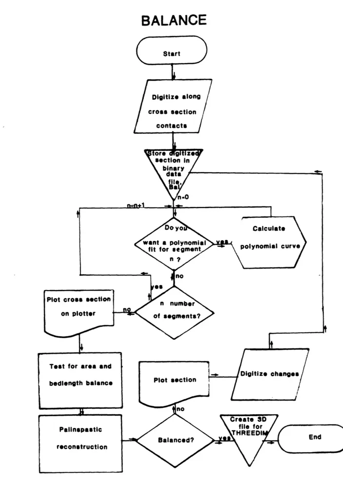
BALANCE

BALANCE

The program BALANCE uses a succession of methods to determine whether geologic cross sections can be defined as

balanced. The input for this program consists of digitized cross sections drawn by the geologist. After a preliminary test for balance, using an iterative approach, the user can simply dictate a change in the cross section to successively converge on a cross section that is either area or bed length balanced. Files of data are maintained and updated for

reproduction purposes.

The first step in checking for balance is to digitize a cross section which has been drawn using accurate geologic data from a map. The computer can handle data for up to 4 layers and 8 faults. The data arrays are easily redimensioned if extra memory is available. The user inputs the scale of the section and the name for the output file containing the digitized cross section information. Initially, up to 20 points are digitized along each fault from left to right, starting at the left-most fault. The last point is digitized twice to inform the computer of the fault end. After all of the faults have been digitized, the x and y location

coordinate values for each point are stored in a

separate file from the layer contact information, with II concantenated to the file name.

Next, the layer contacts are digitized starting on the left side of the cross section. The user digitizes individual

points along a path defined by the contact boundary. When either a fault or end of a layer is encountered, the point is digitized twice. A "segment", which is defined as a contact bounded by 2 faults or a fault and the end of the cross

section can have up to 25 points digitized along it. A

separate binary data file with "Bal" concantenated to the file name is created.

If mistakes are made while digitizing, and are recognized early enough, they can be corrected. If a point along the middle of a segment is digitized twice and yet does not border along a fault, pressing the number (3) clears the second

digitized location. In addition, because a file is created once the faults are all digitized correctly, if a serious

error occurs subsequently in digitizing along the contacts and it is necessary to start over, then the faults do not have to be redigitized if the location of the cross section on the plotter has not changed. The user simply reactivates the program, inputs the same file name, and enters zero (0) for

the number of faults. Digitizing Techniques

This program assumes that all faults cut all bed contacts and all layers. In some casesfor example blind thrusts

(Boyer and Elliot, 1983) this criterion is not satisfied. However, simple digitizing techniques can allow for more

complicated sections to be tested for balance. In the case of blind faults, simply extending the fault with no displacement

into the upper layers can solve the problem.

Another problematic situtation arises when sections contain horse structures, created when imbricate thrusts propagating in front of earlier thrusts, finally rejoin the earlier thrust. Some layer contacts may not exist within a horse bounded by 2 faults. To solve this problem, the user digitizes consecutively along the contact in question,

digitizes twice at the first fault, digitizes one imaginary point 2 times within the horse structure and then continues digitizing immediately to the right of the second bounding

fault. Finally, overturned beds create a problem for polynomial curve fitting. One solution is to draw an

imaginary fault with no displacement along the axial plane of the fold. The result will be to divide the bed into two

segments for separate curve fitting. Polynomial curves

After all digitizing has been completed, polynomial functions can be fit to the individual segments which were defined earlier. The object of the polynomials is to obtain

detailed shapes of beds so that the computer can have more accurate information for balancing calculations.

When a cross section containing only a simple fold is digitized and calculations are performed without a polynomial

fit the bedlength is calculated by summing the straight line segments defining the fold between the digitized points. The errors associated with this procedure can be noticeable. In

perfectly cyclindrical folds, for example, with a radius of curvature of 100 m and digitized points spaced every 100 m the error is 2.7%. Clearly, if spacing between digitized points is decreased, then the accuracy of calculations increases in both bed length and area balanced sections. This is the basis for the polynomial fit.

The program, BALANCE calls the same subroutine, POLY which was described in the program SECTION. Polynomials for each segment can be up to 8th order, yet must have an order

less than or equal to the number of points in the segment. The user decides for which segments polynomial fits may aid, and may settle for the straight line fits in unfolded regions in

order to save time. The digitized points within the segment are projected onto the CRT so that the user can choose an

appropriate order for the resulting polynomial. If the fit is not adequate, the process can be repeated a number of times to satisfy the user. Polynomial fits are also calculated for the faults.

The polynomial curve which is generated is not actually a curve, but rather a collection of short connected line

segments, each segment being 1/16 cm long in the x-direction. The result appears as a continuous curve. If folds have been digitized with care, for example hinge and trough points have been entered as well as more points in zones of increased complexity (inflexion zones), then polynomial curves can

27

After polynomial curves have been fit to the desired sections, the entire cross section can be plotted on the CRT or on the plotter. It is generally a good practice to view

the section as a check for digitizing errors. Tests for Area Balance

In many foreland fold and thrust belts the deformation path is approximately plane strain. Therefore, one can orient

the section parallel to the transport direction so that

conservation of rock volume becomes conservation of area in cross section. _{The bed area in a deformed cross section must} equal the area in the undeformed state for a section to be acceptably balanced.

The general method of the area balance procedure is to integrate to find the entire area below the highest contact down to the bottom of the cross section. This procedure is repeated to find the area under the next lower contact. By subtracting these 2 quantities, the area of the bed layer in

cross section can be determined (Fig. 8).

Layer area=

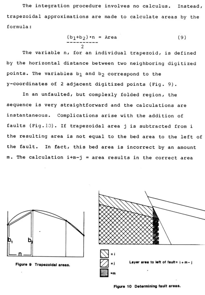
The integration procedure involves no calculus. Instead, trapezoidal approximations are made to calculate areas by the formula:

(bi+b₂)-n = Area ₍₉₎

2

The variable n, for an individual trapezoid, is defined

by the horizontal distance between two neighboring digitized points. The variables bi and b₂ correspond to the

y-coordinates of 2 adjacent digitized points (Fig. 9). In an unfaulted, but complexly folded region, the sequence is very straightforward and the calculations are instantaneous. Complications arise with the addition of faults (Fig.10). If trapezoidal area

j

the resulting area is not equal to the bed area to the left of the fault. _{In fact, this bed area is incorrect by an amount} m. The calculation i+m-j = area results in the correct area

b,

Figure 9 Trapezoidal areas. a Layer area to left of fault= 1+ m- J

am

29

determination. Therefore, the variable m must be calculated in order to obtain the correct bed area value. m is simply a trapezoidal area with bl and b2 defined by the value of the intersection of each of the contacts with the fault surface.

A similar calculation must be made to the right side of the

fault, yet m (which has a different value here) is subtracted. When faults are curved and are fit by polynomials the value m is simply the sum of many small areas.

Sub-areas for individual sections are next summed up across faults and discontinuities to determine the total area

per bed within the cross section. Since we assume that the

area of this bed remains constant before and after

deformation, then, the original, undeformed length can be determined by relation (9) if the undeformed thickness of the

bed is known. The value of the original thickness of the bed can be input by the user or digitized off of the plotter. The value for scale, input at the start of the program influences the technique to be used. If the true thickness of the bed is well constrained, the user should input the actual scale of the cross section at the start of the program and the

undeformed length in relevant units and correct scale will be output. If the original bed thicknesses are not well

constrained then the user can digitize the thickness of the layers directly from the cross section. Each layer thickness can be digitized a few times across the section to obtain an

30

average thickness. Using this method, the scale input at the start of the program should be 1. The resulting output will be in real units relative to the digitized cross section.

The geologist must judge whether a cross section is

balanced by examining and comparing the computer generated pre-deformational bed lengths. The computer calculates the mean bed length and the standard deviation. The final error analysis compares the maximum bed length difference to the mean bed length. Ideally, all bedlengths should be exactly equal, or some plausible explanation should exist for a

deviant bed. However, in a perfectly balanced section, slight digitizing errors can result in minor area errors. Woodward et al. (1985) discuss this phenomenon in detail. The computer allows for the user to change the thickness slightly to attain perfect balance. The computer calculates the standard

deviation of the bed lengths and also a percent confidence. My experience shows that standard deviations in balanced sections with a scale of one should lie in the 10-5 range. The percent confidence uses the calculation:

%confidence = maximum bed length - minimun bed length

--- X 100 mean bed length

(10) the values of %confidence should be greater than 97% to

31

Bed length Balance

Sections which exhibit area balance may be tested for bed

length balance as well if the folding is concentric. In

regions of similar folding bed length balance is inappropriate

because the length of a layer before and after similar folding does not remain constant. Bed length balance requires

significantly fewer calculations and has a lower probability of error.

This routine sums up the distances of the individual straight line segments connecting digitized points by segment for an entire curved contact offset by faults. If the curve has been fit by a polynomial then a large number of

significantly shorter segments are summed with a more

accurate result. Individual bed lengths

should be equal. In addition, as a final check, the bedlength balance technique should yield a mean length with a value

similar to the mean length determined in the area balance routine.

Tests for bedlength balance generate values for strain as well for each contact length. Strain (e) is calculated

independently with the formula:

L-LO ₍₁₁₎

Lo

where L is the length of the deformed bed in cross section, and Lo is the unfolded and unfaulted length.

32

Palinspastic Reconstruction

Retrodeforming a cross section is a final

technique used to balance cross sections. The palinspastic reconstruction is basically a view of the undisturbed

stratigraphic wedge with the predeformational insipient fault geometries sketched in. Cross sections which are not balanced

will contain fault surfaces which do not adequately describe a deformation path, showing vertical faults and faults showing an incorrect dip.

The retrodeforming procedure in the program BALANCE first draws out the flat stratigraphic wedge using the lengths and

thicknesses calculated earlier. For viewing purposes, the

mean length may be plotted for all beds. Any cross sections which are retrodeformed must already exhibit area balance or

the retrodeformation is meaningless. Faults are drawn in

assuming that the bed area between two faults remains constant before and after deformation. This is the only requirement affecting the resulting geometry of the reconstructed wedge.

Relative contact lengths between faults are not taken into account nor is the deformed fault shape or hanging wall and foot wall cutoff lengths. These "sub-areas" are calculated for each layer between each fault and the computer calculates each "sub-length" using relation (9). If rectangles

containing the correct areas are plotted, the result could by stepping faults (Fig. 1la). Instead, to give the fault a

curved surface, a polynomial function is fit which goes through a

33 a) b)

I:.

Figure 11 Refer to text.

point on each layer halfway through the thickness of each

layer at the edge of the rectangle (Fig. 11b). The user should choose polynomials of order 3 or 4 depending on the number of strata in the wedge.

The resulting palinspastic reconstruction (Fig. lic) must be further interpreted by the user. Fault surfaces must be extented to the top and bottom of the wedge, and in some cases the curvature must be reduced(Fig. lid). In addition, the user must selectively rule out and redraw some surfaces as the

computer may not have enough information to draw the correct surface.

Redigitizing Sections

Most cross sections, after a first check do not pass the requirements for area balance. As a result, subtle changes

are generally needed to obtain balance. This computer

program interacts with the user to obtain satisfactory changes in the cross section configuration.

If changes are desired, the entire cross section is drawn onto the plotter with the location of every point which was originally digitized by the user starred and numbered. These digitized points can be moved, one at a time to change the bed

shape. In addition, points can be added. The user in this case enters the location numbers of the points to the left and

right of the location for the new point, then digitizes the point. After a single change has occurred, the cross section may be redrawn and renumbered. This is especially useful if

points have been added, as the numbering sequence changes slightly.

When cross section changes have been completed, binary data files are updated to reflect the changes and renewed tests for balance can occur. The procedure must be entirely reactivated starting with fitting polynomials to sections.

35

THREEDIM

Digitize location

of this section/

on plotter

Figure 12 Flowchart for THREEDIM.

Locate inflection points Place digitized points in grid Digitize structural features

36

THREEDIM

The main object of the program THREEDIM is to set up a three-dimensional grid defining a volume of deformed rock. The geologic map forms the 2-D base of this grid and the vertical cross sections, in their proper positions along the map create the third dimension in space. In this way, the relationships between a number of cross sections can be interpreted and the implications for intermediate cross

sections can be examined.

The grid itself does not contain complete cross

sections. Instead, the user chooses key points on the cross section which can aid eventually in the construction of

other intermediate sections. The next program, PROJECTION, takes these points and projects them along structural trend and plunge to desired cross section locations. These key markers should include hinge and trough locations,

inflection points,. and hanging wall and footwall cutoffs at fault boundaries.

Therefore, the user must initially compile a list of "projectable" points from all of the cross sections on the map. This list should include key points common to all

cross sections in addition to key points on only one or more sections. This entire list must be entered, in the same order, each time THREEDIM is re-run for a cross section from

this map. This process helps to avoid data confusion later on as THREEDIM is re-run for successive cross sections. The next step is to digitize the location of one section on

37

the map to be included in the grid. Because this program is rerun for each cross section, the location of the map on the plotter cannot change or future projections will be

incorrect.

A binary data file containing x and y coordinate values of every point on the cross section is next read by the

computer and the geologic cross section is projected on to the CRT display. This file must have previously been created by the program BALANCE. It is assumed that any cross sections placed in the grid have been tested successfully for balance.

There are two types of files which can be retrieved in this step. The simplest file contains only points which were digitized off of the original cross section. This file which has "Bal" concantenated to the file name was created and

modified by BALANCE and is intended basically for use with that program, yet is sufficient for use here if folding is minimal. As an alternative, and a necessity in complexly

folded regions, a file containing polynomial fits to the data may be used. This file with "Poly" appended to the name was created by BALANCE near the end of the program for specific use by THREEDIM.

With a given cross section in full view, the geologist can selectively choose those aspects of the geometry which

are deemed critical to the three dimensional picture. These

points are easily digitized on the screen using the knob on

computer can automatically locate the correct spots. In fact, a binary file, with "Infl" concantenated to the file name,

containing all inflection point data was created by the

program BALANCE after polynomial curves were determined. The user simply enters the segment number containing an inflection point, and the actual location is marked on the screen.

The first point digitized, however, must correspond to the left endpoint of the line of section on the map. This is the "reference point" and its elevation must also be entered.

Each successive point to be digitized now has a

corresponding letter assigned to it. Pressing the soft-key labeled "menu" provides a list of all points which can be digitized and their associated letter. When a point is digitized, the user enters this letter equivalent which is then used to label the point on the screen. It should be emphasized that every element on the list does not need to be digitized, as some elements may not exist on the cross section under review.

When digitizing is completed, a file with "3 D"

concantenated to the user input file name, containing all grid data is created for use in the program PROJECTION. Successive cross sections from the same map should be digitized at this point.

PROJECTION

Digitize loc ation anos thieres

f or n ea n o the cti o st s

-crosseection be used?

Project these points defining location of

Figure 13 Flowchart for PROJECTION

40

PROJECTION

The final program, PROJECTION helps to constrain the geometries and study the structural features in additional, randomly oriented cross sections. The points in data files created by THREEDIM are projected along their structural trend and plunge and are then plotted along the desired line of section. A best fit point is then determined for points projected from two or more cross sections. One goal, then, is to examine whether an intermediate cross section,

oriented parallel to orogenic strike, which is derived from two or more balanced cross sections, is itself balanced. This algorithm is also useftul for viewing structures off

the line of section and at other orientations.

The first step is for the user to enter the scale of the map and cross sections and the names of the files created by THREEDIM which contain the digitized data for the indi-vidual cross sections. The section line defining the location of each of the cross sections is displayed on the CRT. At this point, the user chooses a new line of section and has the option of digitizing its endpoints on the plotter, if the map is still in the same spot, or CRT.

Individual data files are read in turn. After a file for a given cross section is read, the data points (which are locations of specific geologic structures) are projected along the structural trend and plunge to their respective positions along the desired line of section. This new

section, containing only data from the most recently projected cross section is then rotated to be parallel with the base of

the plotter and finally drawn onto the CRT for viewing

purposes. Axes, elevations, and tickmarks are also included on the plot. This same procedure is repeated for successive cross sections. In the end, a scatter of points defines the general location for each important structural point on the new line of section.

For each point which has been projected from a number of cross sections, a best fit point must be determined for the intermediate section. Therefore, the projected distance of each and every point from its cross section to the

intermediate section is calculated. The average x and y coordinate value for the resulting point is not calculated because data points projected across larger distances have greater uncertainty. Instead, a weighted average is

determined so that cross sections closer to the intermediate section have a greater influence on the resulting location of the structural data point, and therelfore on the resulting geometry of the intermediate cross section. These weighted average locations are all plotted onto a cross section along with their corresponding

label.

In the final step, the geologist is left without the aid of the computer and must interpret the finer details of the underlying structures using this plot of points in an effort to determine more conclusively the geometrical relationships in the intermediate cross section.

Example From the Canadian Front Ranges

The Front Ranges of the Canadian Cordillera are a heavily explored region due to their petroleum resources and thus

provide a good base to test these programs. The Front Ranges are comprised of north-south trending linear mountains which are composed of west dipping thrust sheets. The McConnel thrust is the primary detachment and subsequent thrusts,

Exshaw, Lac Des Arcs, Rundle and Sulfer Mountain converge and finally join the McConnel thrust at depth. The displacement

(along strike) is balanced by transfer from one fault to another (Price and Mountjoy, 1970) . Therefore, this region

is also interesting to study for three dimensional geometries.

My goal was to balance the volume of rock in the Cranmore

area of the Canadian Front Ranges (Fig. 14). This area has

been mapped and interpreted by Price and Mountjoy (1970) and was reinterpreted by Price and Fermor (1984). Four cross sections were chosen A-A' thru D-D' oriented perpendicular to orogenic strike. The program SECTION was used to draw cubic splines to fit the topography. Cross sections were obtained from the geologic map and iteration. These four cross

sections were tested for balance using BALANCE and all required adjustments to finally attain area balance, after which they were retrodeformed. The cross sections, along with their inferred palinspastic reconstructions are shown in

43

INDEX MAP

Figure 14 Map showing location of cross sections.

A

44"

1

I N N N. woog-

ulogm-""*

7

46

I

Figure

D/#4f

Figure

48

The technique used to balance these sections was very

straight forward. Each cross section was split into two

separate sectios to fit on the plotter and were individaully

balanced using BALANCE. In the right half of cross section C-C' for example, 118 points were digitized along the contacts

(Fig. 16). Because the beds are not flat lying on the right edge of the section, an imaginary fault was drawn in to bound the beds. Files "Balcan4b" and and "IIcan4b" were created to store the digitized data. Polynomial functions were determined for the beds only because faults in this section are generally oddly shaped and polynomial functions can not accurately

describe their geometry. Bed areas were calculated and

thicknesses were digitized off the plotter. Redigitizing some

areas was necessary to attain perfect balance (Fig. 16). This

altered cross section was tested for balance with much better

results(Fig. 17). This series of steps was repeated for each

cross section.

49

DATA FROM CROSS SECTION CAN4B

LISTING OF LAYER AREAS AND TOTAL CROSS SECTION AREAS

---( 1 ) .003758504375 SQUARE METERS

( 2 ) _{.0037621921875 SQUARE METERS} ( 3 ) _{.003407818125 SQUARE METERS} TOTAL AREA= .0109285146875 SQUARE METERS LISTING OF LAYER LENGTHS AND THICKNESSES

5---O---.---E_{UNDEFORMED LENGTH OF LAYER 1 WAS .377 METERS}

THICKNESS .00997 METERS

UNDEFORMED LENGTH OF LAYER 2 WAS .372 METERS

THICKNESS .0101 METERS

UNDEFORMED LENGTH OF LAYER 3 WAS .372 METERS

THICKNESS .00917 METERS

MEAN LENGTH IS .374 METERS

SAMPLE STANDARD DEVIATION= 8.39E-6 METERS

PERCENT CONFIDENCE=-99.3654653048%

Figure 17 Computer output from cross section 1-1'

Cross sections A-A' and B-B' were used next to attain the geometries along a new line of section, 1-1'. Using THREEDIM, data points from A-A' and B-B' were projected using PROJECTION to the new line of section. On each cross section, points were chosen from areas of structural complexity (Fig. 18a&b). These locations were digitized using THREEDIM and were stored in files "3_Dcana" and "3_Dcanb". Next, using PROJECTION

the points were individually projected along trend and plunge to the location of cross section 1-l' (Fig. 14). A weighted average location was calculated then to determine the best

location for each structural data point on the new line of section (Fig 18c). The underlying geology along cross section

50

weighted average fit to each data point. My geological

interpretations were required to pass through any projected points. The final cross section was tested for balance and passed tests for area balance without any required changes.

A' A ref. point 2500m

-)

sea-level-b)

c)

A second exercise attempted to reinterpret a geologic section of Price and Fermor, (1984). Their section, figure 19a and labeled 2-2' on figure 14 was tested for balance repeatedly. Minor changes and redigitizing did not help in attaining balance, and their interpretation was deemed

unbalanceable. To see if another slightly different

interpretation would work, I used cross sections C-C' and D-D' to infer the geometries along section 2-2'. The second

geological interpretation (Fig. 19b) was obtained from the use of THREEDIM and PROJECTION. This section was tested for

balance using BALANCE and was determined to be area balanced. These two interpretations of sections 2-2' show most dissimiliarities in the strata projected above the

topography. In the interpretation of Price and Fermor there is an excess area in the uppermost lithologic unit. My

interpretation of the strata above the topography eliminates some of this unit. In addition, the two horse structures show slightly differing geometries, depths, size, and ratios of different lithologic unite. All of my units contain

inflection points inferred from sections C-C' and D-D'. The strata in the section of Price and Fermor are generally not curved. Finally, the main detachment in the Price and Fermor

section obtains depths of greater than 5000m. This results in an excess of the lowest stratigraphic unit to accomodate for the extra space. My interpretation shows the detachment only to depths of slightly less than 5000m.

52 5 I I , Figure 19 Two interpretations of section 2-2'

CONCLUSIONS

This software package was designed to aid the

interpretation skills of the structural geologist. Continually checking a proposed section for balance imposes more realistic

constraints on the geologist's interpretation. This automated approach to drawing, balancing, and retrodeforming allows

immense time savings when only slight modifications in

geometry are needed. Also, the programs' ability to project a theoretical section in between two previously balanced

sections is a good start to interpreting new areas. Finally, the examples from the Canadian Cordillera show that these

programs not only work for theoretical models, but also can be valuable tools in complex geologic situations.

References

Bally, Gordy, and Stewart, 1966, Structure, seismic data on orogenic

evolution of the southern Canadian Rocky Mountains, Bull. of Canadian Petroleum Geology, 14, p. 337-381.

Billings, M.P., 1954, Structural Geology: Prentice-Hall, Inc., Englewood Cliffs, N.J., 514 p.

Boyer S.E., and Elliot, D., 1983, Thrust Systems: AAPG, v. 66, p.1196-1230. Bruce, C.J. and Frey, F.R., 1982, C.S.P.G. Trip No. 3, Geology of the

Southern Rocky Mountains Field Trip Guidebook: Can. Soc. Pet. Geo.,

Calgary, 263 p.p.

Dahlstrom, C.D.A., 1969, Balanced cross sections, Can. Jour. Earth Sci., 6,

p. 743-757.

Elliot, D., 1983, The Construction of Balanced Cross sections: Journal of structural Geology, v.5, p. 101.

Hobbs, Means, and Williams, 1976, An Outline of Structural Geology; John

Wiley and Sons, Inc., New York, 571 p.

Hossack, J.R., 1979, The use of balanced cross-sections in the calculation of

orogenic contraction: a Review, Journal Geol. Soc. Lond., 136, p.

705-711.

Ollerenshaw, N.C., 1978, Geology, Calgary, West of Fifth Meridian, Alberta and British Columbia: Geologic Survey of Canada map 1457A.

Price and Mountjoy, 1970, Geology, Cranmore, West Half, Alberta: Geological Survey of Canada map 1266A (1:50000 with structure sections)

Price and Mountjoy, 1970, Geology, Cranmore, East Half, Alberta: Geological Survey of Canada map 1265A (1:50000 with structure sections)

Price and Mountjoy, 1970, Geologic Structure of the Canadial Rocky Mountains between Bow and Athabasca Rivers-A Progress Report: Spec. Pap. Geol.

Soc. Can., v.6, p.7-2 5.

Price and Fermor, 1985, Structure Section of the Cordilleran Foreland Thrust and Fold Belt West of Calgary, Alberta: Geological Survey of Canada Paper84-14.

Ragan, D.L., 1973, Structural Geology, An Introduction to Geometrical

Techniques, John Wiley and Sons, Inc., New York, 208 p.

Ramsay, John G., 1967, Folding and Fracturing of Rocks: McGraw-Hill, New York, 568 p.

Riess R. D. and Johnson, L.W., 1982, Numerical Analysis: Addison-Wesley, Massachusetts, 563 p.p.

Strang, Gilbert, 1985, Introduction to Applied Mathematics: Wellesley-Cambridge Press, Wellesley Mass., 758 p.p.

Suppe, J., 1985, Principles of structural geology: Prentice-Hall, Inc. Englewood Cliffs, N.J., 537 p.

10

20 !*** SECTION

30 !

40 DIM Hhh(1:150),Xxx(1:150),Ii(300),Jj(300)

50 COM /Comdata/ R,C,D,E,F,Direc,Scal,Xx(1:150),Hh(1:150),0(1500),Oo(1500),Aa (1:40),Bb(1:40),Yy(1:600),X2(25),App(25),Unit(25),Dip$(25)[1],Str(25)

60 COM /Geodata/ X1(25),Y1(25),Strike$(25)(1],Dp(25),Tr(25),Trend$(25)[1],Pl( 25),Plunge$(25)[1],Elev(25),Atype(25) 70 PRINTER IS 1 80 GINIT 90 GRAPHICS ON 100 GRAPHICS INPUT IS 705,"HPGL" 110 PLOTTER IS 705,"HPGL" 120 PEN 0 130 PRINT 140 PRINT 150 PRINT "*************************************************************" 160 PRINT "* *

170 PRINT "* OPTION ONE * OPTION TWO

180 PRINT "* *

190 PRINT "* DIGITIZE TOPOGRAPHY (0) * DRAW TOPOGRAPHY (5) *"

200 PRINT "* * *"

210 PRINT "* DIGITIZE GEOLOGY (1) * DRAW FOLD (6) *"

220 PRINT "* *

230 PRINT "* DIGITIZE FOLD (2) * DRAW AXIAL PROF (7) *"

240 PRINT "* * *"

250 PRINT "* CREATE WELL FILE (3) * DRAW CROSS SECTION (8) *"

260 PRINT "*************************************************************"

270 Spin1:

280 ON KEY 0 LABEL "TOPODIGIT" GOTO 390

290 ON KEY 1 LABEL "GEODIGIT" GOTO 450

300 ON KEY 2 LABEL "FOLDDIGIT" GOTO 480

310 ON KEY 3 LABEL "WELLFILE" GOTO 620

320 ON KEY 4 LABEL " " GOTO 270

330 ON KEY 5 LABEL "TOPODRAW" GOTO 420

340 ON KEY 6 LABEL "FOLDDRAW" GOTO 510

350 ON KEY 7 LABEL "AXIAL" GOTO 590

360 ON KEY 8 LABEL "CROSSSECTION" GOTO 550

370 ON KEY 9 LABEL " " GOTO 270

380 GOTO Spin1 390 CALL To odigit(Topofile,New$) 400 GOTO 130 410 420 CALL Topodraw(Topofile,New$,Ntotpts,Topo,Mm,Ii(*),Jj(*),L) 430 GOTO 130 440 450 CALL Geodigit(Geofile,Nice$,C) 460 GOTO 130

490 GOTO 130 500 510 GOSUB 670 520 CALL Folddraw(Foldfile,Name$,Ndat,Fold) 530 GOTO 130 540 550 GOSUB 670 560 CALL Crs(Ntotpts,Ndat,Npts,Fold,Topo,Geo,Xxx(*),Hhh(*),G,Ii(*),Jj(*),L) 570 GOTO 130 580 590 CALL Axial(Scal,Foldfile,Name$,O(*),Oo(*)) 600 GOTO 130 610

620 LOADSUB Wellfilel FROM "EXTRASUBS" 630 CALL Wellfilel 640 DELSUB Wellfilel 650 GOTO 130 660 STOP 670 DEG 680 !**

690 PRINT "DIGITIZE LEFT ENDPOINT"

700 DIGITIZE C,D

710 BEEP

720 PRINT "DIGITIZE RIGHT ENDPOINT"

730 DIGITIZE E,F

740 BEEP

750 PRINT "ENTER SCALE OF MAP AND CROSS SECTION IN THE FORM"

760 PRINT "1: (FILL IN THE BLANK)"

770 INPUT Scal 780 IF C=E THEN 790 R=0 800 ELSE 810 R=ATN((ABS(F-D)/ABS(C-E))) 820 END IF 830 Direc-90-R 840 G-SQR((F-D)*2+(C-E)^2) 850 RETURN 860 END 870 !********************************************************************** 880 Topodigit:SUB Topodigit(Topofile,New$) 890 DIM X(40),X2(1:40),H(1:40),H2(40),Y(40)

900 PRINT "START DIGITIZING TOPOGRAPHY FROM LEFT TO RIGHT"

910 PRINT "WHEN DONE DIGITIZING PRESS 1 FOR THE ELEVATION"

920 M=1 930 LOOP

940 PRINT "ENTER ELEVATION OF POINT",M

950 INPUT H(M) 960 EXIT IF H(M)-1 970 M-M+1 980 END LOOP 990 M-M-1 1000 Ndat-M 1010 FOR M-1 TO Ndat

1020 PRINT "DIGITIZE POINT",M,"ELEVATION IS";H(M)

1030 DIGITIZE X(M),Y(M) 1040 BEEP 1050 NEXT M 1060 R-ATN((ABS(Y(Ndat)-Y(1))/ABS(X(1)-X(Ndat)))) 1070 FOR M-1 TO Ndat 1080 X2(M)=X(M)/COS(R) 1090 NEXT M

1100 INPUT "WHAT WOULD YOU LIKE TO CALL THE NEW FILE?",New$ 1110 CREATE BDAT "TOPO"&New$,1,700

1150 SUBEND

1160 !**************************************************************************

1170 Folddigit:SUB Folddigit(Foldfile,Name$) 1180 J-0

1190 INPUT "WHAT WOULD YOU LIKE TO CALL THE NEW FILE?",Name$

1200 CREATE BDAT "FOLD"&Name$,1,40000

1210 ASSIGN @File TO "FOLD"&Name$

1220 DIM X(150),Y(150),H(150),0(150),Oo(105),X1(150),Yl(150),H1(150)

1230 J=1

1240 PRINT "START DIGITIZING FOLD. WHEN DONE DIGITIZING, PRESS 1 FOR ELEVATI

ON"

1250 LOOP

1260 PRINT "ENTER ELEVATION OF POINT",J 1270 INPUT H(J) 1280 EXIT IF H(J)-1 1290 PRINT "POINT";J;"ELEVATION";H(J);"METERS" 1300 J=J+1 1310 END LOOP 1320 J=J-1 1330 Ndat-J 1340 FOR J-1 TO Ndat

1350 PRINT "DIGITIZE POINT";J;"ELEVATION IS";H(J) 1360 DIGITIZE X(J),Y(J)

1370 IF J-1 THEN GOTO 1480 1380 IF X(J)-X(J-1) THEN 1390 IF Y(J)=Y(J-1) THEN

1400 PRINT "YOU JUST DIGITIZED THIS POINT TWICE!"

1410 BEEP 651,1

1420 PRINT "DIGITIZE THE CORRECT POINT THIS TIME"

1430 GOTO 1360 1440 ELSE 1450 BEEP 1460 END IF 1470 ELSE 1480 BEEP 1490 END IF

1500 PRINT " LOCATION OF POINT";J;"IS",X(J),Y(J) 1510 NEXT J

1520 PRINT "TOTAL NUMBER OF POINTS IS";Ndat 1530 OUTPUT @File;X(*),Y(*),H(*)

1540 Foldfile-1

1550 SUBEND

1560 !***********************************************************************

1570 Folddraw:SUB Folddraw(Foldfile,Name$,Ndat,Fold)

1580 COM /Comdata/ R,C,D,E,F,Direc,Scal,Xx(1:150),Hh(1:150),0(1500),Oo(1500), Aa(1:40),Bb(1:40),Yy(1:600),X2(25),App(25),Unit(25),Dip$(25)[1],Str(25)

1590 DIM X(150),Y(150),H(150),Ytrend(150)

1600 DIM Ynew(150),Ycross(150),Xdif(150),Hplot(150) 1610 DIM Newx3(150),Hhh(1:150),Xxx(1:150)

1620 DEG

1630 IF Foldfile<>1 THEN INPUT "ENTER NAME OF FILE TO BE READ",NameS

1640 INPUT "ARE ELEVATIONS IN METRIC(1) OR FEET(2)?",El

1650 ASSIGN @File TO "FOLD"&Name$ 1660 J=O

1670 ENTER @File;X(*),Y(*),H(*) 1680 ON END @File GOTO 1690 1690 LOOP 1700 J-J+1 1710 EXIT IF X(J)=O 1720 END LOOP 1730 Ndat-J-1 1740 FOR J-1 TO Ndat 1750 IF E1=2 THEN 1760 H(J)=H(J)*.3048