Applying system dynamics methods to the strategic management of an automotive product development cycle plan

(1)

Applying System Dynamics Methods to the Strategic Management of an Automotive Product Development Cycle Plan

by

Edward Esker B.S., Mathematics

B.S., Computer and Information Science University of Michigan-Dearborn, 1986

Submitted to the System Design and Management Program in Partial Fulfillment of the Requirements for the Degree of

Master of Science in Engineering and Management at the

Massachusetts Institute of Technology June 2000

The author hereby grants to MIT permission to reproduce and to distribute publicly paper and electronic copies of this thesis document in whole or in part.

S ign atu re of A u th or ... Syste.

C ertified b y ...

Assistant t'roiessor ui ivianageumnn

Thesis Supervisor Accepted by ... Accepted by ... ---- I --- .. ... ... ... Thomas A. Kochan LFM/SDM Co-Director tagement ... ... Paul A. Lagace LFM/SDM Co-Director Professor of Aeronautics & Astronautics and Engineering Systems

MASSACHUSETTS INSTITUTE

(2)

(3)

Applying System Dynamics Models to the Strategic Management of an Automotive Product Development Cycle Plan

by

Edward Esker

Submitted to the System Design and Management Program on May 5, 2000 in Partial Fulfillment of the Requirements for the Degree of

Master of Science in Engineering and Management ABSTRACT

Automotive companies continue to refine their product development processes to reduce total development cycle time and to increase key consumer attributes of quality, safety, package, and design for the vehicles that are produced. Company project planners and vehicle program managers need effective techniques and methods to predict and manage product development processes in the context of an automotive company. Strategic managers desire a set of individual and aggregate vehicle program system dynamics models specifically developed for the automotive product development process to understand the resource implications in the creation of a vehicle cycle plan.

This paper describes the individual and aggregate vehicle program system dynamics models that were developed, simulated, and analyzed using a representative automotive product development cycle plan. The relationships between resources, individual employee productivity, quality of the product development work, and the aspects of schedule pressure, work and rework, program management, employee movement, and the interactions between the product development phases were explored. The system dynamics models and corresponding simulation results are presented in this document along with the observations and insights obtained during the course of this study.

Thesis Supervisor: Nelson Repenning Title: Assistant Professor of Management

(4)

TABLE OF CONTENTS

ABSTRACT ... 3

TABLE OF CONTENTS...4

ACKNOW LEDGEMENTS...6

1. AUTOM OTIVE PRODUCT DEVELOPMENT ... 7

1.1 VEHICLE PROGRAM TYPES...7

1.2 PRODUCT DEVELOPMENT PROCESS... 8

1.3 S U M M A R Y ... 10

2. SINGLE VEHICLE PROGRAM MODEL ... 11

2.1 BASIC WORK/REWORK STRUCTURE ... 11

2.2 PHASE I WORK/REWORK STRUCTURE ... 13

2.3 PHASE N WORK/REWORK STRUCTURE... 16

2 .4 P H A SE Q U A L IT Y ... 18

2.5 PHASE PRODUCTIVITY...20

2.6 PH A SE R E SO U R C E S ... 22

2.7 PHASE WORK ACCOMPLISHMENT ... 27

2.8 PHASE REWORK DISCOVERY TIME ... 28

2.9 VEHICLE PROGRAM METRICS...30

2 .10 S U M M A R Y ... 34

3. SINGLE VEHICLE PROGRAM RESULTS AND ANALYSIS...35

3.1 WORK/REWORK STRUCTURE STOCKS AND FLOWS...35

3.2 VEHICLE PROGRAM RESOURCES ... 39

3.3 VEHICLE PROGRAM PRODUCTIVITY...41

3.4 VEHICLE PROGRAM QUALITY ... 44

3.5 REWORK DISCOVERY TIME ... 46

3.7 LEAVING DELAY SENSITIVITY ANALYSIS... 49

3.8 STAFFING BIAS SENSITIVITY ANALYSIS...51

3 .9 S U M M A R Y ... 53

4. AGGREGATE VEHICLE PROGRAM MODEL...54

4.1 VARIABLES AND SUBSCRIPTS ... 54

4.2 VEHICLE PROGRAM CYCLE PLAN...55

4.3 VEHICLE PROGRAM CONSTANTS...57

4.4 VEHICLE PROGRAM REQUIRED RESOURCES ... 60

4.5 COMPANY RESOURCE ALLOCATION ... 62

4.6 VEHICLE PROGRAM APPLIED RESOURCES...65

4.7 COMPANY RESOURCE TRACKING...67

4.8 VEHICLE CYCLE PLAN METRICS ... 69

4 .9 S U M M A R Y ... 70

5. AGGREGATE VEHICLE PROGRAM RESULTS AND ANALYSIS...71

5.1 VEHICLE PROGRAM TYPES...71

5.2 VEHICLE CYCLE PLAN RESOURCES ... 74

5.4 AGGREGATE PHASE AND TOTAL RESOURCES ... 78

(5)

5.6 VEHICLE CYCLE PLAN METRICS ... 83

5.7 START TRIGGER SENSITIVITY ANALYSIS ... 84

5 .8 S U M M A R Y ... 8 5

6. CONCLUSIONS AND FUTURE WORK...87

R EFERE N C E S...---...-90

(6)

ACKNOWLEDGEMENTS

I would like to thank the administration of the System Design and Management (SDM)

Program at the Massachusetts Institute of Technology. I appreciated the opportunity to learn and grow from the interaction with the MIT faculty, SDM support staff, and my

SDM colleagues. I will always cherish this experience.

My thesis advisor, Nelson Repenning, whose direction, guidance, and understanding was

a great help in the development of this work. I would also like to thank Jim Hines and Jim Lyneis who provided me with an excellent leaming experience in the field of System Dynamics.

I would like to thank my colleagues at Ford Motor Company, David Bucchieri, Brian

Burkmyre, Jeff Culbert, Gerri Danules, Terri Desautels, Jeanne Deweerdt, Bob Martin, Bob Matulka, Anne Riley, David Roggenkamp, and Donald Sutherland, who provided me with guidance and feedback on the material contained within this document. I would especially like to recognize the efforts of Jeanne Deweerdt who provided valuable comments on the system dynamics model and early drafts of this document.

I would like to acknowledge the generous support of Ford Motor Company during the

course of the SDM program and specifically my direct management consisting of Ernie Fitzgerald, Paul Shank, and John Saville. I would like to thank my staff consisting of Joe Bodnar, Ed Bozich, Pat Kienman, Rob Larsen, Diane Madigan, Howard Ring, Curtis Wensley, and Chris Zueski. A supervisor could not ask for a more talented, hardworking, and supportive staff.

And finally, I would like to thank my parents, Suzanne and Charles Esker, whose seemingly constant encouragement and assistance helped me keep on track and focused during the course of the SDM program.

(7)

1. AUTOMOTIVE PRODUCT DEVELOPMENT

A vehicle cycle plan in an automotive company consists of a sequence of vehicle

products that will be designed, engineered, manufactured, and sold to dealerships or directly to consumers. The plan typically contains six or more years of products due in large part to the lead times required for the product development process and the amount of corporate resources (both personnel and financial) that must be forecasted and mobilized.

Automotive cycle plans are updated at least once per year and adjusted periodically to account for changes to individual program scope and timing or to add or remove vehicle programs. The formal process to make major updates to the cycle plan takes from three to six months in duration to collect the input for the plan, modify the existing cycle plan, and validate it against the constraints (finances, resources, facilities, etc.) present within the company. Once the vehicle program cycle plan has been established and agreed upon, program managers in the company then begin to initiate or continue progress on vehicle

programs in the context of the cycle plan.

In order to validate the vehicle cycle plan against the constraints present in the company, an analytical model for the product development process capable of simulating a proposed cycle plan in the company context would be highly desirable. Strategic planners, program managers, and other company product development managers would be able to simulate the model and analyze the results for both a specific individual vehicle program and the company aggregate cycle plan. An aggregate vehicle program model that encompasses the attributes and characteristics of individual vehicle programs would be a valuable decision support tool for the management of the product development portfolio.

1.1 VEHICLE PROGRAM TYPES

(8)

vocabulary and framework can be employed. The common vehicle program types, a description of those types, the duration of the product development effort, and an approximate for staffing amount that is required to complete the program type is included in Table 1.

Table 1 -Vehicle Program Types

Program Program Description Duration Resources

ype (Months) (StaffMdnths)

Updated Trim - A small change to the

Type 1 vehicle with a complete carry over of the 21 1000

engine and transmission components. Minor Vehicle Refresh - A minor change

Type 2 to the vehicle exterior or interior with 28 1600

carry over of the powertrain.

Moderate Vehicle Refresh - A significant

Type 3 update to the vehicle interior and exterior 38 2400 with minor changes to the engine and

transmission.

Major Vehicle Refresh - New vehicle

Type 4 exterior with a carry over platform and/or 43 4000 a new powertrain variant and emissions

controls.

New Vehicle Platform - This program

Type 5 type incorporates a brand new vehicle 6500

platform and a new engine and

I transmission combination.

Within each of the vehicle program types listed above, there is a large variation in the amount of resources, both in people and money, to complete the vehicle programs but the durations of each of the program types are fixed with minimal variation. The standard program type durations were established to give a common management framework and underlying schedule for the completion of the vehicle program. The approximate distribution of program types 1 through 5 in a typical vehicle cycle plan is 10%, 10%,

30%, 30%, and 20% respectively.

1.2 PRODUCT DEVELOPMENT PROCESS

The automotive product development process can be broken up or segmented into five logical activities or phases that can be seen in Table 2.

(9)

Table 2 -Vehicle Program Phases

Phases Activity Descripin

I Assumptions, Requirements, The program high level requirements and and Targets targets are established and assumptions are

documented. The marketing position for the vehicle product is created and a

manufacturing strategy is identified.

II Styling The vehicle hardpoints and overall package is established and the product appearance is finalized. The mathematical surface data for the vehicle exterior is created.

III Design and Engineering System, subsystem, and component design specifications are established for each part contained within the vehicle. Targets and

objectives

are established for component. IV Prototype Construction, System, subsystem, and component

Testing, and Validation prototypes are created and tested. The parts are validated and engineering signoffs are conducted.

V Manufacturing Tooling and Production tooling is created, validated, and Production Readiness installed in the manufacturing and assembly

facilities. All supplier arrangements have been completed and the vehicle is ready to be

manufactured in quantity.

Each of these vehicle program phases contain an amount of work or tasks to complete and a resource mix (individuals with specific and often highly specialized skills) to complete them.

The sequence of vehicle program activities or phases in the automotive product development process is shown in Figure 1. As can be seen from the figure, a number of the phases occur in parallel and there is a degree of overlap between the various product development phases.

(10)

Automotive Product Development Phases

(15 Months) _Time

Phase I -Requirements, Targets, and Assumptions

(18 Months)

Phase II -Styling

(18 Months)

Phase III -Design and Engineering

(11 Months)

Phase IV -Prototype Construction, Testing, and Validation

(19 Months)

Phase V -Manufacturing Tooling and Production Readiness Note -The phase durations shown are for a typical Type 4 vehicle program.

Figure 1 -Automotive Product Development Phases

1.3 SUMMARY

The vehicle cycle plan for an automotive company contained a portfolio of vehicle products that will be developed and produced within a six year time frame. The cycle plan is formally updated at least once per year and adjusted periodically to reflect the progress of the vehicle programs that are being developed.

Each vehicle program contained within the cycle plan has an associated program type and a schedule for completion of the five automotive product development phases. Each product development phase has an identified scope, schedule, and tasks that need to be completed.

The next chapters will describe the development and analysis of a system dynamics model that incorporates the characteristics present in the product development process in the context of an automotive company.

(11)

2. SINGLE VEHICLE PROGRAM MODEL

The automotive product development process is composed of five distinct phases with unique resource requirements for their respective completion. An individual vehicle program is composed of the following conceptual phases:

" Phase I -Assumptions, Requirements, and Targets

" Phase II - Styling

* Phase III - Design and Engineering

" Phase IV -Prototype Construction, Testing, and Validation

" Phase V -Manufacturing Tooling and Production Readiness

Each of these phases is characterized by a certain amount of work that needs to be accomplished, a resource mix to perform the work and resulting rework, and a time duration that the work needs to be finished in order to satisfy downstream phase information provisions or engineering/manufacturing requirements.

Each of the phases has a series of attributes that describe the inner workings and resulting dynamics of the product development process. The important attributes are quality (the fraction of tasks that lead to both good and evil work), productivity (the rate at which tasks are accomplished), resources (the amount of people working on tasks within a particular phase), and the rework discovery rate (the time that it takes for rework to be discovered within the phase). Each of the phases also has a set of characteristics that describe the phase including duration, start triggers, the amount of work, and the rate at which work is pulsed into the phase.

2.1 BASIC WORK/REWORK STRUCTURE

From a system dynamics modeling perspective, the fundamental stock and flow construct present within all of the five product development phases is the work/rework cycle. The basic work/rework structure can be seen in Figure 2.

(12)

Quality Work

Undiscovered _V

Rework Phase Work =4-Complete Work

Evil Work _{Good Work}

t~Rework Discovery

Rework Discovery Time

Figure 2 -Basic Work/Rework Structure

In the above figure, variables contained within a box or rectangle are stocks, variables associated with single arrows indicate information flow, and variables associated with double arrows and valves indicate flows within the system. Flows are typically characterized as either inflows or outflows and are attached to stocks within a system dynamics model. The two constructs that are not present in Figure 2 are shadow variables

(indicated by a variable enclosed in bracket characters '<' and '>') that indicate variables

present elsewhere in a model and cloud objects that generally indicate model boundaries.

In a work/rework cycle, an amount of work enters the product development phase and is placed in the Phase Work stock. Resources are then allocated and applied to perform the tasks contained within the Phase Work stock and the results show up in either Complete Work stock (Good Work) or Undiscovered Rework stock (Evil Work) based on the current quality of work being accomplished in this phase. Tasks that appear within the Undiscovered Rework stock reenter the Phase Work stock after certain time duration given by the Rework Discovery Time variable. The work/rework stock and flow structure is defined by the following equations:

Good Work = Quality * Work Evil Work = (1.0 - Quality) * Work

(13)

Rework Discovery = Undiscovered Rework / Rework Discovery Time

Phase Work = INTEG (Rework Discovery - Good Work - Evil Work, Initial

Value)

Complete Work = INTEG (Good Work, 0)

Undiscovered Rework = INTEG (Evil Work - Rework Discovery, 0)

In the above equations, Quality (percentage of work done correct), Work (the amount of tasks that can be completed with a set of resources and productivity level), Initial Value (the initial amount of work), and Rework Discovery Time (the time that it takes for rework to be discovered) can be considered to be either constants or auxiliary variables within the system.

The INTEG function refers to a definite integral that is performed on the inflows and outflows to determine the value of a stock variable in a mathematical simulation. The above equation for Phase Work is equivalent to the following mathematical equation:

T

PhaseWorkT = PhaseWorko +

f(ReworkDiscovery,

- GoodWork, - EvilWork,)dt

0

In the above example, the Initial Value variable in the INTEG function is equivalent to Phase Worko.

2.2 PHASE I WORK/REWORK STRUCTURE

The specific work/rework structure present in a particular product development phase is a variant of the basic work/rework structure. The initial work to complete in a given phase is pulsed/ramped into the system as either an exogenous input (in the case of Phase I work) or when a certain percentage of work is completed in a prior phase (in the case of Phase II through Phase V work). Also, in the development of the system dynamics model, it was important to track the start time, duration, time remaining, ad stop time to

(14)

work/rework model structure for Phase I (Assumptions, Requirements, and Targets) can be found in Figure 3.

Actual Phase Quality

<Quality I> _{<Work I>}

Undiscovered Phas I.r _{Complete Phase I}

Phase I Rework _{Evi Whark I} _GWorWkk _Work

Evil IGood ork _{Work I}

tRework Discovery Rm

Phase IPercentage of Phase I

Work Complete <Phase I Rework Discovery Time>

Phase I Time_

<Prog

nitial Phase I Work e I Duration

<Time> _{Phase I Start}

Phase I Stop _{Phase I}

Time _Time

ram Start Times>

Ramp

Phase I Pulse Duration

Figure 3 -Phase I Work/Rework Structure

The Phase I work/rework model structure is defined by the following equations:

Actual Phase I Quality = 1 - ZIDZ (Undiscovered Phase I Rework, Complete

Phase I Work + Undiscovered Phase I Rework) Complete Phase I Work = INTEG (Good Work I, 0) Evil Work I = (1.0 - Quality I) * Work I

Good Work I = Quality I * Work I Initial Phase I Work = 350

(15)

Percentage of Phase I Work Complete = Complete Phase I Work / Initial Phase I Work

Phase I Duration = 15

Phase I Pulse Duration = 6

Phase I Ramp = Initial Phase I Work / Phase I Pulse Duration * PULSE (Phase I

Start Time, Phase I Pulse Duration)

Phase I Start Time = INTEG (0, Program Start Times)

Phase I Stop Time = Phase I Start Time + Phase I Duration

Phase I Time Remaining = MAX (1.0, Phase I Start Time - Time + Phase I Duration)

Phase I Work = INTEG (Rework Discovery Phase I - Good Work I - Evil Work I + Ramp I, 0)

Ramp I = Phase I Ramp

Rework Discovery Phase I = Undiscovered Phase I Rework / Phase I Rework Discovery Time

Undiscovered Phase I Rework = INTEG (Evil Work I - Rework Discovery Phase

I, 0)

The constants in the above equations reflect the Initial Phase I Work, Phase I Duration, and a Phase I Pulse Duration for a Type 4 vehicle program. The Program Start Times is an exogenous input model to specify the actual start time for a specific vehicle program. The use of the Vensim ZIDZ function in the above equation is to prevent a divide by zero condition that exists in the system dynamics model prior to the initiation of the phase. The use of the Vensm MAX function in the above equation is to remove the possibility of letting the time remaining in a particular phase from going below 1 month.

The Phase I Time Remaining auxiliary variable is used to compute the number of resources required to complete the phase within the duration time specified. The Percentage of Phase I Work Complete auxiliary variable is used to determine when to initiate/trigger the downstream phases in the product development process.

(16)

2.3 PHASE N WORK/REWORK STRUCTURE

The remaining phases (II, III, IV, and V) in the product development process for a vehicle program are nearly identical to the first phase except that the phases are initiated/started when a certain percentage of the work is successfully completed in a prior phase. The model structure for a typical downstream Phase N where N is either II, III, IV, or V is presented in Figure 4. In this diagram, Phase M is the product development phase just prior to Phase N.

Actual Phase N Quality

<Quality N> <Work N>

Undiscovered .hs N WIrk _{Complete Phase N}

Phase N Rework E-i Phask N GWorWkk _Work

Rework Discovery Ramp N

Phase N _{Percentage of Phase N}

* Work Complete

<Phase N Rework Discovery Time>

t

Initial Phase N Work <Maximum Time> Phase N Time*-Phase N Duration

Remaining

> Phase N Ramp

Phase N Start Phase N Stop

Phase N Start Time Time

<Percentage of Phase M

Work Complete> _{Phase N Pulse Dur}

<TIME STEP> <Time> _{<Maximum Time>} Phase N Start Trigger

ation

Figure 4 -Phase N Work/Rework Structure

The Phase N work/rework model structure is nearly identical to the Phase I structure except for the formulation of the Start Time and Time Remaining. Here are the equations for the changes between the phase structures:

(17)

Maximum Time = 999

Phase N Start = IF THEN ELSE (Percentage of Phase M Work Complete >= Phase N Start Trigger, IF THEN ELSE (Phase N Start Time = 0, Time /

TIME STEP, 0), 0)

Phase N Start Time = INTEG (Phase N Start, 0)

Phase N Stop Time = IF THEN ELSE (Phase N Start Time = 0, Maximum Time,

Phase N Start Time + Phase N Duration)

Phase N Time Remaining = MAX (1.0, IF THEN ELSE (Phase N Start Time = 0,

Maximum Time, Phase N Start Time - Time + Phase N Duration))

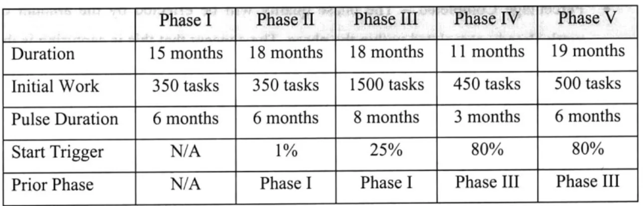
The phase duration, initial work tasks, and pulse duration as well as prior phase and start triggers for a Type 4 vehicle program are included in Table 3.

Table 3 -Phase Time and Task Constants for a Type 4 Vehicle Program

Phase I Phase II Phase IIl Phe IV Phase V Duration 15 months 18 months 18 months 11 months 19 months

Initial Work 350 tasks 350 tasks 1500 tasks 450 tasks 500 tasks

Pulse Duration 6 months 6 months 8 months 3 months 6 months

Start Trigger N/A 1% 25% 80% 80%

Prior Phase N/A Phase I Phase I Phase III Phase III

The Start Trigger and Prior Phase parameters that the start triggers and order of the phases program type.

are vehicle program type do not change depending

independent in on the vehicle

(18)

2.4 PHASE QUALITY

An important auxiliary variable that is used in the system dynamics model is the computation of the quality level within a particular phase. Basically, the quality present in a particular phase is defined as a normal quality level within the phase multiplied by a series of effects defined as follows:

" Prior Work Quality - The perceived prior work quality within a given phase will effect the quality of work performed later in the phase.

" Prior Phase Quality - The actual prior phase(s) quality will effect the quality of work accomplished within the phase.

" Schedule Pressure - The current phase quality will be effected by the amount of schedule pressure applied within the phase. This is especially true if the phase is behind schedule towards the end of the phase.

* Percentage Completed - The phase quality will be effected by the amount of work already completed within the phase. The concept that this is capturing is the fact that work done early in the phase will suffer since it is based on incomplete information that will become more complete as the phase progresses.

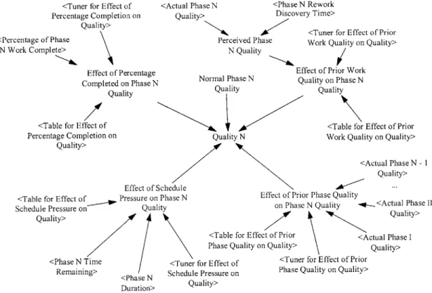
The quality variable for phases I through V, the effects on quality, and inputs to compute the multiplicative effects on quality can be seen in Figure 5.

(19)

<Tuner for Effect of <Actual Phase N <Phase N Rework Percentage Completion on Quality> Discovery Time>

Quality> _{<Tuner for Effect of Prior} <Percentage of Phase Perceived Phase Work Quality on Quality>

N Work Complete> N Quality

Effect of Percentage Effect of Prior Work Completed on Phase N Normal Phase N Quality on Phase N

Quality Quality Quality

Quality>

<Actual Phase N - I

Quality> Effect of Schedule

<Table for Effect of Pressure on Phase N Effect of Prior Phase Quality

Schedule Pressure on Quality on Phase N Quality .W- <Actual Phase 11

Quality> Quality>

<Table for Effect of Prior _{<Actual Phase I} Phase Quality on Quality> Quality> <Phase N Time <Tuner for Effect of <Tuner for Effect of Prior

Remaining> < Schedule Pressure on Phase Quality on Quality> <Phase N _Quality>

Duration>

Figure 5 -Phase N Quality

Here are the actual equations for the computation of the quality variable within a particular phase:

Effect of Percentage Completed on Phase N Quality = Tuner for Effect of Percentage Completion on Quality * Table for Effect of Percentage Completion on Quality (Percentage of Phase N Work Completed) + (1 -Tuner for Effect of Percentage Completion on Quality)

Effect of Prior Phase Quality on Phase N Quality = Tuner for Effect of Prior Phase Quality on Quality * Table for Effect of Prior Phase Quality on Quality ((Actual Phase I Quality + Actual Phase II Quality + ... + Actual Phase N-i Quality) / (N - 1)) + (1 - Tuner for Effect of Prior Phase

Quality on Quality)

(20)

Quality (Perceived Phase N Quality) + (1 - Tuner for Effect of Prior Work Quality on Quality)

Effect of Schedule Pressure on Phase N Quality = Tuner for Effect of Schedule Pressure on Quality * Table for Effect of Schedule Pressure on Quality (Phase N Time Remaining / Phase N Duration)

Perceived Phase N Quality = SMOOTHI (Actual Phase N Quality, Phase N Rework Discovery Time, 1.0)

Quality N = Normal Phase N Quality * Effect of Prior Work Quality on Phase N Quality * Effect of Prior Phase Quality on Phase N Quality * Effect of Schedule Pressure on Phase N Quality * Effect of Percentage Completed on Phase N Quality

In the above equations, the values for the lookup tables for the various effects on quality and the tuner variables that were used in the system dynamics model can be found in the Appendix. The Vensim SMOOTHI function was used to compute the delay between the actual quality level in the phase verses individual perception of quality of work within the phase. The tuner variables are used as parameters to adjust the strength or weakness of the various effects. The value for the tuner variable can range from zero (no effect) to one (full strength of the effect).

2.5 PHASE PRODUCTIVITY

An important variable in determining the work accomplished within a particular phase is the productivity level for the individuals performing work. The normal productivity variable has the units of tasks / (person * month) and is somewhat of an average assessment of personal productivity of individuals that are working on tasks within a given phase. The productivity present within a given level is defined as a normal productivity level within the phase multiplied by a series of effects defined as follows:

* Resources in Transition - Individual productivity of resources entering a vehicle program phase is half of the productivity of those resources that have been fully

(21)

incorporated into the vehicle program workforce. Basically, the effect tries to encapsulate the normal startup issues when introducing new members to an existing team and work structure.

* Schedule Pressure - Schedule pressure has a positive influence on individual productivity levels as the phase is nearing completion.

0 Strong Program Management - The application of strong program and project management within a phase will increase productivity and lessen the productivity peak that will occur due to schedule pressure at the end of the phase. The concept here is that intermediate milestones are introduced into the project plan for the phase primarily to insure that the work is spread out over the phase and does not

build up at the end of the phase.

The productivity variable for phases I through V, the effects on productivity, and the inputs to compute the multiplicative effects on productivity can be seen in Figure 6.

S I

Normal Phase N Productivity

trong Program Management Tuner for Effect of

mprovement on Productivity Phase N Productivity Schedule Pressure on Productivity

Effect of Strong Program Effect of Resource Effect of Schedule Management on Phase N Transitioning on Phase N Pressure on Phase N

Productivity Productivity Productivity

<Phase N Productive <Phase N Transition Table for Effect o

Tuner for Effect of Strong Resources> Resources> Schedule Pressure

Productivity <Phase N Duration> Productivity

Productivity Discount for _{<Phase N Time Remaining>} Transition Resources

f

on

Figure 6 -Phase N Productivity

(22)

Effect of Resources in Transition on Phase N Productivity = XIDZ (1.0 * Phase N Productive Resources + Productivity Discount for Transition Resources *

Phase N Transition Resources, Phase N Productive Resources + Phase N Transition Resources, 1.0)

Effect of Schedule Pressure on Phase N Productivity = Tuner for Effect of Schedule Pressure on Productivity * Table for Effect of Schedule Pressure on Productivity (Phase N Time Remaining / Phase N Duration) + (1

-Tuner for Effect of Schedule Pressure on Productivity)

Effect of Strong Program Management on Phase N Productivity = Tuner for Effect of Strong Program Management on Productivity * Strong Program Improvement on Productivity + (1 - Tuner for Effect of Strong Program Management on Productivity)

Productivity Discount for Transition Resources = 0.5

Phase N Productivity = Normal Phase N Productivity * Effect of Resources in Transition on Phase N Productivity * Effect of Strong Program Management on Phase N Productivity * Effect of Schedule Pressure on Phase N Productivity

In the above equations, the values for the lookup tables for the various effects on productivity and the tuner variables that were used in the system dynamics model can be found in the Appendix. The use of the Vensim XIDZ function to compute the weighted average of productivity for the productive and transition resources for the effect of resources in transition on productivity for a particular vehicle program phase and avoid an initial divide by zero condition for the model.

2.6 PHASE RESOURCES

An important aspect of a single program model, is the computation of the number of resources required within a particular phase to complete the phase work within the specified phase time duration. The mechanics of bringing staff on board within a phase,

(23)

transitioning them to fully productive employees, and releasing them back into the system when the phase work is completed is also an important aspect of the single vehicle program model. The amount of resources required to complete a particular phase on schedule is a function of the quality of work being done, the productivity of the resources in the phase, the amount of work and rework remaining in the phase, and the time remaining to complete the phase. The vehicle program managers have direct knowledge of most of these items but a few variables must be estimated due to the fact that the exact values are not known.

In order to compute the resources required to complete a particular phase, a program manager needs to estimate individual productivity. The variables used for this computation can been seen in Figure 7.

Time to Perceive Productivity

<Phase N _{Perceived Phase N} Productivity> Productivity

<Normal Phase

N Productivity>

Figure 7 -Perceived Phase N Productivity

Here is the equation for computing the perceived productivity for a particular phase:

Perceived Phase N Productivity = SMOOTHI (Phase N Productivity, Time to Perceive Productivity, Normal Phase N Productivity)

(24)

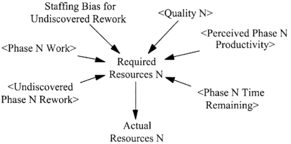
Staffing Bias for Undiscovered Rework

<Perceived Phase N <Phase N Work> Re4, e Productivity>

~-Required Resources N

<Undiscovered _{<Phase N Time}

Phase N Rework> _Remaining>

Actual Resources N

Figure 8 -Phase N Actual Resources

Here are the equations for computing the actual resources required to complete a particular phase:

Actual Resources N = Required Resources N

Required Resources N = (Phase N Work + Staffing Bias for Undiscovered Rework * Undiscovered Phase N Rework) / (Perceived Phase N Productivity * Phase N Time Remaining) / Phase N Quality

Staffing Bias for Undiscovered Rework = 1.0

The Required Resources N is a relatively simple estimate for the number of resources required in order to complete the phase on schedule. It suffers from a number of problems in reality due to the fact that the inputs into the computation (actual amount of undiscovered rework and productivity levels) are somewhat unknown to the program managers of the vehicle program. Additionally, the entering, transition, and leaving delays for placing resources into the phase (see below) are not considered in the required resource computation.

(25)

The Staffing Bias for Undiscovered Rework variable was added to the model to perform a sensitivity analysis on the estimate for the amount of resources required in order to complete a particular phase.

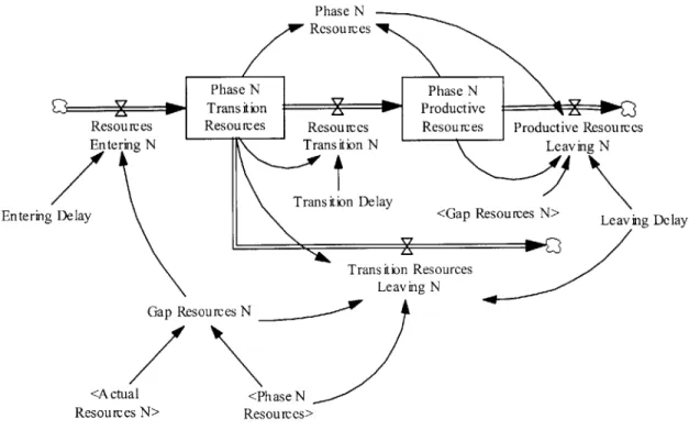
The actual resources applied within a particular phase (Phase N Resources) and the stock,

flow, and auxiliary variables that are used to compute them can bee seen in Figure 9.

Enterin

Phase N Resources

Phas4N Phase N

Transim Lion ProductiveX 0Q

Resources Resources Resources Resources Productive Resources

Entering N ~rans ition N aing N

Transition Delay

Denlay <Gap Resources N> Leaving Delay

D e l a yn D l a Transition Resources Leaving N <A ctu Resourc Gap Resources N al <Phase N es N> Resources>

Figure 9 -Phase N Resources

Here are the equations for computing the actual and required resources within a phase:

Entering Delay = 1

Gap Resources N = Phase N Resources - Actual Resources N Leaving Delay = 3

Phase N Productive Resources = INTEG (Resources Transition N - Productive Resources Leaving N, 0)

Phase N Resources = Phase N Productive Resources + Phase N Transition Resources

(26)

Phase N Transition Resources = INTEG (Resources Entering N - Resources

Transition N - Transition Resources Leaving N, 0)

Productive Resources Leaving N = MAX (0, -Gap Resources N * ZIDZ (Phase N Productive Resources, Phase N Resources) / Leaving Delay)

Resources Entering N = MAX (0, Gap Resources N / Entering Delay) Resources Transition N = Phase N Transition Resources / Transition Delay

Transition Delay = 2

Transition Resources Leaving N = MAX (0, -Gap Resources N * ZIDZ (Phase N Transition Resources, Phase N Resources) / Leaving Delay)

The amount of resources allocated to a particular phase is tracked in two stock variables, Phase N Transition Resources and Phase N Productive Resources. These variables correspond to recent vehicle program additions and the fully productive resources that have been associated with the vehicle program for quite some time.

The Entering Delay is set to a constant of one month in the system dynamics model to correspond to the time that it takes to place a resource within a vehicle program and become productive once the need has been identified. This delay is somewhat unavoidable due to the vehicle program need to collocate team members.

The Transition Delay is set to a constant of two months to correspond to the time that it takes an individual to become fully productive in the context of the vehicle program.

The Leaving Delay is set to a constant of three months in the model to correspond to a general reluctance of vehicle program team management to release people once the resource need has passed within a particular phase. There is a strong management tendency to hold onto resources to address last minute quality problems and scope

(27)

2.7 PHASE WORK ACCOMPLISHMENT

The actual work (both good and evil) accomplished within a phase depends on the amount of work available to be done and the resources applied within the phase. A first order control structure (Effect of Lack of Work on Work) was put in place on the actual work performed to ensure that the amount of work present in the Phase N Work stock would not go negative.

The actual work accomplished (Work N) within a phase and the variables that are used to compute the actual work can be seen in Figure 10.

Cumulative

<Phase N Productivity> Work N

Work N

<Phase N Work> Potential Work N

<Initial Phase N Work> <Phase N Resources>

Figure 10 -Phase N Work

Here are the actual equations for the computation of the actual work accomplished within a particular phase:

Cumulative Work N = INTEG (Work N, 0)

Potential Work N = Phase N Productivity * Phase N Resources

Work N = Potential Work N * Effect of Lack of Work on Work (Phase N Work / Initial Phase N Work)

The Cumulative Work N variable is not really required in the system dynamics model except for the generation of assessment metrics for a particular phase.

(28)

2.8 PHASE REWORK DISCOVERY TIME

The Phase N Rework Discovery Time variable determines the rate that rework is discovered and placed back into the work that needs to be accomplished for a particular phase. The rework discovery time is defined as a normal rework discovery time multiplied by a series of effects defined as follows:

" Current Phase Completion - The rework discovery time is effected by the percentage completion of the current phase.

" Future Phase Completion - The upstream rework discovery time is effected by the number of downstream phases that have completed or are nearing completion in the product development process.

As the work progresses on a particular vehicle program, the rework discovery time for each individual phase will shrink and should approach zero months near the completion of the vehicle product development process. At a conceptual level, evil work in the phase work/rework structures is detected almost as soon as it is created in the vehicle program near the completion of the last phase in the product development process.

The Phase N Rework Discovery Time variable, the effects on rework discovery time and the inputs to compute the multiplicative effects on rework discovery time can be seen in Figure 11.

(29)

<Phase N Duration>

SNormal Phase N

Rework Discovery Phase N Discovery- P Time

Pactor

<Percentage of Phase _{Phase N Rework}

N WhaseCNmRework

N Work Complete> ---- _{Phase N Effect on} _{Discovery Time}

Rework Table for Effect of Phase- Discovery Time

Completion on Rework

Discovery Time <Phase N+I Effect on

Rework Discovery Time>

Figure 11 -Phase N Rework Discovery Time

Here are the equations for the computation of rework discovery time within a particular phase:

Normal Phase N Rework Discovery Time = Phase N Duration / Phase N Discovery Factor

Phase N Effect on Rework Discovery Time = Table for Effect of Phase Completion on Rework Discovery Time (Percentage of Phase N Work Complete)

Phase N Rework Discovery Time = Normal Phase N Rework Discovery Time *

Phase N Effect on Rework Discovery Time * Phase N+1 Effect on

Rework Discovery Time * ... * Phase IV Effect on Rework Discovery

Time * Phase V Effect on Rework Discovery Time

The Normal Rework Discovery Time for a particular phase is computed based using the constants summarized in Table 4. The factors presented in table are vehicle program

(30)

Table 4 -Rework Discovery Time Constants for a Type 4 Vehicle Program

Phase I Phase Phase III Phase IV Phase V

Duration 15 Months 18 Months 18 Months 11 Months 19 Months

Discovery Factor 2 2 3 4 5

The table function for the Effect of Phase Completion on Rework Discovery Time can be found in the Appendix.

2.9 VEHICLE PROGRAM METRICS

In order to provide some meaningful characteristics or metrics for evaluating the results of a vehicle program simulation, a number of variables were added to the system dynamics model. Specifically, metrics were added to evaluate vehicle program work effort, program and phase resource utilization levels, quality levels of the phases at the scheduled completion times, and the total quality level of the vehicle program at launch.

The inputs to compute the relative vehicle program work effort (the ratio of the amount of work tasks completed to the initial work tasks for all of the vehicle program phases) can be seen in Figure 12.

(31)

<Initial Phase I Work>

<Initial Phase III Work>

Total Initial Work -4

Relative Program Work Effort <Initial Phase V Work> <Initial Phase IV Work>

<Cumulative--- _{Total Cumulative} Work-Work I> <Cumulativ Work II> e <Cumulative Work III> <Cumulative Work V> <Cumulative Work IV>

Figure 12 -Relative Program Work Effort

Here are the equations for the computation of Total Initial Work, Total Cumulative Work, and Relative Program Work Effort variables:

Relative Program Work Effort = Total Cumulative Work / Total Initial Work Total Cumulative Work = Cumulative Work I +±Cumulative Work II +

Cumulative Work III + Cumulative Work IV + Cumulative Work V

Total Initial Work = Initial Phase I Work + Initial Phase II Work + Initial Phase III Work + Initial Phase IV Work + Initial Phase V Work

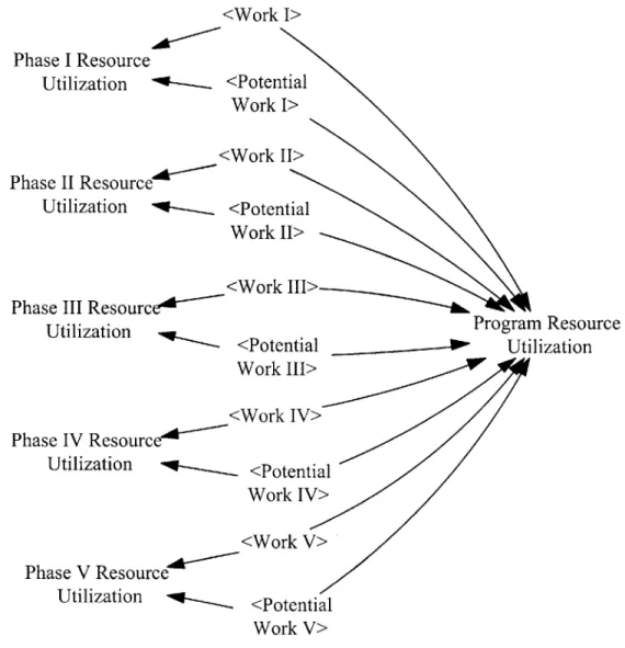
The inputs to compute the total program and program phase resource utilization variables can be seen in Figure 13.

(32)

Figure 13 -Resource Utilization

Here are the equations for computing the total vehicle program and vehicle program phase resource utilization auxiliary variables:

Phase I Resource Utilization = ZIDZ (Work I, Potential Work I) Phase II Resource Utilization = ZIDZ (Work II, Potential Work II) Phase III Resource Utilization = ZIDZ (Work III, Potential Work III) Phase IV Resource Utilization = ZIDZ (Work IV, Potential Work IV) Phase V Resource Utilization = ZIDZ (Work V, Potential Work V)

<Work I> Phase I Resource Utilization <Potential Work I> <Work II> Phase II Resource Utilization ~---.<Potential Work II>

Phase III ResourceK Work III>

Utilization - <PtnilProgram Resource

<Potential Utilization Work III> <Work IV> Phase IV Resource Utilization _<Potential Work IV> <Work V> Phase V Resource Utilization _<Potential Work V>

(33)

Program Resource Utilization = ZIDZ (Work I + Work II + Work III + Work IV

+ Work V, Potential Work I + Potential Work II + Potential Work III +

Potential Work IV + Potential Work V)

The inputs and variables to compute the final vehicle program quality and the intermediate phase quality can bee seen in Figure 14.

<Phase N Stop Time>

Final Phase N Final Phase N Quality

Quality Level

<Time> <TIME STEP>

<Actual Phase N Quality>

1OF ft-Final Progranr Final QualityQaiy

Level

<Time> <TIME STEP>

<Total Completed <Total Undiscovered Work> Rework>

Figure 14 - Final Vehicle Program and Phase Quality Values

Here are the equations for the computation of the final vehicle program quality at launch and the intermediate phase quality at phase completion times:

Final Phase N Quality = INTEG (Final Phase N Quality Level, 0)

Final Phase N Quality Level = IF THEN ELSE (Time = Phase N Stop Time, Actual Phase N Quality / TIME STEP, 0)

Final Quality Level = IF THEN ELSE (Time = Program Stop Times, (1 - ZIDZ

(Total Undiscovered Rework, Total Completed Work + Total Undiscovered Rework)) / TIME STEP, 0)

(34)

The Program Stop Times variable is equal to the Program Start Times value plus the duration of the vehicle program. In the case of a Type 4 program, the vehicle program duration is 43 months.

2.10 SUMMARY

A system dynamics model was constructed for a single vehicle program and validated

with the assistance of program engineers and managers involved with the product development process. The model contains most of the key influences on quality and productivity that occur within vehicle product development.

The only factor that could not adequately be incorporated into a system dynamics model easily was the changes introduced into the product development process as a direct result of an executive review of the program. These periodic events have a tendency to trigger rework discovery in a particular phase, classify a portion of the completed work as "scrap" within the system, or even increase the content of the vehicle program such that it is a different program type as originally specified in the cycle plan. Due to the randomness of these types of events, it was somewhat beyond the scope of this work to consider their impacts on an individual vehicle program. Any attempt to perform a calibration of a vehicle program with actual resources and work tasks would need to take these sorts of exogenous inputs into account.

The analysis and insights obtained by performing a computer simulation of the single vehicle program model will be presented in the next chapter.

(35)

3. SINGLE VEHICLE PROGRAM RESULTS AND ANALYSIS

For the process of validating the single vehicle program system dynamics model, a Type 4 vehicle program was chosen with a start date of month 7 and an end date (program launch) of month 50. The results of the computer simulation and an analysis of the output of the program model are included in the sections that follow.

3.1 WORK/REWORK STRUCTURE STOCKS AND FLOWS

The three work stocks, Work, Undiscovered Rework, and Complete Work, for the work/rework structure for a Type 4 vehicle program can be seen in Figure 15, Figure 16, and Figure 16 respectively. An interesting observation is that all of the work being done in the vehicle program after the initial Phase III work is exhausted but before Phases IV and V initiate is entirely rework related.

1,000

500

0

Vehicle Program Work (All Phases and Total)

0

Phase I Work

Phase II Work Phase III Work Phase IV Work Phase V Work Total Work 5 10 15 20 25 30 35 40 Time (month) 1 '11 3 3 -Z 45 50 55 60 65 1 1 _tasks 2 tasks 3- tI 4 4-4 4 4 4 -- - --- - - --- -- --- 4 I- C as s tasks tasks tasks

Figure 15 -Vehicle Program Work Stock

(36)

Vehicle Program Undiscovered Rework (All Phases and Total)

10 15 20 25 30 35 40 45 50 55

Time (month) Phase I Undiscovered Rework

Phase II Undiscovered Rework Phase III Undiscovered Rework Phase IV Undiscovered Rework Phase V Undiscovered Rework Total Undiscovered Rework

4,000 2,000 0 1 -4 I-1 1 tasks 2 2 2 tasks 3 3 tasks 4 4 4 tasks --- _tasks tasks

Figure 16 -Vehicle Program Undiscovered Rework Stock

Vehicle Program Complete Work (All Phases and Total)

0 5 10 15 20 25 30 35 40 45 50 55 60 65

Time (month)

Phase I Complete Work 1-Phase II Complete Work 2 Phase III Complete Work -Phase IV Complete Work

-Phase V Complete Work Total Complete Work

2 22 4 4 4 - -- - - --- -6 GG 1 tasks 2 tasks 3 3 tasks 4 4 tasks - tasks G tasks

Figure 17 -Vehicle Program Complete Work Stock

800

400

0

0 5 60 65

(37)

The four flows, Work Ramp, Good Work, Evil Work, and Rework Discovery, for the work/rework structure can be seen in Figure 18, Figure 19, Figure 20, and Figure 21 respectively. The significant drop off in the good and evil work rates in each phase can be attributed to the exhaustion of the initial work that was pulsed into the system. Since there still appears that sufficient resources are allocated within each phase to accomplish all of the tasks that reenter the work stock, the rework discovery flow appears to equal the good and evil work flows. At this point, provided that there are adequate resources, work tasks will not accumulate within the work stock. This fact suggests that the vehicle program is either over staffed or has sufficient resources to complete the rework as

quickly as it becomes discovered in the system.

Vehicle Program Work Ramp (All Phases) 200 150 100 50 0 Phase I Ramp Phase II Ramp

-Phase III Ramp Phase IV Ramp Phase V Ramp 0 5 10 15 20 25 30 Time 1 35 40 45 50 55' (month) 1 1 .3 3 3 60 65 1 tasks/month -2- tasks/month - tasks/month tasks/month tasks/month

Figure 18 -Vehicle Program Work Ramp Flow

n '-) A 1. r 1 e) -) 11

1 1

A

(38)

Vehicle Program Good Work (All Phases)

0 5 10 15 20 25 30 35 40 45 50 55

Time (month)

60

Phase I Good Work Phase II Good Work Phase III Good Work Phase IV Good Work Phase V Good Work

2 2 2 2 2 0 ' 2 4 4 - -- - -_____ _____ ___-~--- -4 1 tasks/month 2 tasks/month tasks/month 4 tasks/month n -- tasks/month

Figure 19 -Vehicle Program Good Work Flow

Vehicle Program Evil Work (All Phases) 200 150 100 50 0 0 5 10 15 20 25 30 35 40 45 Time (month) 50 55 60

Phase I Evil Work -1---Phase II Evil Work -2 Phase III Evil Work Phase IV Evil Work Phase V Evil Work

-D 4 4 4 4 14 1- tasks/month 2 tasks/month tasks/month tasks/month tasks/month

Figure 20 -Vehicle Program Evil Work Flow

200 150 100 50 0 65 65 ^ ^ C 1 11 A

(39)

Vehicle Program Rework Discovery (All Phases)

5 10 15 20 25 30 35 40

Time (month) Phase I Rework Discovery -t

Phase II Rework Discovery 2 Phase III Rework Discovery

Phase IV Rework Discovery

Phase V Rework Discovery

2 2 3 3 3 1 45 50 55 60 65 1 1 tasks/month 2 2 tasks/month 3 tasks/month 4 4 tasks/month - -tasks/month

Figure 21 -Vehicle Program Rework Discovery Flow

3.2 VEHICLE PROGRAM RESOURCES

The resources required to complete each of the vehicle program phases on time are shown in Figure 22. The apparent maximums in the resource requirements are due to the schedule deadlines imposed by program management, the delays in obtaining dedicated resources for a vehicle program, and the potentially incorrect estimates on productivity, quality, and rework for the particular phase that is being examined. The resources that have been allocated and applied to each of the vehicle program phases can be seen in Figure 23. 200 150 100 50 0 _I 0 --A--1-1/

(40)

Vehicle Program Required Resources (All Phases and Total)

F-AK ALK

5 10 15 20 25 30 35 40 45 50 55 60 65

Time (month)

Phase I Required Resources

Phase II Required Resources Phase III Required Resources Phase IV Required Resources Phase V Required Resources Total Required Resources

- -1---4 4 4 4 -4 '~ person person person person person person

Figure 22 -Vehicle Program Required Resources

Vehicle Program Applied Resources (All Phases and Total) 200

10 15 20 25 30 35 40 45

Time (month) Phase I Applied Resources

Phase II Applied Resources Phase III Applied Resources Phase IV Applied Resources Phase V Applied Resources Total Applied Resources

-9 -4 2 2 person person 3 3 person 4 4 - person - -person G 6person

Figure 23 -Vehicle Program Applied Resources

200 100 0 0 100 0 0 5 50 55 60 -1 -1 I -j 'i

(41)

The difference between the required and applied resources for a particular vehicle program phase can be seen in Figure 24. In this figure, the entering delay in obtaining resources can be seen in those cases when both of the curves are increasing and the leaving delay is present when the curves are both decreasing. These behaviors are representative of the staffing experiences of the vehicle program managers (delays in identifying and co-locating resources entering the vehicle program and a reluctance to release resources from the vehicle program teams once they are no longer required).

Phase III Required and Applied Resources

2001

I

5 10 15 20 25 30 35 40

Time (month)

45 50 55 60 65

Phase III Required Resources 1 1 1 1 1 1 1 person

Phase III Applied Resources 2 2 2 2 2 2 2 person

Figure 24 -Phase III Required and Applied Resources

3.3 VEHICLE PROGRAM PRODUCTIVITY

The vehicle program resource productivity for each of the phases can be seen in Figure

25. The effects that influence individual productivity for one of the phases, Resource

Transitioning, Schedule Pressure, and Strong Program Management, can be seen in Figure 26. The effect of resources in transition appears to be the most dominant negative

150 100 50 0 1- n ) I 0

(42)

phases. This impact can be clearly seen in the productivity levels for each of the phases when a significant number of new resources are added to the phase resource pool.

The differences between the actual productivity and the perceived productivity (used to compute the required resources for a particular phase) are shown in Figure 27. The perceived productivity for a particular vehicle program phase will be overestimated towards the start of the phase and will be underestimated at the end of the phase. If the staffing influence is examined in isolation, the management behavior will result in under staffing of resources at the beginning of the phase and over staffing towards the end of the phase. This behavior was cited by a number of vehicle program managers as a characteristic of the automotive product development process.

Vehicle Program Productivity (All Phases)

61

1

1 e)- 1 1 ' /I 1 ' -) A k- 1 ) -A 0 5 10 Phase I Productivity Phase II Productivity Phase III Productivity Phase IV Productivity Phase V Productivity 15 20 25 30 35 40 45 50 55 60 65 Time (month) 1 1 1 1 tasks/(month*person) 2 2 2 2 2 tasks/(month*person) 3 3 3 3 3 tasks/(month*person) 4 4 4 4 tasks/(month*person) - - -- _--_tasks/(month*person)

Figure 25 -Vehicle Program Productivity

4.5 3 1.5 0 -) A .

'11-

(43)

T7'--]-Phase III Productivity Effects

0 5 10 15 20 25 30 35 40 45 50 55 60 65

Time (month)

Effect of Resource Transitioning1 1 1 1 1 1 1 1 dmnl Effect of Schedule Pressurc 2 2 2 2 2 2 2 2 dmnl Effect of Strong Program Management-- 3 3 3 3 3 dmnl

Figure 26 -Phase III Productivity Effects

Phase III Current and Perceived Productivity

I

0 5 10 15 20 25 30 35 40 45 50 55 60 65

Time (month)

Current Phase III Productivity 1 1 1 1 1 tasks/(month*person)

Perceived Phase III Productivity 2 2 2 2 2 tasks/(month*person)

1.5 1.25 1 0.75 0.5 6 4.5 3 1.5 0 42 12 121

(44)

3.4 VEHICLE PROGRAM QUALITY

The vehicle program quality for each of the phases can be seen in Figure 28. The effects that influence quality for one of the phases, Percentage Completed, Prior Phases Quality, Prior Work Quality, and Schedule Pressure, can be seen in Figure 29. Generally speaking, the quality in a particular phase improves as the phase progresses due to product decisions are being made and work accomplished with more complete information from both the current phase and prior phases.

The actual and perceived quality for a particular vehicle program phase (the ratio of correctly completed work to the total amount of work that needs to be accomplished) can be seen in Figure 30.

Vehicle Program Quality (All Phases)

0.75 0.625 0.5 0.375 0.25 0 5 10 15 20 25 30 35 40 Time (month) 11 45 50 55 60 65 Phase I Quality Phase II Quality Phase III Quality Phase IV Quality Phase V Quality 1 3 3 3 3 3 3 A 4 4 4 4 f'-- --- p