Characterisation and mitigation of beam-induced backgrounds observed in the ATLAS detector during the 2011 proton-proton run

arXiv:1303.0223v3 [hep-ex] 19 Jul 2013

EUROPEAN ORGANISATION FOR NUCLEAR RESEARCH (CERN)

CERN-PH-EP-2012-313

Submitted to: JINST

Characterisation and mitigation of beam-induced backgrounds

observed in the ATLAS detector during the 2011 proton-proton

run

The ATLAS Collaboration

Abstract

This paper presents a summary of beam-induced backgrounds observed in the ATLAS detector and discusses methods to tag and remove background contaminated events in data. Trigger-rate based monitoring of beam-related backgrounds is presented. The correlations of backgrounds with machine conditions, such as residual pressure in the beam-pipe, are discussed. Results from ded-icated beam-background simulations are shown, and their qualitative agreement with data is eval-uated. Data taken during the passage of unpaired, i.e. non-colliding, proton bunches is used to obtain background-enriched data samples. These are used to identify characteristic features of beam-induced backgrounds, which then are exploited to develop dedicated background tagging tools. These tools, based on observables in the Pixel detector, the muon spectrometer and the calorimeters, are described in detail and their efficiencies are evaluated. Finally an example of an application of these techniques to a monojet analysis is given, which demonstrates the importance of such event cleaning techniques for some new physics searches.

arXiv:1303.0223v3 [hep-ex] 19 Jul 2013

Preprint typeset in JINST style - HYPER VERSION

Characterisation and mitigation of beam-induced

backgrounds observed in the ATLAS detector

during the 2011 proton-proton run

ATLAS Collaboration

E-mail: Atlas.Publications@cern.ch

ABSTRACT: This paper presents a summary of beam-induced backgrounds observed in the

AT-LAS detector and discusses methods to tag and remove background contaminated events in data. Trigger-rate based monitoring of beam-related backgrounds is presented. The correlations of back-grounds with machine conditions, such as residual pressure in the beam-pipe, are discussed. Re-sults from dedicated beam-background simulations are shown, and their qualitative agreement with data is evaluated. Data taken during the passage of unpaired, i.e. non-colliding, proton bunches is used to obtain background-enriched data samples. These are used to identify characteristic features of beam-induced backgrounds, which then are exploited to develop dedicated background tagging tools. These tools, based on observables in the Pixel detector, the muon spectrometer and the calorimeters, are described in detail and their efficiencies are evaluated. Finally an example of an application of these techniques to a monojet analysis is given, which demonstrates the importance of such event cleaning techniques for some new physics searches.

KEYWORDS: Accelerator modeling and simulations, Analysis and statistical methods, Pattern

recognition, cluster finding, calibration and fitting methods, Performance of High Energy Physics Detectors.

Contents

1. Introduction 2

2. LHC and the ATLAS interaction region 3

3. The ATLAS detector 7

4. Characteristics of BIB 9

4.1 BIB simulation methods 10

5. BIB monitoring with Level-1 trigger rates 15

5.1 BCM background rates vs residual pressure 16

5.2 BCM background rates during 2011 19

5.3 Observation of ghost charge 19

5.4 Jet trigger rates in unpaired bunches 22

6. Studies of BIB with the ATLAS Pixel detector 23

6.1 Introduction 23

6.2 Pixel cluster properties 25

6.3 Pixel cluster compatibility method 27

6.4 BIB characteristics seen in 2011 data 32

7. BIB muon rejection tools 32

7.1 General characteristics 33

7.2 BIB identification methods 36

7.2.1 Segment method 37

7.2.2 One-sided method 37

7.2.3 Two-sided method 38

7.2.4 Efficiency and mis-identification probability 38

7.3 BIB rate in 2011 40

8. Removal of non-collision background with jet observables 42

8.1 Jet cleaning 42

8.1.1 Event samples 42

8.1.2 Criteria to remove non-collision background 43

8.1.3 Evaluation of the jet quality selection efficiency 44

8.2 Monojet analysis 44

8.3 Summary of jet cleaning techniques 50

A. Alternative methods for BIB identification in the calorimeters 53

A.1 Beam background signatures in the Tile calorimeter 53

A.2 Cluster shape 54

1. Introduction

In this paper, analyses of beam induced backgrounds (BIB) seen in the ATLAS detector during the 2011 proton-proton run are presented. At every particle accelerator, including the LHC [1], particles are lost from the beam by various processes. During LHC high-luminosity running, the loss of beam intensity to proton-proton collisions at the experiments has a non-negligible impact on the beam lifetime. Beam cleaning, i.e. removing off-momentum and off-orbit particles is another important factor that reduces the beam intensity. Most of the cleaning losses are localised in special insertions far from the experiments, but a small fraction of the proton halo ends up on collimators close to the high-luminosity experiments. This distributed cleaning on one hand mitigates halo losses in the immediate vicinity of the experiments, but by intercepting some of the halo these collimators themselves constitute a source of background entering the detector areas.

Another important source of BIB is beam-gas scattering, which takes place all around the accelerator. Beam-gas events in the vicinity of the experiments inevitably lead to background in the detectors.

In ATLAS most of these backgrounds are mitigated by heavy shielding hermetically plugging the entrances of the LHC tunnel. However, in two areas of the detector, BIB can be a concern for operation and physics analyses:

• Background close to the beam-line can pass through the aperture left for the beam and cause large longitudinal clusters of energy deposition, especially in pixel detectors close to the interaction point (IP), increasing the detector occupancy and in extreme cases affecting the track reconstruction by introducing spurious clusters.

• High-energy muons are rather unaffected by the shielding material, but have the potential to leave large energy deposits via radiative energy losses in the calorimeters, where the energy

gets reconstructed as a jet. These fake jets1 need to be identified and removed in physics

analyses which rely on the measurement of missing transverse energy (E_Tmiss) and on jet

identification. This paper presents techniques capable of tagging events with fake jets due to BIB.

An increase in occupancy due to BIB, especially when associated with large local charge deposition, can increase the dead-time of front-end electronics and lead to a degradation of

data-taking efficiency. In addition the triggers, especially those depending on E_Tmiss, can suffer from rate

increases due to BIB.

1_{In this paper jet candidates originating from proton-proton collision events are called “collision jets” while jet}

This paper first presents an overview of the LHC beam structure, beam cleaning and inter-action region layout, to the extent that is necessary to understand the background formation. A concise description of the ATLAS detector, with emphasis on the sub-detectors most relevant for background studies is given. This is followed by an in-depth discussion of BIB characteristics, presenting also some generic simulation results, which illustrate the main features expected in the data. The next sections present background monitoring with trigger rates, which reveal interesting correlations with beam structure and vacuum conditions. This is followed by background observa-tions with the Pixel detector, which are compared with dedicated simulation results. The rest of the paper is devoted to fake-jet rates in the calorimeters and various jet cleaning techniques, which are effective with respect to BIB, but also other non-collisions backgrounds, like instrumental noise and cosmic muon induced showers.

2. LHC and the ATLAS interaction region

During the proton-proton run in 2011, the LHC operated at the nominal energy of 3.5 TeV for both beams. The Radio-Frequency (RF) cavities, providing the acceleration at the LHC, operate at a frequency of 400 MHz. This corresponds to buckets every 2.5 ns, of which nominally every tenth can contain a proton bunch. To reflect this sparse filling, groups of ten buckets, of which one can contain a proton bunch, are assigned the same Bunch Crossing IDentifier (BCID), of which there are 3564 in total. The nominal bunch spacing in the 2011 proton run was 50 ns, i.e. every second BCID was filled. Due to limitations of the injection chain the bunches are collected in trains, each containing up to 36 bunches. Typically four trains form one injected batch. The normal gap between trains within a batch is about 200 ns, while the gap between batches is around 900 ns. These train lengths and gaps are dictated by the injector chain and the injection process. In

addition a 3µs long gap is left, corresponding to the rise-time of the kicker magnets of the beam

abort system. The first BCID after the abort gap is by definition numbered as 1.

A general layout of the LHC, indicating the interaction regions with the experiments as well as the beam cleaning insertions, is shown in Fig. 1.

The beams are injected from the Super Proton Synchrotron (SPS) with an energy of 450 GeV in several batches and captured by the RF of the LHC. When the injection is complete the beams

are accelerated to full energy. When the maximum energy is reached the next phase is the β

-squeeze2, during which the optics at the interaction points are changed from an injection value of

β∗_{= 11 m to a lower value, i.e. smaller beam size, at the IP. Finally the beams are brought into}

collision, after which stable beams are declared and physics data-taking can commence. The phases prior to collisions, but at full energy, are relevant for background measurements because they allow the rates to be monitored in the absence of the overwhelming signal rate from the proton-proton interactions.

The number of injected bunches varied from about 200 in early 2011 to 1380 during the final phases of the 2011 proton-proton run. Typically, 95% of the bunches were colliding in ATLAS. The pattern also included empty bunches and a small fraction of non-colliding, unpaired, bunches. Nominally the empty bunches correspond to no protons passing through ATLAS, and are useful

2_{Theβ-function determines the variation of the beam envelope around the ring and depends on the focusing}

Momentum Cleaning ALICE Low ɴ (Ions) Injection RF CMS Low ɴ (protons) Dump Betatron Cleaning LHCb B-Physics Injection ATLAS Low ɴ (protons)

Figure 1. The general layout of the LHC [2]. The dispersion suppressors (DSL and DSR) are sections

between the straight section and the regular arc. In this paper they are considered to be part of the arc, for simplicity. LSS denotes the Long Straight Section – roughly 500 m long parts of the ring without net bending. All insertions (experiments, cleaning, dump, RF) are located in the middle of these sections. Beams are injected through transfer lines TI2 and TI8.

for monitoring of detector noise. The unpaired bunches are important for background monitoring in ATLAS. It should be noted that these bunches were colliding in some other LHC experiments. They were introduced by shifting some of the trains with respect to each other, such that unpaired bunches appeared in front of a train in one beam and at the end in the other. In some fill patterns some of these shifts overlapped such that interleaved bunches with only 25 ns separation were introduced.

The average intensities of bunches in normal physics operation evolved over the year from

∼ 1.0×1011_{p/bunch to∼ 1.4×10}11_{p/bunch. The beam current at the end of the year was about}

300 mA and the peak luminosity in ATLAS was 3_.5×1033cm−2s−1.

Due to the close bunch spacing, steering the beams head-on would create parasitic collisions

outside of the IP. Therefore a small crossing angle is used; in 2011 the full angle was 240µrad in

the vertical plane. In the high-luminosity interaction regions the number of collisions is maximised

mid-Figure 2. Detailed layout of the ATLAS interaction region [1]. The inner triplet consists of quadrupole

magnets Q1, Q2 and Q3. The tertiary collimator (TCT) is not shown but is located between the neutral absorber (TAN) and the D2 magnet.

September 2011.

A detailed layout of the ATLAS interaction region (IR1) is shown in Fig. 2. Inside the inner triplet and up to the neutral absorber (TAN), both beams use the same beam pipe. In the arc, beams travel in separate pipes with a horizontal separation of 194 mm. The separation and recombination of the beams happens in dipole magnets D1 and D2 with distances to the IP of 59–83 m and 153– 162 m, respectively. The D1 magnets are rather exceptional for the LHC, since they operate at room temperature in order to sustain the heat load due to debris from the interaction points. The TAS absorber, at 19 m from the IP, is a crucial element to protect the inner triplet against the heat load due to collision products from the proton-proton interactions. It is a 1.8 m long copper block with a 17 mm radius aperture for the beam. It is surrounded by massive steel shielding to reduce radiation levels in the experimental cavern [4]. The outer radius of this shielding extends far enough to cover the tunnel mouth entirely, thereby shielding ATLAS from low-energy components of BIB.

The large stored beam energy of the LHC, in combination with the heat sensitivity of the su-perconducting magnets, requires highly efficient beam cleaning. This is achieved by two separate cleaning insertions [6–8]: betatron cleaning at LHC point 7 and momentum cleaning at point 3. In these insertions a two-stage collimation takes place, as illustrated in Fig. 3. Primary collimators (TCP) intercept particles that have left the beam core. Some of these particles are scattered and re-main in the LHC acceptance, constituting the secondary halo, which hits the secondary collimators. Tungsten absorbers are used to intercept any leakage from the collimators. Although the combined

local efficiency3 of the the system is better than 99.9 % [8], some halo – called tertiary halo –

es-capes and is lost elsewhere in the machine. The inner triplets of the high-luminosity experiments represent limiting apertures where losses of tertiary halo would be most likely. In order to pro-tect the quadrupoles, dedicated tertiary collimators (TCT) were introduced at 145–148 m from the high-luminosity IP’s on the incoming beam side. The tungsten jaws of the TCT were set in 2011

to 11.8σ, while the primary and secondary collimators at point 7 intercepted the halo at 5.7σ

and 8.5σ, respectively.4 _{Typical loss rates at the primary collimators were between 10}8_–109_p/s

during the 2011 high luminosity operation. These rates are comparable to about 108proton-proton

3_{Here the local efficiency (ε}

loc) is defined such that on no element of the machine is the loss a fraction larger than

1−εlocof the total.

4_{Hereσis the transverse betatronic beam standard deviation, assuming a normalised emittance of 3.5µm. In 2011}

Figure 3. Schematic illustration of the LHC cleaning system. Primary and secondary collimators and

absorbers in the cleaning insertions remove most of the halo. Some tertiary halo escapes and is intercepted close to the experiments by the TCT [5].

events/s in both ATLAS and CMS, which indicates that the beam lifetime was influenced about equally by halo losses and proton-proton collisions. The leakage fraction reaching the TCT was

measured to be in the range 10−4–10−3[8, 9], resulting in a loss rate on the order of 105p/s on the

TCT.

The dynamic residual pressure, i.e. in the presence of a nominal beam, in the LHC beam

pipe is typically of the order of 10−9 mbar N2-equivalent5 in the cold regions. In warm sections

cryo-pumping, i.e. condensation on the cold pipe walls, is not available and pressures would be higher. Therefore most room-temperature sections of the vacuum chambers are coated with a spe-cial Non-Evaporative Getter (NEG) layer [10], which maintains a good vacuum and significantly reduces secondary electron yield. There are, however, some uncoated warm sections in the vicinity of the experiments. In 2010 and 2011 electron-cloud formation [11, 12] in these regions led to an increase of the residual pressure when the bunch spacing was decreased. As an emergency mea-sure, in late 2010, small solenoids were placed around sections where electron-cloud formation was observed (58 m from the IP). These solenoids curled up the low-energy electrons within the vacuum, suppressing the multiplication and thereby preventing electron-cloud build-up. During a campaign of dedicated "scrubbing" runs with high-intensity injection-energy beams, the surfaces were conditioned and the vacuum improved. After this scrubbing, typical residual pressures in the

5_{The most abundant gases are H}

2, CO, CO2and CH4. For simplicity a common practice is to describe these with an

warm sections remained below 10−8mbar N2-equivalent in IR1 and were practically negligible in

NEG coated sections – as predicted by early simulations [13].

3. The ATLAS detector

The ATLAS detector [14] at the LHC covers nearly the entire solid angle around the interaction

point with calorimeters extending up to a pseudorapidity_|η_{| = 4.9. Here}η_{= −ln(tan(}θ/2)), with

θ being the polar angle with respect to the nominal LHC beam-line.

In the right-handed ATLAS coordinate system, with its origin at the nominal IP, the azimuthal

angleφ is measured with respect to the x-axis, which points towards the centre of the LHC ring.

Side A of ATLAS is defined as the side of the incoming clockwise LHC beam-1, while the side of the incoming beam-2 is labelled C. The z-axis in the ATLAS coordinate system points from C to A, i.e. along the beam-2 direction.

ATLAS consists of an inner tracking detector (ID) in the_|η_{| < 2.5 region inside a 2 T}

super-conducting solenoid, which is surrounded by electromagnetic and hadronic calorimeters, and an external muon spectrometer with three large superconducting toroid magnets. Each of these

mag-nets consists of eight coils arranged radially and symmetrically around the beam axis. The high-η

edge of the endcap toroids is at a radius of 0.83 m and they extend to a radius of 5.4 m. The barrel toroid is at a radial distance beyond 4.3 m and is thus not relevant for studies in this paper.

The ID is responsible for the high-resolution measurement of vertex positions and momenta of charged particles. It comprises a Pixel detector, a silicon tracker (SCT) and a Transition Radi-ation Tracker (TRT). The Pixel detector consists of three barrel layers at mean radii of 50.5 mm, 88.5 mm and 122.5 mm each with a half-length of 400.5 mm. The coverage in the forward region is provided by three Pixel disks per side at z-distances of 495 mm, 580 mm and 650 mm from the

IP and covering a radial range between 88.8–149.6 mm. The Pixel sensors are 250µm thick and

have a nominal pixel size of rφ_{× z = 50 × 400}µm2. At the edge of the front-end chip there are

linked pairs of “ganged” pixels which share a read-out channel. These ganged pixels are typically excluded in the analyses presented in this paper.

The ATLAS solenoid is surrounded by a high-granularity liquid-argon (LAr) electromagnetic calorimeter with lead as absorber material. The LAr barrel covers the radial range between 1.5 m

and 2 m and has a half-length of 3.2 m. The hadronic calorimetry in the region_|η_{| < 1.7 is provided}

by a scintillator-tile calorimeter (TileCal), while hadronic endcap calorimeters (HEC) based on

LAr technology are used in the region 1_{.5 < |}η_{| < 3.2. The absorber materials are iron and copper,}

respectively. The barrel TileCal extends from r= 2.3 m to r = 4.3 m and has a total length of

8.4 m. The endcap calorimeters cover up to|η| = 3.2, beyond which the coverage is extended by

the Forward Calorimeter (FCAL) up to_|η_{| = 4.9. The high-}η edge of the FCAL is at a radius

of_{∼ 70 mm and the absorber materials are copper (electromagnetic part) and tungsten (hadronic}

part). Thus the FCAL is likely to provide some shielding from BIB for the ID. All calorimeters provide nanosecond timing resolution.

The muon spectrometer surrounds the calorimeters and is composed of a Monitored Drift Tube

(MDT) system, covering the region of_|η_{| < 2.7 except for the innermost endcap layer where the}

coverage is limited to_|η_{| < 2. In the |}η_{| > 2 region of the innermost layer, Cathode-Strip Chambers}

The timing resolution of the muon system is 2.5 ns for the MDT and 7 ns for the CSC. The

first-level muon trigger is provided by Resistive Plate Chambers (RPC) up to_|η_{| = 1.05 and Thin Gap}

Chambers (TGC) for 1_{.05 < |}η_{| < 2.4.}

Another ATLAS sub-detector extensively used in beam-related studies is the Beam Condi-tions Monitor (BCM) [15]. Its primary purpose is to monitor beam condiCondi-tions and detect anoma-lous beam-losses which could result in detector damage. Aside from this protective function it is also used to monitor luminosity and BIB levels. It consists of two detector stations (forward and backward) with four modules each. A module consists of two polycrystalline chemical-vapour-deposition (pCVD) diamond sensors, glued together back-to-back and read out in parallel. The

modules are positioned at z_{= ±184 cm, corresponding to z/c = 6.13 ns distance to the interaction}

point. The modules are at a radius of 55 mm, i.e. at an _|η_{| of about 4.2 and arranged as a cross}

– two modules on the vertical axis and two on the horizontal. The active area of each sensor is

8_{× 8mm}2. They provide a time resolution in the sub-ns range, and are thus well suited to identify

BIB by timing measurements.

In addition to these main detectors, ATLAS has dedicated detectors for forward physics and luminosity measurement (ALFA, LUCID, ZDC), of which only LUCID was operated throughout the 2011 proton run. Despite the fact that LUCID is very close to the beam-line, it is not partic-ularly useful for background studies, mainly because collision activity entirely masks the small background signals.

An ATLAS data-taking session (run) ideally covers an entire stable beam period, which can last several hours. During this time beam intensities and luminosity, and thereby the event rate, change significantly. To optimise the data-taking efficiency, the trigger rates are adjusted several times during a run by changing the trigger prescales. To cope with these changes and those in detector conditions, a run is subdivided into luminosity blocks (LB). The typical length of a LB in the 2011 proton-proton run was 60 seconds. The definition contains the intrinsic assumption that during a LB the luminosity changes by a negligible amount. Changes to trigger prescales and any other settings affecting the data-taking are always aligned with LB boundaries.

In order to assure good quality of the analysed data, lists of runs and LBs with good beam conditions and detector performance are used. Furthermore, there are quality criteria for various reconstructed physics objects in the events that help to distinguish between particle response and noise. In the context of this paper, it is important to mention the quality criteria related to jets

re-constructed in the calorimeters. The jet candidates used here are rere-constructed using the anti-kt jet

clustering algorithm [16] with a radius parameter R= 0.4, and topologically connected clusters of

calorimeter cells [17] are used as input objects. Energy deposits arising from particles showering in the calorimeters produce a characteristic pulse in the read-out of the calorimeter cells that can be used to distinguish ionisation signals from noise. The measured pulse is compared with the

expec-tation from simulation of the electronics response, and the quadratic difference Qcellbetween the

actual and expected pulse shape is used to discriminate noise from real energy deposits.6 Several

jet-level quantities can be derived from the following cell-level variables:

6_Q

cellis computed online using the measured samples of the pulse shape in time as

Q_cell= N

∑

• fHEC: Fraction of the jet energy in the HEC calorimeter.

• hQi: The average jet quality is defined as the energy-squared weighted average of the pulse

quality of the calorimeter cells (Qcell) in the jet. This quantity is normalised such that 0<

hQi < 1.

• fLAr

Q : Fraction of the energy in LAr calorimeter cells with poor signal shape quality (Qcell>

4000).

• fHEC

Q : Fraction of the energy in the HEC calorimeter cells with poor signal shape quality

(Qcell> 4000).

• Eneg: Energy of the jet originating from cells with negative energy that can arise from

elec-tronic noise or early out-of-time pile-up7.

4. Characteristics of BIB

At the LHC, BIB in the experimental regions are due mainly to three different processes [19–21]: • Tertiary halo: protons that escape the cleaning insertions and are lost on limiting apertures,

typically the TCT situated at_{|z| ≈ 150m from the IP.}

• Elastic beam-gas: elastic beam-gas scattering, as well as single diffractive scattering, can result in small-angle deflections of the protons. These can be lost on the next limiting aperture before reaching the cleaning insertions. These add to the loss rate on the TCTs.

• Inelastic beam-gas: inelastic beam-gas scattering results in showers of secondary particles. Most of these have only fairly local effects, but high-energy muons produced in such events can travel large distances and reach the detectors even from the LHC arcs.

By design, the TCT is the main source of BIB resulting from tertiary halo losses. Since it is in the straight section with only the D1 dipole and inner triplet separating it from the IP, it is expected that the secondary particles produced in the TCT arrive at rather small radii at the experiment. The losses on the TCT depend on the leakage from the primary collimators, but also on other bottlenecks in the LHC ring. Since the betatron cleaning is at LHC point 7, halo of the clockwise beam-1 has to pass two LHC octants to reach ATLAS, while beam-2 halo has six octants to cover,

with the other low-β experiment, CMS, on the way. Due to this asymmetry, BIB due to losses on

the TCT cannot be assumed to be symmetric for both beams.

There is no well-defined distinction between halo and elastic beam-gas scattering because scattering at very small angles feeds the halo, the formation of which is a multi-turn process as protons slowly drift out of the beam core until they hit the primary collimators in the cleaning insertions at IP3 and IP7. Some scattering events, however, lead to enough deflection that the where A is the measured amplitude of the signal [18], sjis the amplitude of each sample j, and gphysj is the normalised

predicted ionisation shape.

7_{Out-of-time pile-up refers to proton-proton collisions occurring in BCIDs before or after the triggered collision}

protons are lost on other limiting apertures before they reach the cleaning insertions. The most likely elements at which those protons can be lost close to the experiments are the TCTs. The rate of such losses is in addition to the regular tertiary halo. This component is not yet included in the simulations, but earlier studies based on 7 TeV beam energy suggest that it is of similar magnitude as the tertiary halo [20]. The same 7 TeV simulations also indicate that the particle distributions at the experiment are very similar to those due to tertiary halo losses.

The inelastic beam-gas rate is a linear function of the beam intensity and of the residual pres-sure in the vacuum chamber. The composition of the residual gas depends on the surface charac-teristics of the vacuum chamber and is different in warm and cryogenic sections and in those with NEG coating. Although several pressure gauges are present around the LHC, detailed pressure maps can be obtained only from simulation similar to those described in [22]. The gauges can then be used to cross-check the simulation results at selected points. The maps allow the expected rate of beam-gas events to be determined. Such an interaction distribution, calculated for the conditions of LHC fill 2028, is shown in Fig. 4. The cryogenic regions, e.g. inner triplet (23–59m), the

mag-nets D2 & Q4, Q5 and Q6 at∼ 170 m, ∼ 200 m and ∼ 220 m, respectively, and the arc (>269 m),

are clearly visible as regions with a higher rate, while the NEG coating of warm sections efficiently suppresses beam-gas interactions. The TCT, being a warm element without NEG coating,

pro-duces a prominent spike at_{∼ 150 m. In the simulations it is assumed that the rate and distribution}

of beam-gas events are the same for both beams.

4.1 BIB simulation methods

The simulation of BIB follows the methods first outlined in [19], in particular the concept of a two-phase approach with the machine and experiment simulations being separate steps. In the first phase the various sources of BIB are simulated for the LHC geometry [9, 21]. These simulations

produce a file of particles crossing an interface plane at z= 22.6 m from the IP. From this plane

onwards, dedicated detector simulations are used to propagate the particles through the experimen-tal area and the detector. Contrary to earlier studies [19, 20, 23], more powerful CPUs available

today allow the machine simulations to be performed without biasing.8 This has the advantage of

preserving all correlations within a single event and thus allows event-by-event studies of detector response. The beam halo formation and cleaning are simulated with SixTrack [24], which com-bines optical tracking and Monte Carlo simulation of particle interactions in the collimators. The inelastic interactions, either in the TCT based on the impact coordinates from SixTrack, or with

residual gas, are simulated with FLUKA[25]. The further transport of secondary particles up to the

interface plane is also done with FLUKA.

High-energy muons are the most likely particles to cause fake jet signals in the calorime-ters. At sufficiently large muon energies, typically above 100 GeV, radiative energy losses start to dominate and these can result in local depositions of a significant fraction of the muon energy via electromagnetic and, rarely, hadronic cascades [26].

8_{There are several biasing techniques available in Monte Carlo simulations. All of these aim at increasing statistics}

in some regions of phase space at the cost of others by modifying the physical probabilities and compensating this by assigning non-unity statistical weights to the particles. As an example the life-time of charged pions can be decreased in order to increase muon statistics. The statistical weight of each produced muon is then smaller than one so that on average the sum of muon weights corresponds to the true physical production rate.

Distance from IP [m]

0

50 100 150 200 250 300 350

Beam-gas interaction rate [Hz/m/proton]

10

10

10

Interface plane & 22m VAC-gauge 58m VAC-gauge TCT(c) Arc LSS Inner triplet

LHC Simulation

Figure 4. Inelastic beam-gas interaction rates per proton, calculated for beam-1 in LHC fill 2028. The

machine elements of main interest are indicated. The pressure in the arc is assumed to be constant from 270 m onwards. The letters, a-e, identify the different sections, for which rates are given separately in other plots.

The TCTs are designed to intercept the tertiary halo. Thus they represent intense – viewed from the IP, almost point-like – sources of high-energy secondary particles. The TCTs are in the straight section and the high-energy particles have a strong Lorentz boost along z. Although they have to traverse the D1 magnet and the focusing quadrupoles before reaching the interface plane, most of the muons above 100 GeV remain at radii below 2 m.

The muons from inelastic beam-gas events, however, can originate either from the straight section or from the arc. In the latter case they emerge tangentially to the ring or pass through several bending dipoles, depending on energy and charge. Both effects cause these muons to be spread out in the horizontal plane so that their radial distribution at the experiment shows long tails, especially towards the outside of the ring.

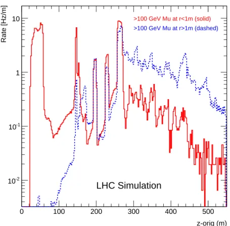
In the following, some simulation results are shown, based on the distribution of muons with momentum greater than 100 GeV at the interface plane. The reason to restrict the discussion to muons is twofold:

z-orig (m) 0 100 200 300 400 500 Rate [Hz/m] -2 10 -1 10 1 10 >100 GeV Mu at r<1m (solid) >100 GeV Mu at r>1m (dashed)

LHC Simulation

Figure 5. Simulated distribution of the z-coordinates of inelastic beam-gas events from which a muon with

more than 100 GeV has reached the interface plane at 22.6 m. The two curves correspond to muons at radii below and above 1 m at the interface plane.

material. All hadrons and EM-particles, except those within the 17 mm TAS aperture or at radii outside the shielding, undergo scattering and result in a widely spread shower of secondary particles. Therefore the distributions of these particles at the interface plane do not directly reflect what can be seen in the detector data.

2. High-energy muons are very penetrating and rather unaffected by material, but they are also the cause of beam-related calorimeter background. Therefore the distribution of high-energy muons is expected to reflect the fake jet distribution seen in data. The muon component is less significant for the ID, but its distribution can still reveal interesting effects.

Figure 5 shows the simulated z-distribution of inelastic beam-gas events resulting in a high-energy muon at the interface plane. In order to reach larger radii the muons have to originate from

more distant events. Since the barrel calorimeters9, which detect the possible fake jets, cover radii

above 1 m, the fake jet rate is not expected to be sensitive to close-by beam-gas interactions and

9_{Fake jets can be produced also in the endcap and forward calorimeters, but due to higher rapidity are less likely to}

R [cm]

0

200

400

600

800

1000 1200

]

Rate [Hz/cm

10

10

10

10

10

10

10

10

1

10

a) >100 GeV beam-gas Muons from z=22.6-59m b) >100 GeV beam-gas Muons from z=59-153m

c) >100 GeV Muons from Beam-2 TCT

d) >100 GeV beam-gas Muons from z=153-269m

e) >100 GeV beam-gas Muons from z>269m

e)

d)

b) c)

a)

LHC Simulation

Figure 6. Simulated radial distribution at the interface plane of muons from inelastic beam-gas collisions

and from the beam-2 TCT. The four solid curves correspond to muons originating from beam-gas events in different regions of the LSS and the adjacent LHC arc. The dashed curve shows the distribution of muons

from the beam-2 TCT, normalised to 105p/s lost on the TCT. The letters refer to the regions indicated in

Fig. 4.

therefore not to the pressure in the inner triplet. This is discussed later in the context of correlations

between background rates and pressures seen by the vacuum gauges at_{|z| = 22 m and |z| = 58 m.}

Figure 6 shows the simulated radial distributions of high-energy muons from inelastic beam-gas events taking place at various distances from the IP. Figure 4 suggests that the regions with highest interaction rate are the inner triplet, the TCT region, the cold sections in the LSS beyond the TCT, and the arc. In NEG-coated warm regions the expected beam-gas rate is negligible, which allows the interesting sections to be grouped into four wide regions, as indicated at the bottom of Fig. 4. It is evident from Fig. 6 that at very small radii beam-gas interactions in the inner triplet dominate, but these do not give any contributions at radii beyond 1 m. The radial range between 1–4 m, covered by the calorimeters, gets contributions from all three distant regions, but

the correlation between distance and radius is very strong and in the TileCal (r= 2–4 m) muons

from the arc dominate by a large factor. Beyond a radius of 4 m only the arc contributes to the high-energy muon rate.

[rad] φ -3 -2 -1 0 1 2 3 Rate [Hz] -4 10 -3 10 -2 10 -1 10 1 10

a) >100 GeV Muons from z=22.6-59 m

b) >100 GeV Muons from z=59-153 m d) >100 GeV Muons from z=153-269 m

e) >100 GeV Muons from z>269 m

LHC Simulation R<100 cm (b) (e) (d) (a) [rad] φ -3 -2 -1 0 1 2 3 Rate [Hz] -4 10 -3 10 -2 10 -1 10 1 10 R=100-200 cm LHC Simulation (d) (e) _(b) [rad] φ -3 -2 -1 0 1 2 3 Rate [Hz] -4 10 -3 10 -2 10 -1 10 1 10 R=200-400 cm LHC Simulation (d) (e) [rad] φ -3 -2 -1 0 1 2 3 Rate [Hz] -4 10 -3 10 -2 10 -1 10 1 10 R>400 cm LHC Simulation (e)

Figure 7. Simulated azimuthal distribution of beam-gas muons at the interface plane in four different radial

ranges. The regions of origin considered are the same as in Fig. 6. The values have not been normalised to unit area, but represent the rate over the entire surface - which is different in each plot. The letters refer to the regions indicated in Fig. 4. The contribution from nearby regions drops quickly with radius. Histograms with negligible contribution have been suppressed.

tions in the TCT, which represents a practically point-like source situated at slightly less than 150 m from the IP. It can be seen that the radial distribution is quite consistent with that of beam-gas

colli-sions in the z= 59–153 m region. The TCT losses lead to a fairly broad maximum below r = 1 m,

followed by a rapid drop, such that there are very few high-energy muons from the TCT at r> 3 m.

The absolute level, normalised to the average loss rate of 105p/s on the TCT, is comparable to that

expected from beam-gas collisions.

Figure 7 shows the simulated φ-distribution of the high-energy muons for different radial

ranges and regions of origin of the muons. At radii below 1 m the muons from the inner triplet show a structure with four spikes, created by the quadrupole fields of the focusing magnets. Muons from more distant locations are deflected in the horizontal plane by the separation and recom-bination dipoles creating a structure with two prominent spikes. The figure shows both charges

together, but actually D1 separates, according to charge, the muons originating from within 59-153 m. Since D2 has the same bending power but in the opposite direction, muons from farther

away are again mixed. The same two-spiked structure is also seen at larger radii. Beyond r= 2 m

a slight up-down asymmetry is observed, which can be attributed to a non-symmetric position of the beam-line with respect to the tunnel floor and ceiling – depending on the region, the beam-line is about 1 m above the floor and about 2 m below the ceiling. This causes a different free drift for upward- and downward-going pions and kaons to decay into muons before interacting in ma-terial. Since the floor is closer than the roof, fewer high-energy muons are expected in the lower hemisphere. A similar up-down asymmetry was already observed in calorimetric energy depo-sition when 450 GeV low-intensity proton bunches were dumped on the TCT during LHC beam commissioning [27], although in this case high-energy muons probably were a small contribution to the total calorimeter energy. Finally, at radii beyond 4 m, only muons from the arc contribute.

The peak at_|φ_{| =}πis clearly dominant, and is due to the muons being emitted tangentially to the

outside of the ring.

5. BIB monitoring with Level-1 trigger rates

The system that provides the Level-1 (L1) trigger decision, the ATLAS Central Trigger Processor (CTP) [28], organises the BCIDs into Bunch Groups (BG) to account for the very different char-acteristics, trigger rates, and use-cases of colliding, unpaired, and empty bunches. The BGs are adapted to the pattern of each LHC fill and their purpose is to group together BCIDs with similar characteristics as far as trigger rates are concerned. In particular, the same trigger item can have different prescales in different BGs.

The BGs of interest for background studies are:

• BGRP0, all BCIDs, except a few at the end of the abort gap • Paired, a bunch in both LHC beams in the same BCID

• Unpaired isolated (UnpairedIso), a bunch in only one LHC beam with no bunch in the other

beam within_{± 3 BCIDs.}

• Unpaired non-isolated (UnpairedNonIso), a bunch in only one LHC beam with a nearby bunch (within three BCIDs) in the other beam.

• Empty, a BCID containing no bunch and separated from any bunch by at least five BCIDs. The L1 trigger items which were primarily used for background monitoring in the 2011 proton run are summarised in Table 1 and explained in the following.

The L1_BCM_AC_CA trigger is defined to select particles travelling parallel to the beam, from side A to side C or vice-versa. It requires a background-like coincidence of two hits, defined

as one (early) hit in a time window_{−6.25± 2.73 ns before the nominal collision time and the other}

(in-time) hit in a time window_{+6.25 ± 2.73 ns after the nominal collision time.}

Table 1 lists two types of BCM background-like triggers – one in BGRP0, and the other in the UnpairedIso BG. The motivation to move from L1_BCM_AC_CA_BGRP0, used in 2010 [29],

Trigger item Description Usage in background studies

L1_BCM_AC_CA_BGRP0 BCM background-like coincidence BIB level monitoring

L1_BCM_AC_CA_UnpairedIso BCM background-like coincidence BIB level monitoring

L1_BCM_Wide_UnpairedIso BCM collision-like coincidence Ghost collisions

L1_BCM_Wide_UnpairedNonIso BCM collision-like coincidence Ghost collisions

L1_J10_UnpairedIso Jet with pT> 10 GeV at L1 Fake jets & ghost collisions

L1_J10_UnpairedNonIso Jet with pT> 10 GeV at L1 Fake jets & ghost collisions

Table 1. ATLAS trigger items used during the 2011 proton runs for background studies and monitoring.

to unpaired bunches was that a study of 2010 data revealed a significant luminosity-related con-tamination due to accidental background-like coincidences in the trigger on all bunches (BGRP0). Although the time window of the trigger is narrow enough to discriminate collision products from the actually passing bunch, each proton-proton event is followed by afterglow [30], i.e. delayed tails of the particle cascades produced in the detector material. The afterglow in the BCM is

exponentially falling and the tail extends to _{∼ 10}µs after the collision. With 50 ns bunch

spac-ing this afterglow piles up and becomes intense enough to have a non-negligible probability for causing an upstream hit in a later BCID that is in background-like coincidence with a true back-ground hit in the downstream detector arm. In the rest of this paper, unless otherwise stated, the L1_BCM_AC_CA_UnpairedIso rate before prescaling is referred to as BCM background rate.

A small fraction of the protons injected into the LHC escape their nominal bunches. If this happens in the injectors, the bunches usually end up in neighbouring RF buckets. If the bunches are within the same 25 ns BCID as the main bunch, they are referred to as satellites. If de- and re-bunching happens during RF capture in the LHC, the protons spread over a wide range of buckets and if they fall outside filled BCIDs, they are referred to as ghost charge.

The L1_BCM_Wide triggers require a collision-like coincidence, i.e. in-time hits on both sides of the IP. The time window to accept hits extends from 0.39 ns to 8.19 ns after the nominal collision time.

The L1_J10 triggers fire on an energy deposition above 10 GeV, at approximately

electromag-netic scale, in the transverse plane in an η–φ region with a width of about 0_{.8 × 0.8 anywhere}

within_|η_{| < 3.0 and, with reduced efficiency, up to}η_{| = 3.2. Like the L1_BCM_Wide triggers,}

the two L1_J10 triggers given in Table 1 are active in UnpairedIso or UnpairedNonIso bunches, which makes them suitable for studies of ghost collisions rates in these two categories of unpaired bunches.

The original motivation for introducing the UnpairedIso BG was to stay clear of this ghost charge, while the UnpairedNonIso BG was intended to be used to estimate the amount of this

component. However, as will be shown, an isolation by _{±3 BCID is not always sufficient, and}

some of the UnpairedIso bunches still have signs of collision activity. Therefore Table 1 lists the UnpairedIso BG as suitable for ghost charge studies.

5.1 BCM background rates vs residual pressure

In order to understand the origin of the background seen by the BCM, the evolution of the rates and residual pressure in various parts of the beam pipe at the beginning of an LHC fill are studied. The vacuum gauges providing data for this study are located at 58 m, 22 m and 18 m from the IP.

Time [UTC]

protons]

BCM bkgd Rate [Hz/10

mbar]

Residual Pressure [10

p]

B

e

a

m

E

n

e

rg

y

[

T

e

V

]

&

I

n

te

n

s

it

y

[

1

0

10

10

10

1

10

10

10

Inject Ramp Adjust Stable Beams

ATLAS

Pressure at z=22m (Dashed) Pressure at z=58m (Solid) Beam Intensity (Dashed) Beam Energy (Solid)

BCM bkgd Rate in UnpairedIso

LHC Fill 2210, Oct 13, 2011

Figure 8. Pressures, beam parameters and BCM background rates during the start of a typical LHC fill.

The pressures from these are referred to as P58, P22 and P18, respectively. Figure 8 shows a char-acteristic evolution of pressures and BCM background rate when the beams are injected, ramped and brought into collision. P58 starts to increase as soon as beam is injected into the LHC. The pressure, however, does not reflect itself in the background seen by the BCM. Only when the beams are ramped from 450 GeV to 3.5 TeV, does P22 increase, presumably due to increased synchrotron radiation from the inner triplet. The observed BCM background increase is disproportionate to the pressure increase. This is explained by the increasing beam energy, which causes the produced secondary particles, besides being more numerous, to have higher probability for inducing pene-trating showers in the TAS, which is between the 22 m point and the BCM. The pressure of the third gauge, located at 18 m in a NEG-coated section of the vacuum pipe, is not shown in Fig. 8. The NEG-coating reduces the pressure by almost two orders of magnitude, such that the residual

gas within_{± 19 m does not contribute significantly to the background rate. According to Fig. 4,}

the pressure measured by the 22 m gauge is constant through the entire inner triplet10. This and

the correlation with P22 suggest that the background seen by the BCM is due mostly to beam-gas events in the inner triplet region.

10_{The pressure simulation is based, among other aspects, on the distribution and intensity of synchrotron radiation,}

Pressure at 22m [mbar]

10

10

10

protons]

BCM Background Rate [Hz/10

10

1

10

Figure 9. Correlation between P22 and BCM background rate. Each dot represents one LB.

This conclusion is further supported by Fig. 9 where the BCM background rate versus P22 is shown. In the plot each point represents one LB, i.e. about 60 seconds of data-taking. Since beam intensities decay during a fill, the pressures and background rate also decrease so that individual LHC fills are seen in the plot as continuous lines of dots. A clear, although not perfect, correlation can be observed. There are a few outliers with low pressure and relatively high rate. All of these are associated with fills where P58 was abnormally high.

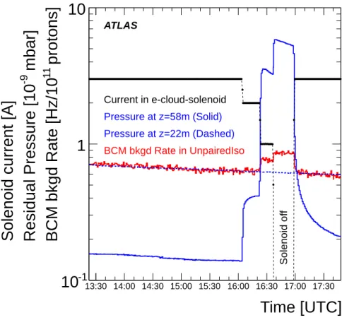
The relative influence of P22 and P58 on the BCM background was studied in a special test, where the small solenoids around the beam pipe at 58 m, intended to suppress electron-cloud for-mation, were gradually turned off and back on again. Figure 10 shows the results of this study. The solenoids were turned off in three steps and due to the onset of electron-cloud formation the pressure at 58 m increased by a factor of about 50. At the same time the pressure at 22 m showed only the gradual decrease due to intensity lifetime. With the solenoids turned off, P58 was about nine times larger than P22. At the same time the BCM background rate increased by only 30%, while it showed perfect proportionality to P22 when the solenoids were on and P58 suppressed. This allows quantifying the relative effect of P58 on the BCM background to be about 3-4% of that of P22. If these 3-4% were taken into account in Fig. 9, the outliers described above would be almost entirely brought into the main distribution.

Time [UTC]

protons]

BCM bkgd Rate [Hz/10

mbar]

Residual Pressure [10

Solenoid current [A]

-1

10

1

10

Figure 10. P58, P22 and background seen at the BCM during the “solenoid test” in LHC fill 1803. The

dashed line is not a fit, but the actual P22 value, which just happens to agree numerically with the BCM rate on this scale.

of beam-gas rate produced close to the experiment, while it has low efficiency to monitor beam losses far away from the detector.

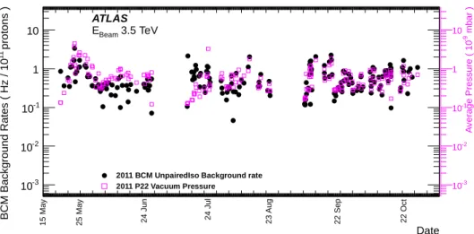
5.2 BCM background rates during 2011

Figure 11 shows the BCM background rate for the 2011 proton runs together with the P22 average residual pressure. These rates are based on the L1_BCM_AC_CA_UnpairedIso trigger rates, which became available after the May technical stop of the LHC. During the period covered by the plot, the number of unpaired bunches and their location in the fill pattern changed considerably. No obvious correlation between the scatter of the data and these changes could be identified. No particular time structure or long-term trend can be observed in the 2011 data. The average value of the intensity-normalised rate remains just below 1 Hz throughout the year.

Except for a few outliers, due to abnormally high P58, the BCM background rate correlates well with the average P22 residual pressure, in agreement with Fig. 9 and the discussion in Sect. 5.1.

5.3 Observation of ghost charge

background-Date 15 May 25 May 24 Jun 24 Jul 23

A u g 22 Sep 22 Oct protons ) 1 1 BCM Background Rates ( Hz / 10 -3 10 -2 10 -1 10 1 10

2011 BCM UnpairedIso Background rate 2011 P22 Vacuum Pressure ATLAS 3.5 TeV Beam E mbar ) -9 A v e ra g e P re s s u re ( 1 0 -3 10 -2 10 -1 10 1 10

Figure 11. BCM background rate normalised to 1011 protons for the 2011 proton-proton running period

starting from mid-May. The rate is shown together with the P22 average residual pressure.

like trigger can be used to select beam-gas events created by ghost charge. Since, for a given pressure, the beam-gas event rate is a function of bunch intensity only, this trigger yields directly the relative intensity of the ghost charge with respect to a nominal bunch, in principle. The rate, however, is small and almost entirely absorbed in backgrounds, mainly the accidental afterglow coincidences discussed at the beginning of this section. Another problem is that due to the width of the background trigger time window, only the charge in two or three RF buckets is seen, depending on how accurately the window is centred around the nominal collision time.

A more sensitive method is to look at the collisions of a ghost bunch with nominal bunches. Provided the emittance of the ghost bunches is the same as that of nominal ones, the luminosity of these collisions, relative to normal per-bunch luminosity gives directly the fraction of ghost charge in the bucket with respect to a nominal bunch. The collisions probe the ghost charge only in the nominal RF bucket, which is the only one colliding with the unpaired bunch. The charge in the other nine RF buckets of the BCID is not seen. Data from the Longitudinal Density Monitors of the LHC indicate that the ghost charge is quite uniformly distributed in all RF buckets of a non-colliding BCID [31, 32].

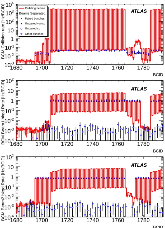
Figure 12 shows a summary of BCM collision-like and background-like trigger rates for a particularly interesting BCID range of a bunch pattern with 1317 colliding bunches. For this plot, several ATLAS runs with the same bunch-pattern and comparable initial beam intensities have been averaged. The first train of a batch is shown with part of the second train. The symbols show the trigger rates with both beams at 3.5 TeV but before they are brought into collision, while the

histograms show the rates for the first_{∼15 minutes of stable beam collisions. This restriction to the}

start of collisions is necessary since the rates are not normalised by intensity, and a longer period would have biased the histograms due to intensity decay. The groups of six unpaired bunches each in front of the beam-2 trains (around BCID 1700 and 1780, respectively) and after the beam-1 train (around BCID 1770) can be clearly seen. These show the same background trigger rate before and during collisions. As soon as the beams collide, the collision rate in paired BCIDs rises, but the background rate also increases by about an order of magnitude. As explained before, this increase

BCID

1680

1700

1720

1740

1760

1780

BCM Collision rate [Hz/BCID]

-3

10

10

10

1

10

10

10

10

Beams Separated: ATLAS

BCID

1680

1700

1720

1740

1760

1780

BCM Beam1 bkgd Rate [Hz/BCID] -4

10

10

10

10

1

10

10

1680

1700

1720

1740

1760

1780

BCM Beam2 bkgd Rate [Hz/BCID] -4

10

10

10

10

1

10

10

Figure 12. BCM collision rate (top) and background rates for beam-1 (middle) and beam-2 (bottom) per

BCID before and during collisions. The data are averaged for several LHC fills over roughly 15 minute periods: at full energy but before bringing beams into collision (symbols) and after declaring stable beams (histogram). Thus the error bars reflect both the fill-to-fill variation and differences of the intensity decay during the averaging time. The data are not normalised by intensity, but only fills with comparable lumi-nosities at the start of the fill are used in the average.

is due to accidental background-like coincidences from afterglow. The gradual build-up of this excess is typical of afterglow build-up within the train [30].

The uppermost plot in Fig. 12, showing the collision rate, reveals two interesting features: • Collision activity can be clearly seen in front of the train, in BCIDs 1701, 1703 and 1705.

This correlates with slightly increased background seen in the middle plot for the same BCIDs. This slight excess seen both before and during collisions is indicative of ghost charge and since there are nominal unpaired bunches in beam-2 in the matching BCIDs, this results in genuine collisions. It is worth noting that a similar excess does not appear in front of the second train of the batch, seen on the very right in the plots. This is consistent with no beam-1 ghost charge being visible in the middle plot around BCID 1780.

• Another interesting feature is seen around BCID 1775, where a small peak is seen in the collision rate. This peak correlates with a BCID range where beam-1 bunches are in odd BCIDs and beam-2 in even BCIDs. Thus the bunches are interleaved with only 25 ns spac-ing. Therefore this peak is almost certainly due to ghost charge in the neighbouring BCID, colliding with the nominal bunch in the other beam.

The two features described above are not restricted to single LHC fills, but appear rather consistently in all fills with the same bunch pattern. Thus it seems reasonable to assume that this ghost charge distribution is systematically produced in the injectors or RF capture in the LHC.

Figure 12 suggests that the definition of an isolated bunch, used by ATLAS in 2011, is not sufficient to suppress all collision activity. Instead of requiring nothing in the other beam within ± 3 BCIDs, a better definition would be to require an isolation by ± 7 BCIDs. In the rest of this

paper, bunches with such stronger isolation are called super-isolated (SuperIso).11

5.4 Jet trigger rates in unpaired bunches

The L1_J10_UnpairedIso trigger listed in Table 1 is in principle a suitable trigger to monitor fake-jet rates due to BIB muons. Unfortunately the L1_J10 trigger rate has a large noise component due to a limited number of calorimeter channels which may be affected by a large source of instrumental noise for a short period of time, on the order of seconds or minutes. While these noisy channels are relatively easy to deal with offline by considering the pulse shape of the signal, this is not possible at trigger level. In this study, done on the trigger rates alone, the fluctuations caused by these noise bursts are reduced by rejecting LBs where the intensity-normalised rate is more than 50% higher than the 5-minute average.

Another feature of the J10 trigger is that the rates show a dependence on the total luminosity even in the empty bunches, i.e. there is a luminosity-dependent constant pedestal in all BCIDs. While this level is insignificant with respect to the rate in colliding BCIDs, it is a non-negligible fraction of the rates in the unpaired bunches. To remove this effect the rate in the empty BCIDs is averaged in each LB separately and this pedestal is subtracted from the rates in the unpaired bunches.

Figure 13 shows these pedestal-subtracted L1_J10 trigger rates in unpaired bunches, plotted against the luminosity of colliding bunches. Provided the intensity of ghost bunches is proportional

b]

µ

Luminosity Per Colliding Bunch [Hz/

0.5

1

1.5

2

2.5

0.01

0.02

0.03

0.04

0.05

0.06

0.07

0.08

0.09

0.1

Figure 13. L1_J10 trigger rate in different classes of unpaired bunch isolation as a function of the luminosity

of colliding bunches after subtraction of the luminosity-dependent pedestal, determined from the empty bunches.

to the nominal ones, their emittance is the same as that of normal bunches and if all the rate is due to proton-proton collisions, a good correlation is expected. Indeed, the UnpairedNonIso rates correlate rather well with the luminosity, indicating that a large fraction of the rate is due to bunch-ghost encounters. Even the UnpairedIso rates show some correlation, especially at low luminosity. This suggests that even these isolated bunches are paired with some charge in the other beam which is consistent with Fig. 12. In superIso bunches, i.e. applying an even tighter isolation, the correlation mostly disappears and the rate is largely independent of luminosity.

If the rates shown in Fig. 13 are dominated by collisions, then this should be reflected as a good correlation between the J10 and BCM collision-like trigger rates. Figure 14 shows that this is, indeed, the case. While the correlation is rather weak for the superIso bunches, it becomes increasingly stronger with reduced isolation criteria.

6. Studies of BIB with the ATLAS Pixel detector 6.1 Introduction

Like the BCM, the ATLAS Pixel detector is very close to the beam-line, so it is sensitive to similar background events. However, while the BCM consists of only eight active elements, the Pixel detector has over 80 million read-out channels, each corresponding to at least one pixel. This fine granularity enables a much more detailed study of the characteristics of the BIB events.

protons] 11 BCM Collision Rate [Hz/10 -2 10 ₁₀-1 protons] 11 J10_Rate [Hz/10₁₀-2 -1 10 SuperIso ATLAS protons] 11 BCM Collision Rate [Hz/10 -2 10 ₁₀-1 protons] 11 J10 Rate [Hz/10₁₀-2 -1 10 UnpairedIso ATLAS protons] 11 BCM Collision Rate [Hz/10 -2 10 ₁₀-1 protons] 11 J10 Rate [Hz/10₁₀-2 -1 10 UnpairedNonIso ATLAS

Figure 14. Correlation of L1_J10 and BCM collision trigger rates in different classes of unpaired bunch

isolation.

As shown in Sect. 5, the BCM background rate is dominated by beam-gas events in rather close proximity to ATLAS. Energetic secondary particles from beam-gas events are likely to impinge on the TAS and initiate showers. The particles emerging from the TAS towards the Pixel detector are essentially parallel to the beam-line and therefore typically hit only individual pixels in each endcap layer, but potentially leave long continuous tracks in Pixel barrel sensors. If a beam-gas event takes place very close to the TAS, it is geometrically possible for secondary particles to pass through the aperture and still hit the inner Pixel layer.

In studies using 2010 data [29] the characteristic features of high cluster multiplicity and the presence of long clusters in the z-direction in the barrel, were found to be a good indicator of background contamination in collision events.

The study in Ref. [29] was done by considering paired and unpaired BCIDs separately. Com-paring the hit multiplicity distributions for these two samples allows the differences between BIB and collision events to be characterised. An independent method to identify BIB events is to use the early arrival time on the upstream side of the detector. While the time difference expected from the half length of the Pixel detector is too short to apply this method with the pixel timing alone, corre-lations with events selected by other, larger, ATLAS sub-detectors with nanosecond-level time res-olution are observed. For example, BIB events identified by a significant time difference between the BCM stations on either side of ATLAS, are also found to exhibit large cluster multiplicity in the Pixel detector [29].

The characterisation of BIB-like events by comparing distributions for paired and unpaired bunches, coupled with the event timing in other sub-detectors, allows parameters to be determined for the efficient identification of BIB in the Pixel detector. The most striking feature in the Pixel barrel of BIB-like events, compared to collision products, is the shallow angle of incidence, which causes Pixel clusters to be elongated along z, where a cluster is defined as a group of neighbouring

pixels in which charge is deposited. Since the pixels have a length of 400µm, or larger, in the

z-direction, the charge per pixel tends to be larger than for a particle with normal incidence on the

250µm thick sensor. More significantly however, a horizontal track is likely to hit many pixels

In the following, the different properties of pixel clusters generated by collisions and BIB events are examined to help develop a background identification algorithm, which relies only on the cluster properties. The BIB tagging efficiency is quantified and the tools are applied to study 2011 data.

6.2 Pixel cluster properties

An example of a high-multiplicity BIB event is shown in Fig. 15, in which the elongated clusters in the barrel region can be observed.

Figure 15. A high-multiplicity BIB event in the Pixel detector, showing the typically long pixel clusters

deposited in the barrel region. On the left is the layout of the Pixel detector barrel viewed along the beam-line and the right shows the event display in a zoomed region.

The differences in average cluster properties for collision-like and BIB-like events are shown

in Fig. 16. For each barrel layer and endcap, the pixel cluster column width in theη direction is

averaged over all clusters and plotted against the pseudorapidity of the cluster position. Ganged pixels are excluded and no requirement for the clusters to be associated with a track is applied.

For collisions, shown on the left of Fig. 16, the cluster width is a function of η simply for

geometrical reasons and the agreement between data and Monte Carlo simulation [33] is good. The distribution for BIB-like events is shown on the right side of Fig. 16. The upper plot shows data in super-isolated unpaired bunches for events that are selected using the background

identifi-cation tool, which is described in Sect. 6.3. The distribution is independent ofη as expected for

BIB tracks. A detailed simulation [9], described in Sect. 4, was interfaced to the ATLAS detector simulation to check the cluster properties in beam-gas events. Based on the assumption that BIB in the detector is dominated by showering in the TAS, a 20 GeV energy transport cut was used in the beam-gas simulations. This high cut allowed maximisation of the statistics by discarding particles that would not have enough energy to penetrate the 1.8 m of copper of the TAS. Here it is assumed that particles passing through the TAS aperture, which might have low energy, do not change the average cluster properties significantly – an assumption that remains to be verified by further, more detailed, simulations. The distributions are found to match very well the distributions observed in data. It can also be seen from Fig. 16 that the clusters in the endcaps are small and of comparable

size for both collision events and BIB. This is expected from the geometry, because at theη-values

η Pseudorapidity, -3 -2 -1 0 1 2 3 A v e ra g e c lu s te r c o lu m n w id th [ p ix e ls ] 1 1.5 2 2.5 3 3.5 4 4.5 ATLAS = 7 TeV s LHC Fill 1802 Collision Data Barrel layer 0 Barrel layer 1 Barrel layer 2 End-cap A End-cap C (a) η Pseudorapidity, -3 -2 -1 0 1 2 3 A v e ra g e c lu s te r c o lu m n w id th [ p ix e ls ] 1 1.5 2 2.5 3 3.5 4 4.5 ATLAS = 3.5 TeV Beam E LHC Fill 1802 Background Data Barrel layer 0 Barrel layer 1 Barrel layer 2 End-cap A End-cap C (b) η Pseudorapidity, -3 -2 -1 0 1 2 3 A v e ra g e c lu s te r c o lu m n w id th [ p ix e ls ] 1 1.5 2 2.5 3 3.5 4 4.5 ATLAS Simulation = 7 TeV s

Pythia Min Bias

Barrel layer 0 Barrel layer 1 Barrel layer 2 End-cap A End-cap C (c) η Pseudorapidity, -3 -2 -1 0 1 2 3 A v e ra g e c lu s te r c o lu m n w id th [ p ix e ls ] 1 1.5 2 2.5 3 3.5 4 4.5 ATLAS Simulation = 3.5 TeV Beam E Beam Gas Barrel layer 0 Barrel layer 1 Barrel layer 2 End-cap A End-cap C (d)

Figure 16. Pixel cluster width (inη direction) versus pseudorapidity for (a, c) collision and (b, d)

back-ground data and Monte Carlo simulation.

beam-line. In the Barrel, layer 0 clusters are systematically larger than layer 1 and layer 2 for small

η, due to the beam spot spread along the beam-line.

In the Pixel detector, the charge deposited in each pixel is measured from the time that the signal is above the discriminator threshold. After appropriate calibration, the charge is determined and summed over all pixels in the cluster. Figure 17 shows the charge versus the cluster column width for the outer barrel layer for the same data and Monte Carlo samples that are used for Fig. 16. As expected, the majority of clusters are small both in terms of spatial extent and amount of charge. However, differences between BIB and collision samples become apparent when clusters of larger size or charge are considered. In the BIB events, a strong correlation is observed between

[pixels]

η ∆

Cluster column width,

0 20 40 60 80 100 120

Pixel cluster charge [e]

0 500 1000 1500 2000 2500 3000 3500 4000 4500 5000 3 10 × -7 10 -6 10 -5 10 -4 10 -3 10 -2 10 -1 10 1 ATLAS = 7 TeV s LHC Fill 1802 Collision Data (a) [pixels] η ∆

Cluster column width,

0 20 40 60 80 100 120

Pixel cluster charge [e]

0 500 1000 1500 2000 2500 3000 3500 4000 4500 5000 3 10 × -7 10 -6 10 -5 10 -4 10 -3 10 -2 10 -1 10 1 ATLAS = 3.5 TeV Beam E LHC Fill 1802 Background Data (b) [pixels] η ∆

Cluster column width,

0 20 40 60 80 100 120

Pixel cluster charge [e]

0 500 1000 1500 2000 2500 3000 3500 4000 4500 5000 3 10 × -7 10 -6 10 -5 10 -4 10 -3 10 -2 10 -1 10 1 ATLAS Simulation = 7 TeV s

Pythia Min Bias

(c)

[pixels]

η ∆

Cluster column width,

0 20 40 60 80 100 120

Pixel cluster charge [e]

0 500 1000 1500 2000 2500 3000 3500 4000 4500 5000 3 10 × -7 10 -6 10 -5 10 -4 10 -3 10 -2 10 -1 10 1 ATLAS Simulation = 3.5 TeV Beam E Beam Gas (d)

Figure 17. Pixel cluster deposited charge versus cluster width (inηdirection), for Pixel barrel clusters.

cluster width and deposited charge, because the elongated clusters tend to align along the beam direction. Large clusters in collision events, however, may arise either from secondary particles

such asδ-rays or low-momentum loopers, or from particles stopping in the sensor (Bragg-peak).

Thus the clusters with large charges are not necessarily aligned with the beam direction. These features, seen in data, are qualitatively well reproduced by the Monte Carlo simulations.

6.3 Pixel cluster compatibility method

The cluster characteristics of BIB particles have been exploited to develop a BIB identification algorithm, based on a check of the compatibility of the pixel cluster shape with BIB.